Caspian Journal of Mathematical Sciences (CJMS) University of Mazandaran, Iran http://cjms.journals.umz.ac.ir ISSN: 1735-0611
CJMS.3(2)(2014), 305-316
Simplest Equation Method for nonlinear solitary waves in Thomas-Fermi plasmas
A. Valinejad1 and A. Neirameh2
1 Department of Computer Science, University of Mazandaran, P.O. Box 47416-95447, Babolsar, Iran
2 Department of Mathematics, Faculty of sciences, University of Gonbad e Kavoos, Gonbad, Iran
Abstract. The Thomas-Fermi (TF) equation has proved to be useful for the treatment of many physical phenomena. In this pa-per, the traveling wave solutions of the KdV equation is investi-gated by the simplest equation method. Also, the effect of different parameters on these solitary waves is considered. The numerical results is conformed the good accuracy of presented method.
Keywords: Simplest equation method; Thomas-Fermi plasmas; KdV equation;Ion acoustic waves.
2014 Mathematics subject classification: 35Q53, 37K40.
1. Introduction
The Thomas-Fermi is a semiclassical statistical method describing elec-tronic potential and densities. It provides a simple way to describe large atoms, solids, and matter at high pressure as in astrophysical objects such as neutron stars. The investigation of the exact solutions of non-linear partial differential equations plays an important role in the study of nonlinear physical phenomena. Nonlinear phenomena appear in a
1Corresponding author: [email protected] 2[email protected]
Received: 19 January 2015 Revised: 8 February 2015 Accepted: 15 February 2015
wide variety of scientific applications such as plasma physics, solid state physics, and fluid dynamics. In order to better understand these non-linear phenomena, many mathematicians and physical scientists make efforts to seek more exact solutions of them [1, 2, 3, 4, 9, 12].
Indeed, an electron-positron plasma usually behaves as a fully ionized gas consisting of electrons and positrons, as seen in the solar atmo-sphere as well as in many astrophysical objects (e.g., white dwarfs, neu-tron stars, near the polar cap of pulsars, in the active galactic nuclei, in the early universe). The success achieved in collecting and keep-ing positrons and even anti-hydrogen under laboratory conditions has opened up a new field of laboratory anti-matter plasma. The propaga-tion ion-acoustic waves is one the most important subjects in plasma physics and the study of ion acoustic waves in plasmas has received con-siderable attention, because its key role in understanding the nonlinear-phenomena in laboratory plasmas [13] as well as in space plasmas [14, 19]. There are usually, two methods for investigation ion-acoustic waves in plasmas; one of them is Sagdeev pseudo-potential method [15], where in this method the main properties of arbitrary amplitude ionacous-tic waves by obtain an integral energy equation is studied. Another method which is used for studies nonlinear phenomena in plasmas is the reductive perturbation method [11]. In this method nonlinear waves in plasma can be described by different partial differential equations as Korteweg-de-Vries equation [8], modified Kortewegde-Vries (mKdV) equation [18] and the nonlinear Schrodinger equation (NLSE) [6, 17] investigated effects of ion temperature on ion-acoustic waves in a non-thermal plasmas, by using the pseudo-potential approach, which is valid for arbitrary amplitude solitary waves. It has shown that to increase ion temperature the amplitude of the compressive and rarefactive solitary wave’s decreases. Linear and nonlinear properties and the modulation of ion-acoustic waves in plasmas with two temperature electrons which having different Boltzmann distributions theoretically, investigated by several authors with different method[5].
2. The simplest equation method
In this section, we present the main idea of the simplest equation method [10], step by step:
Step1. We first consider a general form of nonlinear equation
Step2. To find the traveling wave solution of Eq. (2.1) we introduce the wave variableξ =x−ct,so that
u(x, t) =u(ξ), (2.2)
Based on this we use the following changes
∂
∂t(.) =−c ∂ ∂ξ(.), ∂
∂x(.) =−c ∂ ∂ξ(.), ∂2
∂x2 (.) =−c∂ 2
∂ξ2 (.),
(2.3)
and so on for other derivatives.
Using (2.3) changes the PDE (2.1) to an ODE
ϕ
y,∂y ∂ξ,
∂2y ∂ξ2, ...
= 0, (2.4)
wherey=y(ξ) is an unknown function,ϕis a polynomial in the variable
yand its derivatives.
Step3.The basic idea of the simplest equation method consists in ex-panding the solutionsy(ξ) of Eq. (2.4) in a finite series
y(ξ) =
l
X
i=0
aizi, al 6= 0, (2.5)
where the coefficientsai are independent ofξand z=z(ξ) are the
func-tions that satisfy some ordinary differential equafunc-tions.
In this paper, we use the Bernoulli equation [6] as simplest equation
dz
dξ =az(ξ) +bz
2(ξ), (2.6)
Eq. (2.6) admits the following exact solutions
z(ξ) = aexp [a(ξ+ξ0)] 1−bexp [a(ξ+ξ0)]
, (2.7)
for the case a >0, b <0 and
z(ξ) = aexp [a(ξ+ξ0)] 1 +bexp [a(ξ+ξ0)]
, (2.8)
for the case a <0, b >0, where ξ0 is a constant of integration.
Step4. Substituting (2.5) into (2.4) with (2.6), then the left hand side of Eq. (2.4) is converted into a polynomial inz(ξ); equating each coefficient of the polynomial to zero yields a set of algebraic equations forai, a, b, c.
Step5. Solving the algebraic equations obtained in step 4, and substi-tuting the results into (2.5), then we obtain the exact traveling wave solutions for Eq. (2.1).
Remark 2. In Eq.(2.6), when a = A and b = −1 we obtain the Bernoulli equation
dz
dξ =Az(ξ)−z
2(ξ), (2.9)
Eq. (2.9) admits the following exact solutions
z(ξ) = A 2
1 + tanh
A
2 (ξ+ξ0)
, (2.10)
whenA >0, and
z(ξ) = A 2
1−tanh
A
2 (ξ+ξ0)
, (2.11)
whenA <0.
Remark3.This method is a simple case of the Ma-Fuchssteiner method [19].
3. Basic equations and derivation KdV equation
We consider two-component plasma consisting of adiabatic ions, de-scribed by the fluid-moment equations, and degenerate inertialess elec-trons, assumed to obey a Thomas-Fermi density distribution [5]. The basic equations for ions in such plasma is given as
∂ni
∂t +
∂(niui)
∂x = 0, (3.1)
∂ui
∂t +ui ∂ui
∂x + e mi
∂Φ
∂x +
1
mini
∂pi
∂x = 0, (3.2)
and the system is closed through Poisson’s equation,
∂2Φ
∂x2 = 4πe(ne−ni), (3.3)
Whereni, ui,Φ andpiare the ion number density, the ion mean velocity,
γ is defined asγ = NN+2 andN is the number of degrees of freedom (for present workγ = 3).
The Thomas-Fermi approximation is however valid only when the Fermi wavelength is much less than the wavelength of ion-acoustic waves and this condition enables us to ignore the spatial dispersion of the electron gas, thus we assume that the dependence of the electrons to the electro-static potential in one- dimensional fully degenerate Fermi gas is given by Thomas-Fermi density distribution as
ne=n0
1 + eφ
kBTF e
12
, (3.4)
where n0 = π 8π/3h3
p3Fis the unperturbed density in terms of the linear Fermi momentum and h is Plank’s constant, kB is the
Boltz-mann’s constant.Normalizing by appropriate scaling quantities, the elec-tron number density can be written as
ne= (1 +φ)
1
2, (3.5)
it is remarked that (3.4), can also be obtained by balancing the electric force and Thomas-Fermi equation of state for non relativistic degenerate inertialessme→0 electrons which in one-dimensional system given [7]
pe=
meVF e2 n0 3
ne
n0 3
. (3.6)
The normalized ion continuity and momentum equation, and Poisson’s equation are
∂n ∂t +
∂
∂x(nu) = 0, (3.7)
∂u ∂t +u
∂u ∂x+
1 2
∂φ ∂x +
3σ
2 n
∂n
∂x = 0, (3.8)
∂2φ
∂x2 = 2 (ne−n), (3.9)
Where σ = Ti/TF e is the ratio of ion temperature to electron Fermi
temperature. Now, let us introduce the following scaling that are used for the normalized the basic set of equations
x=csx/ωpi, t=t/ωpi,
ni =n0n, ui =ucs,
Φ =φ(kBTF e/e).
(3.10)
Here ωpi = e2n0/ε0mi
12
and cs = (2KBTF e/e) are ion plasma
We are now interested for investigation propagation of ion acoustic waves in an idea plasma with degenerate electrons. So, we shall employ re-ductive perturbation technique [16]. The independent variables can be stretched as
ξ=ε12 (x−λ0t) and τ =ε 3
2t. (3.10)
Whereεis small parameter andλ0 is the unknown linear phase velocity to be determined later. Also, the independent variables n, uand φcan expanded as follow:
n= 1 +εn1+ε2n2+ε3n3+...,
u=εu1+ε2u2+ε3u3+...,
φ=εφ1+ε2φ2+ε3φ3+... .
(3.11)
Substituting (3.10) and (3.11) into (3.7)–(3.9), and isolating distinct orders inε, for the lowest order inε, we have
−λ0 ∂ ∂ξn1+
∂
∂ξu1 = 0,
−λ0 ∂ ∂ξu1+
1 2
∂ ∂ξφ1+
3 2σ
∂
∂ξn1= 0,
1
2φ1−n1 = 0,
(3.12)
now, from (3.12), we obtain
n1 = 1
λ0
u1, φ1 = 2λ0u1−3σn1, n1 = 1
2φ1, λ0= r
1 +3σ
2 , (3.13) for next order ofε, we have
∂
∂τn1−λ0 ∂ ∂ξn2+
∂ ∂ξu2+
∂
∂ξ(n1u1) = 0, ∂
∂τu1−λ0 ∂
∂ξu2+u1 ∂ ∂ξu1+
1 2
∂ ∂ξφ2+
3 2σ
∂ ∂ξn2+
3σ
2 n1
∂
∂ξn1 = 0, ∂2φ
1
∂ξ2 =φ2−14φ21−2n2,
(3.14)
Finally the KdV equation is derived from (3.13) and (3.14) as
∂ ∂τφ1+
λ20−3σ
2
4λ0 +
3λ2 0 2 + 3σ 4 2
φ1
∂ ∂ξϕ1+
λ20−3σ
2
2λ0
∂3φ1
∂ξ3 = 0. (3.15)
4. Solitary wave solutions to the KdV equation
Now we make a transformation η = ξ −V τ and integrating with re-spect to η and consider the integral constants to be zero, Eq. (3.15) is transformed as
−V ϕ1+ 1 2
λ20−3σ
2
4λ0 +
3λ2 0
2 + 3σ
4
2
ϕ21+
λ20−3σ
2
2λ0
ϕ001 = 0. (4.1)
For obtaining the solutions of Eq. (4.1), with the aid of simplest equation method we make the following ansatz
ϕ1(τ) =
n
X
i=0
aiFi(τ), (4.2)
whereai are all real constants to be determined, nis a positive integer
which can be determined by balancing the highest order derivative term with the highest order nonlinear term. Balancingϕ001 withϕ21 then gives
2n=n+ 2⇒n= 2.
Therefore, we may choose
ϕ1(η) =a2F2+a1F+a0. (4.3)
Substituting (4.3) along with (2.7) in Eq. (4.1) and then setting the coefficients of Fj(j = 0,1,2,3,4,5) to zero in the resultant expression, we obtain a set of algebraic equations and solving these equations with the aid of Maple we have
b=
λ20−32σ+2λ0
3λ20
2 + 3σ
4
48λ0V
q 4λ
0V
3σ−2λ2 0
a1, a0 = 2V
λ2 0−
3σ
2 +2λ0
3λ2
0 2 +
3σ
4
,
a=q 4λ0V
3σ−2λ2 0
, a2=
λ2 0−
3σ
2 +2λ0
3λ20
2 + 3σ
4
48λ0V a
2 1.
ϕ1(η) =
λ2
0−32σ+2λ0
3λ20
2 + 3σ
4
48λ0V a
2 1
4λ0V 3σ−2λ2
0 exp
h
2q 4λ0V
3σ−2λ2 0 (ξ
−V τ +η0) i
×
1−
λ2
0−32σ+2λ0
3λ20
2 + 3σ
4
48λ0V
q 4λ
0V
3σ−2λ2 0
a1exp hq
4λ0V
3σ−2λ2 0
(ξ−V τ +η0) i −2 + a1 q 4λ
0V
3σ−2λ2 0
exphq 4λ0V
3σ−2λ2 0
(ξ−V τ +η0) i × 1− λ2 0− 3σ
2+2λ0
3λ20
2 + 3σ
4
48λ0V
q 4λ0V
3σ−2λ2 0a1exp
hq 4λ0V
3σ−2λ2 0 (ξ
−V τ +η0) i −1 + 2V λ2 0− 3σ
2+2λ0
3λ20
2 + 3σ
4
,
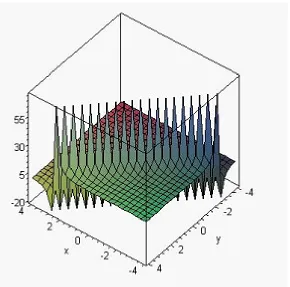
Figure 1. (a) Solitary wave solution corresponding to
(30) fora1= 1, λ0 = 1, σ= 1
Figure 2. (b) Solitary wave solution corresponding to
(30) fora1= 1, λ0 = 1, σ= 1, η0= 1
of nonlinear algebraic equations and by solving it with aid Maple, we obtain
a0= 8λ0V
λ2 0−
3σ
2 +2λ0
3λ20
2 + 3σ
4
, a1=−
12(3σ−2λ20)
r
2λ0V
3σ
2 −λ20
λ2 0−
3σ
2 +2λ0
3λ20
2 + 3σ
4
,
a2=− 48λ0B
λ2 0−
3σ
2 +2λ0
3λ20
2 + 3σ
4
, A=
4λ0V
3σ−2λ2 0
(4.5)
Figure 3. (c) Solitary wave solution corresponding to
(30) fora1=−1, λ0 = 1,σ = 1
ϕ1(η) =− 48λ0B
λ2 0−
3σ
2 +2λ0
3λ20
2 + 3σ
4
×
4λ2
0V2
(3σ−2λ2 0)
2 +
8λ2 0V2
(3σ−2λ2 0)
2tanh
2λ0V
3σ−2λ2 0
(ξ+ξ0)
+ 4λ20V2
(3σ−2λ2 0)
2 tanh
2 2λ0V
3σ−2λ2 0
(ξ−V τ+η0)
−
24λ0V
r
2λ0V
3σ
2 −λ20
λ2 0−
3σ
2+2λ0
3λ20
2 + 3σ
4
h
1 + tanh
2λ0V
3σ−2λ2 0(ξ
−V τ+η0) i
+ 8λ0V
λ2 0−
3σ
2 +2λ0
3λ20
2 + 3σ
4
,
In all figures we suppose ξ=x, τ =y.
5. Conclusions
Figure 4. (d) Solitary wave solution corresponding to
(31) forλ0= 1, σ= 1
variation of electrostatic potential of ion-acoustic solitary waves with different value of the ratio of ion temperature to electron Fermi tem-perature σ is drawn. It has seen that the ion temperature have the significant effect on solitary waves, the width, as well as the amplitude of solitary wave decreases with increasingσ. In summary, we have inves-tigated the nonlinear properties of solitary waves in plasma consisting of degenerate electrons and adiabatic ions. Using the reductive pertur-bation method, the basic set of equations is reduced to KdV equation for lowest order perturbation. Numerical results reveal that compressive solitons has observed. It is essentially important to report in our model of plasma that the amplitude (width) ion-acoustic waves increases as
λ(µ) increases.
References
[2] A. Biswas, Optical Solitons with Time-Dependent Dispersion, Nonlinearity and Attenuation in a Kerr-Law Media, Int. J. Theor. Phys. 48 (2009), 250-260.
[3] A. Biswas, 1-Soliton solution of the K(m,n) equation with generalized evo-lution and time-dependent damping and dispersion,Comput. Math. Appl.
59(8) (2010), 2538-2542.
[4] A. Biswas, M. Fessak, S. Johnson, S. Beatrice, D. Milovic, Z. Jovanoski, Optical soliton perturbation in non-Kerr law media: Traveling wave solu-tion,Optics and Laser Technology44(1) (2012), 263-268.
[5] P. Chatterjee, R. Roychoudhury, Effect of finite ion temperature on ion acoustic solitary waves in a two-temperature electron-plasma system, Canadian Journal of Phys. 75(5)(1997), 337-343.
[6] P. G. Drezin, R. S. Johnson, Solitons, Cambridge University Press, Cam-bridge, 1989
[7] A. E. Dubinov, A. A. Dubinova, Nonlinear theory of ion-acoustic waves in an ideal plasma with degenerate electrons, Phys.-Usp.33(10) (2007), 859-870.
[8] A. Esfandyari-Kalejahi, M. Mehdipoor, M. AkbariMoghanjoughi , Effects of positron density and temperature on ion-acoustic solitary waves in a magnetized electron-positron-ion plasma: Oblique propagation,Physics of Plasmas. 16(5)(2009), 052309.
[9] M. Eslami, M. Mirzazadeh, Topological 1-soliton solution of nonlinear Schrodinger equation with dual-power law nonlinearity in nonlinear op-tical fibers,Eur. Phys. J. Plus 59(8)(2013), 128-140.
[10] N.A. Kudryashov, Simplest equation method to look for exact solutions of nonlinear differential equations, Chaos Soliton Fract. 24 (5)(2005), 12171231.
[11] V. A. Marchenko, M.K. Hudson, Beam-driven acoustic solitary waves in the auroral acceleration region,J. Geophys. Res.100 (1995), 19791.
[12] M. Mirzazadeh, M. Eslami, A. Biswas, Soliton solutions of the general-ized KleinGordon equation by using (GG0)-expansion method,Comp. Appl. Math. 33(2014), 831-839.
[13] Y. Nakamura, J. L. Ferreira and G. O. Ludwig, Experiments on ion-acoustic rarefactive solitons in a multi-component plasma with negative ions,Plasma Phys.33(2) (1985), 237-248.
[14] Y. Nakamura, T. Itoa1 and K. Koga, Excitation and reflection of ion-acoustic waves by a gridded plate and a metal disk, Plasma Phys. 49(2)
(1993), 331-339.
[15] S. Qian, W. Lotko, M.K. Hudson, Dynamics of localized ion-acoustic waves in a magnetized plasma,Phys. Fluids.31(1988), 21902200.
[16] P. K. Shukla, B. Eliasson, Nonlinear aspects of quantum plasma physics, Phys.-Usp.53(1) (2010), 51-76.
[17] T. Stix, Waves in Plasmas. American Institute of Physics, New York, 1992
[18] R. S. Tiwari, Ion-acoustic dressed solitons in electronpositronion plasmas, Physics Letters A.372(19) (2008), 3461-3466.