194
Copyright © 2018. IJEMR. All Rights Reserved.
Volume-8, Issue-1 February 2018
International Journal of Engineering and Management Research
Page Number: 194-200
The Use of Biplot Analysis and Euclidean Distance with Procrustes
Measure for Outliers Detection
Fanny Novika1, Siswadi2 and Toni Bakhtiar3
1Student, Department of Mathematics, Bogor Agricultural University, INDONESIA 2,3Lecturer, Department of Mathematics, Bogor Agricultural University, INDONESIA
1Corresponding Author: [email protected]
ABSTRACT
Outlier is an object that has unique characteristics compared with other objects. Detection of outlier needs to be performed in order to avoid errors in decision-making related to data. Another reason for the detection of outlier is to determine the cause and the meaning of the difference from the outliers. Two methods for detection of outlier are Minimum
Covariance Determinant (MCD) and Fast Minimum
Covariance Determinant (FMCD). Unfortunately, MCD and FMCD require a longer iteration thus it is difficult to detect outlier in large data. In this work, we introduce alternative methods to detect outliers i.e. direct and indirect biplot analyses and direct and indirect Euclidean distances and then we determine the effectiveness of methods in detecting outlier using Procrustes measure. The larger the size of Procrustes measure, the better the method for detecting the outliers. There are six data used in the simulation analysis, i.e. the generated data with the characteristics of one group data, one group data with the outlier, one group data with the top and bottom outliers, two-group data, three-two-group data. Inferred data criteria based on simulation analysis results that MCD, FMCD, indirect biplot and indirect Euclidean distance can’t detect outlier of grouped data. Applicative analysis is the detection of outliers in the welfare data of the Indonesian people based on seven indicators. Papua and DKI Jakarta provinces are concluded as outliers based on all methods. Further analysis reveals that direct Euclidean, indirect Euclidean, and indirect biplot are the best methods. However, direct Euclidean is the simplest method.
Keywords— Biplot Analysis, Euclidean Distance, Fast Minimum Covariance Determinant, Minimum Covariance Determinant, Outlier Detection, Procrustes Measure
I.
INTRODUCTION
Outlier is often found in multivariate analysis, where it describes the behavior of abnormal data, i.e. data
that deviates from the nature of other data [3]. Outlier detection can be used to see the cause and meaning of the difference from the outliers. The existence of an outlier creates errors in interpreting data due to a very large variance of values.
One of the methods which can be used to detect outlier is Minimum Covariance Determinant (MCD) [8]. Determination of homogeneous matrix in MCD leads to a robust MCD method of outlier detection. The homogeneous matrix is derived from some objects of the original data, where the selected objects have the smallest determinant of the covariance matrix compared to other combinations of objects. Nevertheless, the combination of objects from a relatively large number of data using computer will deplete the memory. The relatively large memory requirement for MCD makes this method ineffective. Efforts to overcome this have been done by modifying the MCD method into the Fast Minimum Covariance Determinant (FMCD) [9]. The difference between MCD and FMCD is the weighting of each object at the beginning of the analysis. Another alternative method is needed to detect the evolution more effectively. Biplot analysis [4] and Euclidean distance were used in this study to develop more effective detection outlier methods. The effectiveness of the best method is evaluated by the Procrustes measure [2].
195
Copyright © 2018. IJEMR. All Rights Reserved.
II.
THEORETICAL BASIS
Minimum covariance determinant
Suppose is a matrix data with objects and
variables. Initial step to detect outliers with MCD is choosing objects allocated to homogeneous matrix H
where . The effective is ⌊ ⌋, the value of
is where ⌊ ⌋ denotes the nearest integer less than or equal to [7]. Homogeneous objects can be obtained by determining the combination of objects from that minimize determinant of covariance matrix derived from H. The mean (̅ )and covariance matrix ( )of homogenous matrix are calculated to determine the square of Mahalanobis distance ( ) with
( ) ( ̅ ) ( ̅ )
The outlier is the object that has a square of Mahalanobis distance greater than , where denotes the -quantile of the distribution [7,8].
Fast minimum covariance determinant
The difference between MCD and FMCD is determined by the mean and covariance matrix in Mahalanobis distance. The first step detection outlier with FMCD is determine the mean ̅ and the covariance matrix
of initial matrix data and count a Mahalanobis distance of
i-thobject ( ) where
√( ̅) ( ̅) .
The mean and covariance of Mahalanobis distance with FMCD are defined as
∑
∑
(∑ ( )( ) )
(∑ )
where the weight of each object is determined according
to the following rule: if √ and if
otherwise, so that the Mahalanobis distance with FMCD is
( ) √( ) ( )
[8]. As in MCD, object is categorized as an outlier if ( ) .
Biplot analysis
Biplot is a tool for representing multivariate data in lower-dimensional space (usually two or three) thus, the observation can be represented by one diagram [10]. The main step of biplot analysis is decomposition of initial matrix data to new matrix that has smaller rank. Suppose is matrix data of size that can be factored as with is matrix of size and is matrix of size that has rank [3]. Matrices and are not unique. Suppose is an original data and is corrected matrix data by its mean value, i.e. , where is matrix of size
that all its elements are one. Singular value decomposition of matrix is
with and - ; [5]. When ( , so that
( ) ( ) because . We can conclude:
1. ′ =( 1) , where denotes covariance of
-th and -th variables,
2. √ √ denotes standard
deviation -th variable,
3. correlation of -th variables and -th variables can be explained by
′
4. if rank of matrix is , so
( )′ ( )=( 1)( )′( )
where 𝐒 is covariance matrix of X. Euclidean distance of vector and proportional with Mahalanobis distance of vector and .
When ( ), graphic of biplot objects are those in principal component analysis.
Procrustes measure
Suppose Y is a configuration of points in a dimensional Euclidean space with coordinates given by the following matrix
( )
where is row vector
( )
for and X of size is configuration of points in a dimensional Euclidean space. Configuration Y
needs to be optimally matched X. It is assumed that X and Y
has a same dimension so that . If so ( ) columns of zero are placed at the end of matrix Y so that both configuration are in dimensional space. To measure the difference between two matrix X and Y, Procrustes analysis exploits the sum of the squared distancesE between
X and Y, given by
( ) ∑ ∑( )
( ) ( )
where stands for trace of a matrix [1].
Geometrically, Procrustes measure is minimum distance ( ) that can be determined by series of transformations namely translation, rotation and dilation. In Procrustes analysis, translation is a moving process of all points in a configuration within fixed distance and into the same direction with respect to its centroid. Optimal
translation is and , where
196
Copyright © 2018. IJEMR. All Rights Reserved.
configurations X and Y. The is vector with all elements is one. Rotation is a process of moving all configuration points under the fixed rotation angle without any changes in the points-to-centroid distance. The square of distance after rotation will be minimum by choosing
where is complete form of singular value decomposition from . Dilation on over is
done by multiplying by a scalar , where
that minimized the square of distance between and after dilation. Transformation by translation-rotation-translation gives the minimum possible distance, where the
distance is defined by ( ) (
) ( )[1]. To get the symmetrical Procrustes measure, the normalization is done after translation. Procrustes measure after translation-normalization-rotation-dilation is
( ) ( ) (∑
)
where is a rank matriks X and Y and is singular value
of ̅ ̅ or ̅ ̅ with ̅ and ̅ , where
√ and √ [2].
III.
METHODOLOGY
Data source
The data used in this research are: 1) simulation data which is useful for verifying method with relatively small size data. There are six data used in the simulation analysis, i.e. the generated data with the characteristics of one group data, one group data with the outlier, one group data with the top and bottom outliers, two group data and three group data, 2) applicative data as the application of the detection method of outlier with relatively moderate data size. Data of this research are data of 34 provinces in Indonesia based on indicators of people's welfare according to the Statistics Indonesia 2015 which consists of seven indicators, namely (i) population, (ii) income, (iii) expenditure or consumption per capita, (iv) education, (v) health, (vi) employment and environment and (vii) housing. Each indicator consists of several variables. Before analyzing, data exploration and weighting are done at each variable with standardization.
Data Analysis
Data exploration
Exploration of data is conducted to show the distribution of variable with boxplot. Objects with variables that are significantly different from the mean and the median are potential candidates of outlier. Very different maximum and minimum values show that the range of data in that variable is quite large. Another exploration of data is to see the distribution of data. Data distribution can be seen with
image data in the lower dimension field. Data plot can be provided by biplot analysis.
Outlier detection
The methods that are used to detect the outlier are
a. Minimum Covariance Determinant
Procedures performed in detection of outlier with MCD is supposed is matrix data of size with is the number of objects and is the number of variables. First, ⌊ ⌋ objects of objects are selected by searching for combinations of all possible sets of objects [6]. Selected objects are objects that allocated in a matrix of size having a minimum determinant of covariance matrix. The matrix of the selected objects is named as the homogeneous matrix . The mean of (̅ ) and the inverse of the covariance matrix derived from ( ) are determined. The robust square of Mahalanobis distance of each object is determined ( ̅ ) ( ̅ ), where ( ) is the i-th object. An i-th object ( ) is outlier if ( ̅ ) ( ̅ ) [7].
b. Fast Minimum Covariance Determinant
First step outlier detection with FMCD is input data that size . The mean of each column ( ̅) and the inverse of the covariance matrix ( ) data are determined. The Mahalanobis distance of i-object ( ) is determined.
Each object is weighted with terms if √
and for other. The values and ̅ are changed with and .
The square of Mahalanobis distance of each object is recalculated with and An i-th object ( ) is
outlier if
( - ) - ( - )
[7,8].
c. Biplot analysis
There are two ways to detect the outlier with biplot analysis i.e indirect biplot and direct biplot. Steps for detection of outlier with direct biplot are input data of size and then deviate matrix of data to its mean value calculated by and is an matrix of all elements 1. Then singular value decomposition of matrix calculated by
[4].
197
Copyright © 2018. IJEMR. All Rights Reserved.
is calculated by ( ) where is the first quartile and is the third quartile of distance vector. Objects categorized as outliers are objects that exceed the upper limit.
The step for detection of outlier with indirect biplot is biplot object points is determined, then the distance of each object biplot points with its centroid is also determined. The distance of each object from the closest to the farthest is chosen as much as ⌊ ⌋ objects with the smallest distance. Homogeneous matrix which consists of that is selected from . Euclidean distance from every objects with is determined. Objects categorized as outliers are objects that have a square of distance greater than
.
d. Euclidean distance
There are two ways to detect the outlier with Euclidean distance i.e. indirect Euclidean and direct Euclidean distances. The step for detection of outlier with direct Euclidean distance is input data of size where is
(
)
The mean data is calculated by searching for the mean of each variable as centroid, for the i-th variable the mean of
variable can be determined by ∑ . Each mean of variable is allocated into the mean vector that having one row and column. The Euclidean distance of the k-th object ( ) with centroid data ( ) is calculated by ( )
√∑ ( ) [5]. Euclidean distance of each object is
ordered from the smallest to the largest. The upper limit of the distance vector is given by ( ), where is the first quartile of distance vector and is the third quartile of distance vector. Objects categorized as outliers are those exceeding the upper limit.
The step to detect outlier with indirect Euclidean distance is first input data of size with n is the number of objects and p is the number of variables. The order of distance of each object with its centroid is determined. The homogeneous objects are chosen from ⌊ ⌋ objects which have the smallest distance to centroid. So we get the homogeneous matrix . The Euclidean distance from the i-th object ( ) of the matrix ( ) with centroid of the homogeneous matrix is calculated. The objects categorized as outliers are objects that have a square of distance greater than with p being the number of variables.
Selection of the best method
The best method can be determined by Procrustes measure. The first step is objects categorized as outliers are eliminated equally. For example, with MCD method it is identified two objects that are the outliers then eliminate also
two objects that are identified as outliers by other methods. Procrustes measure of covariance matrix of original data and covariance matrix data without outlier is determined for each method. The best method is that has the largest Procrustes measure.
In some cases it is concluded that the object categorized as outliers are the same objects, so that the best method can’t be identified. Additional steps are needed to find the best method. The best method can be determined by eliminating the farthest object from the centroid next to the outlier. Then the Procrustes measure between covariance matrix of original data with the covariance matrix of data without outliers and the farthest object with the centroid after the outlier is determined. The method with the largest Procrustes measure is the best method.
IV.
RESULTS
Simulation Data
One-group data without outlier
The data in Figure 1 was analyzed by identifying outlier based on direct and indirect biplot, direct and indirect Euclidean distance, MCD and FMCD. The result for the data shows that all objects are not outlier. The result of data analysis is appropriate with the hypothesis. The suggested method can be used to detect outlier from one group data with no outlier candidate.
Figure 1 Plot of one-group data
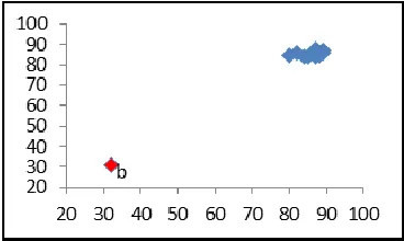
One group data with the outlier
The data in Figure 2 shows that object b is a candidate of outlier. After analyzing with all methods, the result shown that object b is an outlier. So that, the methods can be used in this kind of data.
198
Copyright © 2018. IJEMR. All Rights Reserved.
One group data with the top and bottom outliersThe data in Figure 3 shows that object a is a candidate of top outlier and b is a candidate of bottom outlier. After analyzing with all methods, the result shown that object a and b are outliers. So that, the methods can be used in this kind of data.
Figure 3 Plot of one group data with top and bottom outliers
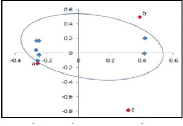
Two-group-data
Two-group data with centered centroid is illustrated in Figure 4. The objects within the ellipse are objects in the homogeneous matrix while the objects outside the ellipse line are the outliers.
Figure 4 Plot two-groups data
This result can’t be trusted because: 1) objects categorized as homogeneous matrices are in fact non-homogeneous objects. This inhomogeneity arises from the generation of a different distribution. 2) a was defined as outlier, but it has a close distance to a group of objects within an ellipse. This is clearly different from the definition of outlier which is the most distinct object of any other objects. Based on this illustration, MCD can’t be used to analyze two group data. So it needs the analysis of depiction of data in a low-dimensional space to avoid objects analysis in groups.
Three-group data
Three-group data is ilustrated in Figure 5. The result is the same as two-group data, i.e. methods can’t be used with this kind of data.
Figure 5 Three-group data
Applicative Data
Exploration of welfare data in Indonesia
The boxplot of the welfare standardized data in Indonesia is illustrated in Figure 6. Based on the figure, the range of each variables are large. The variable X2 (population density) has the smallest interquartile range, but there are some objects that are above the interquartile range. The X12 (partisipation rate of school at age ) has a large interaquartile range. It means that the enrollment rate of the X12 of each province is quite different.
In the welfare data in Indonesia, biplot with two dimensions can be seen in Figure 7. In this case the data spread quite well, there is no data groups. This data can be traced further.
Results data of people's welfare in Indonesia
Provinces categorized as outliers with the largest Procrustes measure are DKI Jakarta and Papua. All methods conclude that Papua and DKI Jakarta are the outliers that has Procrustes measure 0.2968. Procrustes measure of the furthest object with centroid and outlier is calculated to obtain the conclusion the best method to detect the outlier presented in Table 1. In the three farthest objects, the largest Procrustes measure is the direct Euclidean distance, indirect biplot and indirect Euclidean distance. In order to get more accurate conclusion, recalculate the Procrustes measure on the farthest four objects. At four farthest objects, the largest Procrustes measure is the indirect Euclidean distance, direct Euclidean distance and indirect biplot.
199
Copyright © 2018. IJEMR. All Rights Reserved.
V.
CONCLUSION
Outlier detection can be done by direct and indirect biplots and direct and indirect Euclidean distances. As a reference to the detection method with biplot and Euclidean distance, there were also the detection of outliers with MCD and FMCD. Detection with indirect biplot, indirect Euclidean distance, MCD and FMCD require a homogeneous matrix. Homogeneous matrix is a matrix that representing data that is robust to outlier. Determination of homogeneous matrices with biplot and Euclidean distance is considered better than MCD and FMCD in terms of data computing speed with computer. Before processing the data it is highly recommended to check the data properties. The results of checking data properties is the data does not consist of two almost identical groups of objects for all methods using a homogeneous matrix. In provincial data, the outliers are the provinces of DKI Jakarta and Papua. All methods conclude the same thing with Procrustes measure of 0.2968. Further analysis is used to find out the best method with Procrustes measure. Further analysis is done to find out the best method to detect outlier yields direct Euclidean, indirect Euclidean, and indirect biplot are the best methods. Direct Euclidean is the simplest method.
REFERENCES
[1] Bakhtiar T & Siswadi. (2011). Orthogonal procrustes analysis: Its transformation arrangement and minimal distance. International Journal of Applied Mathematics and Statistics, 20(M11), 16-24.
[2] Bakhtiar T & Siswadi. (2015). On the symmetrical property of procrustes measure of distance. International Journal of Pure and Applied Mathematics, 99(3), 315-324. [3] Filzmoser P. 2005. Identification of multivariate outliers: A performance study. Austrian Journal of Statistics, 34(2), 127-138.
[4] Gabriel KR. (1971). The biplot graphic display of matrices with application to principal component analysis.
Biometrika, 58(3), 453-467.
[5] Jolliffe IT. (2002). Principal component analysis. (2nd Edition). New York: Springer-Verlag.
[6] Kaufman L. & Rousseeuw PJ. (2005). Finding group in data an introduction to cluster analysis. New Jersey: John Wiley and Sons.
[7] Lopuhaä HP & Rousseeuw PJ. (1991). Breakdown points of affine equivariant estimators of multivariate location and covariance matrices. The Annals of Statistics, 4, 229-248. [8] Rousseeuw P. (1984). Least median of squares regression.
Journal of the American Statistical Association, 79, 871-880. [9] Rousseeuw PJ & Driessen KV. (1999). A fast algorithm for the minimum covariance determinant estimator.
Technometrics, 41(3), 212-223.
200
Copyright © 2018. IJEMR. All Rights Reserved.
Table 1 Procrustes measure between data without outlier and farthest data from centroid with initial data
Detection method
The number of reduced
objects MCD FMCD
Direct biplot
Indirect biplot
Direct Euclid
Indirect Euclid
Removed provinces
2 Papua Papua Papua Papua Papua Papua
DKI DKI DKI DKI DKI DKI
3 Kalsel Kalsel Jateng NTT NTT NTT
4 Kalteng Kalteng DIY Jateng Jateng Jateng
5 Banten Banten Jatim Jatim Jatim Jatim
Procrustes measure
2 0.2968 0.2968 0.2968 0.2968 0.2968 0.2968
3 0.2994 0.2994 0.2907 0.3403 0.3403 0.3403
4 0.3022 0.3022 0.3054 0.3316 0.3316 0.3316
5 0.2062 0.2062 0.3403 0.3779 0.3779 0.3779
Table 2 Proximity Matrix of outlier and farthest provinces based on Euclidean distance
Provinces Kep.
Riau DKI Jabar Jateng DIY Jatim Banten NTT Kalteng Kalsel Kaltim Papua
Kep. Riau 0
DKI 9.24 0
Jabar 9.50 11.16 0
Jateng 11.61 12.82 5.63 0
DIY 8.66 10.70 9.97 9.80 0
Jatim 11.14 12.35 5.41 1.91 9.35 0
Banten 6.58 9.55 5.41 8.36 8.03 8.22 0
NTT 12.19 14.27 10.78 10.75 10.92 10.88 9.27 0
Kalteng 8.07 10.86 7.95 9.88 8.96 9.73 4.75 8.60 0
Kalsel 8.04 9.87 7.49 8.91 7.86 8.85 4.34 8.64 4.25 0
Kaltim 3.21 8.97 9.05 11.15 8.16 10.67 6.27 11.59 7.55 7.93 0