Learning the Kernel Function via Regularization

Learning the Kernel Function via Regularization

Charles A. Micchelli [email protected]

Department of Mathematics and Statistics State University of New York

The University at Albany 1400 Washington Avenue Albany, NY, 12222, USA

Massimiliano Pontil [email protected]

Department of Computer Science University College London Gower Street, London WC1E, UK

Editor: Peter Bartlett

Abstract

We study the problem of finding an optimal kernel from a prescribed convex set of kernelsK for learning a real-valued function by regularization. We establish for a wide variety of regularization functionals that this leads to a convex optimization problem and, for square loss regularization, we characterize the solution of this problem. We show that, althoughK may be an uncountable set, the optimal kernel is always obtained as a convex combination of at most m+2 basic kernels, where m is the number of data examples. In particular, our results apply to learning the optimal radial kernel or the optimal dot product kernel.

1. Introduction

A widely used approach to estimate a function from empirical data consists in minimizing a regu-larization functional in a Hilbert space

H

of real–valued functions f :

X

→IR, where

X

is a set. Specifically, regularization estimates f as a minimizer of the functional

Q(Ix(f)) +µΩ(f)

where µ is a positive parameter, Ix(f) = (f(xj): j∈INm) is the vector of values of f on the set x=_{xj: j∈INm}and INm={1, . . . ,m}. This functional trades off empirical error, measured by the function Q : IRm_→IR+, with smoothness of the solution, measured by the functionalΩ:

H

→IR+. The empirical error depends upon a finite set_{(xj,yj): j∈INm} ⊂

X

×IR of input-output examples and the function Q depends on y but we suppress it in our notation since it is fixed throughout our discussion. In particular, one often considers the case that Q is defined, for v= (vj: j∈INm)∈IRm, as Q(v) =∑_j∈INmV(vj,yj)where V : IR×IR→IR+is a prescribed loss function.

In this paper we assume that

H

is a reproducing kernel Hilbert space (RKHS)

H

K with kernel K and chooseΩ(f) =_hf,fi, whereh·,_·iis the inner product in

H

K, although some of the ideas we develop may be relevant in other circumstances. This leads us to study the variational problem

Qµ(K):=inf

We recall that an RKHS is a Hilbert space of real-valued functions everywhere defined on

X

such that, for every x_∈

X

, the point evaluation functional defined, for f _∈

H

, by Lx(f):= f(x)is con-tinuous on

H

(Aronszajn, 1950). This implies that

H

admits a reproducing kernel K :

X

×

X

→IR such that, for every x∈

X

, K(x,_·)_∈

H

and f(x) =_hf,K(x,_·)_i. In particular, for x,t∈

X

, K(x,t) =

hK(x,_·),K(t,_·)_iimplying that the m_×m matrix Kx:= (K(xi,xj): i,j∈INm)is symmetric and posi-tive semi-definite for any set of inputs x_⊆

X

.

Often RKHS’s are introduced through the notion of feature map Φ:

X

→

W

, where

W

is a Hilbert space with inner product denoted by(_·,_·). A feature map gives rise to the linear space of all functions f :

X

→IR which are a linear combination of features whose norm is taken to be the norm of its coefficients. That is, for w∈

W

, f = (w,Φ)andhf,fi= (w,w). This space is an RKHS with kernel K defined, for x,t_∈

X

, as K(x,t) = (Φ(x),Φ(t)). Using these equations, the regularization functional in (1) can be rewritten as a functional of w.

Regularization in an RKHS has a number of attractive features, including the availability of effective error bounds and stability analysis relative to perturbations of the data (see, for example, Bousquet and Elisseeff, 2002; Cucker and Smale, 2002; Mukherjee et al., in press; Scovel and Steinwart, 2004; Smale and Zhou, 2003; Vapnik, 1998; Ying and Zhou, 2004; Zhang, 2004; Zhou, 2002). Moreover, one can show that if f is a minimizer of the above functional it has the form

f(x) =

∑

j∈INm

cjK(xj,x), x∈

X

(2)

for some real vector c= (cj: j∈INm)of coefficients (see, for example, De Vito et al., 2005; Girosi, 1998; Kimeldorf and Wahba, 1971; Micchelli and Pontil, 2005; Sch¨olkopf and Smola, 2002; Shawe-Taylor and Cristianini, 2004). This result is known in Machine Learning as the representer theorem. Although it is simple to prove, this result is remarkable as it makes the variational problem (1) amenable for computations.

If Q is convex, the unique minimizer of problem (1) can be found by replacing f by the right hand side of equation (2) in equation (1) and then optimizing with respect to the vector c. For example, when Q is the square error defined for v= (vj: j∈INm)∈IRmas Q(v) =∑j∈INm(vj−yj)

2 the functional in the right hand side of (1) is a quadratic in the vector c and its minimizer is obtained by solving a linear system of equations.

Because of their simplicity and generality, kernels and associated RKHS’s play an increasingly important role in Machine Learning, Pattern Recognition and their applications. This was initiated with the introduction of support vector machines (see, for example, Vapnik, 1998), and continued with the development of many other kernel-based learning algorithms (see, for example, Sch¨olkopf and Smola, 2002; Shawe-Taylor and Cristianini, 2004, and references therein). As kernels can be defined on any input space, kernel-based methods have been successfully applied to learning functions defined on complex data structures, ranging from images, text data, speech data, biological data, among others.

is constructed as linear combinations of features associated to the kernel K, they can provide some guideline for the choice of the kernel. Thus, the choice of the kernel is tied to the problem of choosing a representation of the input. This choice can make a significant difference in practice. For example, techniques such as radial basis functions can perform poorly if the parameter of the radial kernel is not tuned to the given data. A similar circumstance occurs for translation invariant kernels modeled by Gaussian mixtures. When the number of parameters is large cross validation encounters severe computational limitations. To overcome this problem, easily computable approximations to the leave-one-out error have been derived (Chapelle et al., 2002; Wahba, 1990). Nonetheless, these methods are usually non-convex and may lead to undesirable local minima.

In this paper, we propose a method for finding a kernel function which belongs to a compact and convex set

K

. Our method is based on the minimization of the functional in equation (1), that is, we consider the variational problem

inf_{Qµ(K): K∈

K

}. (3)

This problem shares some similarities with recent progress in the context of kernel–based methods (Bach, Lanckriet and Jordan, 2004; Bousquet and Herrmann, 2003; Cristianini et al., 2002; Grae-pel, 2002; Lanckriet et al., 2002, 2004; Lee et al., 2004; Lin and Zhang, 2003; Herbster, 2001; Ong, Smola and Williamson, 2003; Wu, Ying and Zhou, 2004; Zhang, Yeung and Kwok, 2004). In particular, the third and fifth papers motivated our work. In contrast to the point of view of these papers, our setting applies to convex combinations of kernels parameterized by a compact set, a cir-cumstance which is relevant for applications. We also wish to emphasize that although we focus on learning methods based on the minimization of the functional (1), the ideas which we present here may prove useful for learning kernels or feature representations using different forms of regulariza-tion such as entropy regularizaregulariza-tion (Jaakkola, Meila and Jebara, 1999), kernel density estimaregulariza-tion (see, for example, Vapnik, 1998), or one-class SVM (Tax and Duin, 1999) as well as in other Ma-chine Learning frameworks such as those arising in Bayesian learning where a kernel is seen as the covariance of a Gaussian process, (see, for example, Wahba, 1990; Williams and Rasmussen, 1996) or in online learning, (see, for example, Herbster, 2001).

2. Optimal Convex Combination of Kernels

Let

X

be a set. By a kernel we mean a symmetric function K :

X

_×

X

_→IR such that for every finite set of inputs x=_{xj: j∈INm} ⊆

X

and every m∈IN, the m×m matrix Kx:= (K(xi,xj): i,j∈INm) is positive semi-definite. We let

L

(IRm) be the set of m_×m positive semi-definite matrices and

L

+(IRm)the subset of positive definite ones. Also, we use

A

(

X

) for the set of all kernels on the set

X

and

A

+(

X

)for the subset of kernels K such that, for each input x, Kx∈

L

+(IRm). We also occasionally refer to the set of all symmetric m_×m matrices and use

S

(IRm)to denote them.

According to Aronszajn and Moore (see Aronszajn, 1950), every kernel has associated to it an (essentially) unique Hilbert space

H

K with inner producth·,·isuch that K is its reproducing kernel. This means that for every f _∈

H

Kand x∈

X

,hf,Kxi= f(x), where Kx is the function K(x,·).

Let D :=_{(xj,yj): j∈INm} ⊂

X

×IR be prescribed data and y the vector (yj : j∈INm). For each f _∈

H

K, we introduce the information operator Ix(f):= (f(xj): j∈INm) of values of f on the set x :=_{xj: j∈INm}. We prescribe a nonnegative function Q : IRm→IR+ and introduce the

regularization functional

Qµ(f,K):=Q(Ix(f)) +µkfk2K (4) where_kf_k2_K :=_hf,f_i, µ is a positive constant and Q depends on y but we suppress it in our no-tation as it is fixed throughout our discussion. A noteworthy special case of Qµ is the square loss regularization functional given by

Sµ(f,K):=ky−Ix(f)k2+µkfk2K (5) where_{k · k}is the standard Euclidean norm on IRm. There are many other choices of the functional Qµwhich are important for applications, see the work of Vapnik (1998) for a discussion.

Associated with the functional Qµand the kernel K is the variational problem

Qµ(K):=inf{Qµ(f,K): f ∈

H

K} (6)

which defines a function Qµ:

A

(

X

)→IR+. We remark, in passing, that all of what we say about problem (6) applies to functions Q which are bounded from below on IRmas we can merely adjust the expression (4) by a constant independent of f and K. Let us first point out that the infimum in (6) is achieved, at least when Q is continuous.

Lemma 1 If Q : IRm_→IR+ is continuous and µ is a positive number then the infimum in (6) is

achieved for a function in

H

K. Moreover, when Q is convex this function is unique.

PROOF. The proof of this fact is straightforward and uses weak compactness of the unit ball in

H

K. The uniqueness of the solution relies on the fact that when Q is convex Qµ is strictly convex

because µ is positive.

The point of view of this paper is that the functional (6) can be used as a design criterion to select the kernel K. To this end, we specify an arbitrary convex subset

K

of

A

(

X

)and focus on the problem

Qµ(

K

) =inf{Qµ(K): K∈

K

}. (7)

Recall that the solution of (6) is given in the form f =∑_j∈INmcjKxj for some vector c := (cj: j∈

representation for learning the function f is central for many diverse applications of kernel-based algorithms in Machine Learning. Moreover, the coefficient vector c is found as the solution of the finite dimensional variational problem

Qµ(K):=min{Q(Kxc) +µ(c,Kxc): c∈IRm}

where(_·,_·)is the standard inner product on IRm.

Before we address basic questions concerning the variational problem (7) we describe some terminology that allows for a precise description of our observations. Every input set x and set of basic kernels

G

on

X

×

X

determines a set of matrices in

L

(IRm), namely

G

(x):=_{Gx: G∈

G

}.

Obviously, it is the set of matrices

K

(x)that affects the variational problem (7). Note that

G

(x)

being a subset of

S

(IRm)is identifiable as a set of vectors in IRN, where N :=m(m₂+1). As such

G

(x)

inherits the standard topology from IRN. That is, convergence of a sequence of matrices in

G

(x)

means that the respective elements of the matrices converge. For this reason, we use

G

(the closure of

G

) to mean the set of all kernels K on

X

×

X

with the property that for each x_⊆

X

, the matrix Kx∈

G

(x), the closure of

G

(x)relative to IRN. We say a set of kernels

G

is closed provided that

G

=

G

. Also, we say

G

is a compact convex set of kernels whenever for each x_⊆

X

,

G

(x) is a compact convex set of matrices in

S

(IRm). Our next result establishes the existence of the solution to problem (7).

Lemma 2 If

K

is a compact and convex subset of

A

+(

X

)and Q : IRm→IR is continuous then the

minimum of (7) exists.

PROOF. Fix x_⊆

X

, choose a minimizing sequence of kernels_{Kn: n_∈IN_}, that is, limn→∞Qµ(Kn) = Qµ(

K

)and a sequence of vectors{cn: n∈IN}such that

Qµ(Kn) =Q(Kxncn) +µ(cn,Kxncn).

Since

K

is compact there is a subsequence_{Kn(`):`_∈IN_}such that lim`→∞Kxn(`)=K˜x, for some

kernel ˜K∈

K

. We claim that{cn: n∈IN}is bounded. Indeed, there is a positive constantρsuch that(cn,K_xncn)_≤ρ. Set an= _kc_cnn_k so that(an,K_xnan)≤ _kcρn_k2 and choose a convergent subsequence

{an(`(q))_{: q∈IN}such that lim}

q→∞an(`(q))=a andkak=1 for some vector a∈IRm. If the sequence

{cn: n_∈IN_}is not bounded we conclude that(a,K˜xa) =0 contradicting our hypothesis that ˜K∈

A

+(

X

). Hence there is a subsequence{cn(`(q)): q∈IN}such that limq→∞cn(`(q))=c, for some c∈IRm. Therefore, we conclude that

Qµ(

K

) =Q(K˜xc) +µ(c,K˜xc)≥Qµ(K˜)

from which it follows that Qµ(

K

) =Qµ(K˜).

The proof of this lemma requires that all kernels in

K

are in

A

+(

X

). If we wish to use kernels K only in

A

(

X

) we may always modify them by adding any positive multiple of the delta function kernel∆defined, for x,t_∈

X

, as

∆(x,t) =

1, x=t

that is, replace K by K+a∆where a is a positive constant.

There are two useful cases of a set

K

of kernels which are compact and convex. The first is formed by the convex hull of a finite number of kernels in

A

+(

X

). The second example extends this to a compact Hausdorff spaceΩ, (see, for example, Royden, 1988), and a mapping G :Ω_→

A

+(

X

). For eachω_∈Ω, the value of the kernel G(ω)at x,t_∈

X

is denoted by G(ω)(x,t)and we assume that the function ofω7→G(ω)(x,t)is continuous onΩfor each x,t∈

X

. When this is the case we say G is continuous. We let

M

(Ω)be the set of all probability measures onΩand observe that

K

(G):=

Z

ΩG(ω)d p(ω): p∈

M

(Ω)

(9)

is a compact and convex set of kernels in

A

+(

X

). The compactness of the set

K

(G)is a consequence of weak∗-compactness of the unit ball of the dual space of C(Ω), the set of all continuous real-valued functions g onΩwith norm_kg_kΩ:=max_{|g(ω)_|:ω_∈Ω_}(Royden, 1988). For example, we chooseΩ= [a,b], where a>0 and G(ω)(x,t) =e−ωkx−tk2, x,t_∈IRd,ω_∈Ω, to obtain radial kernels, or G(ω)(x,t) =eω(x,t), x,t_∈IRdto obtain dot product kernels. Note that the choiceΩ=INn corresponds to our first example.

In preparation for the next theorem we need to express the set

K

(G)in an alternate form. We have in mind the following basic fact.

Lemma 3 IfΩis a compact Hausdorff space, G :Ω→

A

+(

X

)a continuous map as defined above

and

G

:=_{G(ω):ω_∈Ω_}then

K

(G) =co

G

.

PROOF. First, we shall show that coG _⊆

K

(

G

). To this end, we let K_∈co

G

and x_⊆

X

. By the definition of convex hull, we obtain, for some sequence of probability measures_{p`:`∈IN},

that Kx=lim`→∞R<sub>Ω</sub>Gx(ω)d p`(ω)where each p`is a finite sum of point measures. Since for each

`_∈IN,R

ΩGx(ω)d p`(ω)∈

K

(G) and

K

(

G

)is closed it follows that Kx⊆

K

(G), that is, we have

established that coG ⊆

K

(

G

).

On the other hand, if there is a kernel K _∈

K

(G) which does not belong to coG then there is an input set x such that Kx∈/ co

G

(x) while Kx =

R

ΩGx(ω)d p(ω) for some p∈

M

(Ω). Hence,

there exists a hyperplane which separates the matrix Kxfrom the set of matrices coG(x)(Royden,

1988). This means that there is a linear functional L on

S

(IRm)and c_∈IR such that L(Kx)>c but

L(Gx(ω))<c for allω∈Ω. We integrate the last inequality overω∈Ωrelative to the measure d p

and conclude by the linearity of L that L(Kx)<c, a contradiction. This concludes the proof.

Observe that the set

G

=_{G(ω):ω_∈Ω_}in the above lemma is compact since G is continuous andΩcompact. In general, we wish to point out a useful fact about the kernels in coG whenever

G

is a compact set of kernels. To this end, we recall a theorem of Caratheodory (see, for example, Rockafellar, 1970, Ch. 17).

Theorem 4 If A is a subset of IRn then every a_∈coA is a convex combination of at most n+1 elements of A.

An immediate consequence of the above theorem is the following fact which we shall use later.

In particular, we have the following corollary.

Corollary 6 If

G

is a compact set of kernels on

X

×

X

then co

G

is a compact set of kernels. Moreover, for each input set x a matrix C_∈co

G

(x)if and only if there exists a kernel T which is a convex combination of at most m(m₂+1)+1 kernels in

G

and Tx=C.

Our next result shows whenever

K

is the closed convex hull of a compact set of kernels

G

that the optimal kernel lies in a the convex hull of some finite subset of

G

.

Theorem 7 If

G

⊆

A

+(

X

)is a compact set of basic kernels,

K

=co

G

, Q : IRm→IR+is continuous

and µ is a positive number then there exists

T

⊆

G

containing at most m+2 basic kernels such that Qµadmit a minimizer ˜K∈co

T

and Qµ(

T

) =Qµ(

K

).

PROOF. Let(cˆ,_Kˆ_)∈IRm_×

_K

_{be a minimizer of Q}

µ, that is, we have that

Qµ(

K

) =min{Q(Kˆxc) +µ(c,Kˆxc): c∈IRm}=Q(Kˆxcˆ) +µ(cˆ,Kˆxcˆ).

We define the set of vectors

U

:=_{(Kxcˆ,(cˆ,Kxcˆ)): K∈

K

} ⊂IRm+1. Note that

U

=co

V

where

V

=_{(Gxcˆ,(cˆ,Gxcˆ)): G∈

G

}and

V

is compact since

G

is compact. By Lemma 5 the vector

(_Kˆ_{xcˆ,(cˆ,Kxcˆ))can be written as a convex combination of at most m+2 vectors in}

_V

_{, that is}

(_Kˆ_xcˆ,(cˆ,Kˆ_{xcˆ)) = (K}˜_xcˆ,(cˆ,K˜_xcˆ))

where ˜K is the convex combination of at most m+2 kernels in

G

. Consequently, we have that

Qµ(

K

) = Q(K˜xcˆ) +µ(cˆ,K˜x,cˆ)

≥ min_{Q(_K˜_{xc) +µ(c,K}˜_{xc): c∈IR}m

}

= Qµ(K˜)≥Qµ(

K

)

implying that Qµ(Kˆ) =Qµ(K˜).

Note that Theorem 7 asserts the existence of a q which is at most m+2, that is, an optimal kernel is expressed by a convex combination of at most m+2 kernels.

Note that in the definition of Qµ(

K

)we minimize first over f∈

H

Kand then over K∈

K

. There arises the question of what would happen if we interchange these minima. We address this issue in the case that

K

is the convex hull of a finite set of kernels. To this end, we use the notation L

j∈INn

H

Kj for the direct sum of the Hilbert spaces{

H

Kj : j∈INn}.

Lemma 8 If

K

n={Kj: j∈INn}is a family of kernels on

X

×

X

and f ∈Lj∈INn

H

Kj then

inf_{kf_kK : K∈co

K

n}=min

(

∑

j∈INn

kfjkKj: f =

∑

j∈INn

fj, f`∈

H

K`, `∈INn

)

As the result is not needed in our subsequent analysis we postpone its proof to the appendix (for related results, see also, Herbster, 2004; Lin and Zhang, 2003). We note that the expression on the right hand side of equation (10) is an intermediate norm forL

j∈INn

H

Kj (see Bennett and Sharpley,

1988, p. 97) for a discussion. This lemma suggests a reformulation of our extremal problem (7) for kernels of the form (9) where G is expressed in terms of a feature map. Although this fact is interesting, it is not central to our point of view in this paper and, so, we describe it in the appendix. Next, we establish that the variational problem (7) is a convex optimization problem. Specif-ically, we shall show that if the function mapping Q : IRm_→ IR is convex then the functional Qµ:

A

+(

K

)→IR+ is a convex as well. It is curious that this does not seem to follow directly from the definition of Qµ. We take a sojourn through the notion of conjugate function. Recall that the conjugate function of Q denoted by Q∗: IRm_→IR is defined, for every v_∈IRm, as

Q∗(v) =sup_{(c,v)₋Q(c): c_∈IRm_}

and it follows, for every c_∈IRm_{, that}

Q(c) =sup_{(c,v)₋Q∗(v): v_∈IRm_}

(see, for example, Rockafellar, 1970; Borwein and Lewis, 2000). A nice recent application of the conjugate function to linear statistical models appears in (Zhang, 2002).

The proof we present below for the convexity of Qµ :

A

+(

X

)→IR+ is based upon the von Neumann minimax theorem which we record in the appendix. We begin by introducing for each r>0 a functionφr: IR+→IR+ defined, for t∈IR+, as

φr(t):=µ( 1 2µ

√

t₋r)2₊₋ 1

4µt

where(z)+:=max(0,z). Note that

lim

r→∞φr(t) =− 1 4µt

pointwise for t>0. Also, for each fixed t>0,φr(t)is a non-increasing function of r and, for each r>0,φris continuously differentiable, decreasing and convex on IR+.

Lemma 9 If K_∈

A

(

X

), x a set of m distinct points of

X

such that Kx∈

L

+(IRm)and Q : IRm→IR

a convex function, then there exists r0>0 such that for all r>r0there holds the formula

Qµ(K) =sup{φr((v,Kxv))−Q∗(v): v∈IRm}. (11)

PROOF. By the definition of Qµwe have that

Qµ(K) =min{sup{(Kxc,v)−Q∗(v) +µ(c,Kxc): v∈IRm}: c∈IRm}.

According to Lemma 2 the minimum above exists. Therefore, there is a r0>0 such that for all r>r0we have that

By the minimax theorem, see Theorem 22 in the appendix, we conclude that

Qµ(K) =sup{min{(Kxc,v)−Q∗(v) +µ(c,Kxc): c∈IRm,(c,Kxc)≤r2}: v∈IRm}.

For each v_∈IRm, we shall now explicitly compute the minimum of the above expression. To this end, we let Kx:=B2where B is a m×m positive definite matrix, that is, B is the square root of Kx,

and observe that

min_{(c,Kxv) +µ(c,Kxc):(c,Kxc)≤r2}=min{µkBc+

1 2µBvk

2

−_4µ1 kBv_k2:_kBc_{k ≤}r_}.

If the vector c0:=−_2µ1v has the property thatkBc0k ≤r, that is, kBvk ≤2µr then the minimum above is_−4µ1_kBv_k2, otherwise_kBv_k>2µr and the triangle inequality says that

kBc+ 1

2µBvk ≥ 1

2µkBvk − kBck ≥ 1

2µkBvk −r.

Since, for the vector ˆc :=₋ vr

kBvk, we have that

kB ˆc+ 1

2µBvk= 1

2µkBvk −r

this inequality is sharp. Therefore, we get that

Qµ(K) =sup

µ( 1

2µkBvk −r) 2 +−

1 4µkBvk

2

−Q∗(v): v_∈IRm

and the result follows by the definition ofφr.

Let us specialize this lemma to the example of the square loss S defined, for w_∈IRm, as S(w) =

ky₋w_k2. In this case, the conjugate function is given explicitly for v_∈IRmas S∗(v) =max_{(w,v)_{− k}w₋y_k2: w_∈IRm_}=1

4kvk

2_{+ (y,v).}

We shall show later in Lemma 14 by a direct computation without the use of the conjugate function that Sµ=µ(y,(Kx+µI)−1y). Alternatively, if we formally let r=∞in the right hand side of equation

(11) we get

sup

−_4µ1 (v,(Kx+µI)v)−(y,v): v∈IRm

which by a direct computation equals µ(y,(Kx+µI)−1y). This suggests that Lemma 9 may even

hold when r=∞and without the hypothesis that Kx∈

L

+(IRm). We shall confirm this with another version of the von Neumann minimax theorem.

Lemma 10 If K_∈

A

(

X

), x a set of m distinct points of

X

such that Kx∈

L

+(IRm)and Q : IRm→IR

a convex function, then there holds the formula

Qµ(K) =sup

−1

4µ(v,Kxv)−Q

∗_{(v): v∈IR}m

PROOF. Theorem 23 applies since Kx ∈

L

+(IRm). Indeed, we let f(c,v) = (Kxc,v)−Q∗(v) + µ(c,Kxc),

A

=

B

=IRmand v0=0 then the set{c : c∈IRm,f(c,v0)≤λ}is compact and all the hypotheses of Theorem 23 hold. Hence, we may proceed as in the proof of Lemma 9 with r=∞. To interpret Lemma 9, we say that AB whenever A,B_∈

L

(IRm), if B₋A is positive semi-definite. We also say, for K,J_∈

A

(

X

), that KJ if KxJxfor every x⊆

X

.

Definition 11 A functionφ:

B

_→IR is said non–decreasing on

B

_⊆

A

(

X

)if, for every A,B_∈

B

with AB it follows thatφ(A)_≤φ(B). If the reverse inequality holds we sayφis non–increasing.

Definition 12 A functionφ:

B

→IR is said convex on

B

⊆

A

(

X

)if, for every A,B_∈

B

andλ_∈[0,1]

there holds the inequality

φ(λA+ (1₋λ)B)_≤λφ(A) + (1₋λ)φ(B). (12)

If the reverse of inequality (12) holds we say that theφis concave.

Proposition 13 If Q : IRm_→IR+ is convex then for every µ>0 the function Qµ:

A

+(

X

)→IR+is

convex and non-increasing.

PROOF. The proof of the proposition follows from Lemma 9. Specifically, equation (11) expresses

Qµas the supremum of a family of functions which are convex and non-increasing on

A

(

X

). We note that the convexity of the function Qµ was already proven by Lanckriet et al. (2004) for the hinge loss and stated in (Ong, Smola and Williamson, 2003) for differentiable convex loss functions.

3. Square Regularization

In this section we exclusively study the case of the square loss regularization functional Sµin equa-tion (5) and provide improvements and simplificaequa-tions of our previous results. We begin by deter-mining the explicit expression for this functional which we briefly mentioned earlier after the proof of Lemma 9.

Lemma 14 For any kernel K, inputs x :=_{xj: j∈INm}, samples y= (yj: j∈INm) and positive constant µ we have that

Sµ(K) =µ(y,(µI+Kx)−1y) (13)

where I is the m_×m identity matrix.

PROOF. We have that Sµ(K) =min{R(c): c∈IRm}where for each c∈IRmwe set R(c):=ky− Kxck2+µ(c,Kxc). We define the vector w := (µI+Kx)−1y, observe that R(w) = (y,µ(µI+Kx)−1y)

and for every vector c_∈IRmwe have that

R(c) =R(w) +_kKx(w−c)k2+µ(c−w,Kx(c−w)).

From this lemma we conclude, when the matrix Kxis in

L

+(IRm)then limµ→0µ−1Sµ(K) =γ(Kx),

where for every A_∈

L

+(IRm) we setγ(A):= (y,A−1y). The functionγ:

L

+(IRm)→IR+ has the alternate form

1

γ(A) :=min{(c,Ac): c∈IR

m_{,(c,y) =1}

}, A_∈

L

+(IRm) (14)

and the unique vector which achieves this minimum is given by

c(A):= A−

1_y

(y,A−1_y). (15)

A proof of these facts follow directly from the Cauchy-Schwarz inequality for the inner product

(u,Av), u,v_∈IRm. Moreover, this alternate form forγ(A) connects the functionγto the minimal norm interpolant in

H

Kto the data D. Let us explain this connection next.

Recall, for every kernel K on

X

×

X

, that the minimal norm interpolation to the data D is the solution to the variational problem

ρ(K):=min_{kf_k2_K: f _∈

H

K,f(xj) =yj,j∈INm}. (16) The following result is well-known (for a proof see, for example, Micchelli and Pontil, 2005).

Proposition 15 If K_∈

A

(

X

)and x is an input set in

X

such that the matrix Kxis in

L

+(IRm)then

the solution of the minimal norm interpolation problem (16) is unique and is given by

f =

∑

j∈INm

cjK(xj,·)

where the coefficient vector c= (cj: j∈INm)solves the linear system of equations Kxc=y and we

have that

ρ(K) =γ(Kx) = (y,Kx−1y). (17)

The functionγ:

L

+(IRm)→IR+is continuous. We record additional facts about this function in the next two lemmas.

Lemma 16 The functionγis non–increasing and whenever A,B_∈

L

+(IRm),γ(A) =γ(B)if and only

if A−1y=B−1y.

PROOF. If AB then for every c∈IRm,(c,Ac)≤(c,Bc)and it follows that _γ(1_A) ≤_γ(1_B). Clearly

A−1y=B−1y implies thatγ(A) =γ(B). On the other hand ifγ(A) =γ(B), the inequalities _γ(1_A)≤

(c(B),Ac(B))_≤(c(B),Bc(B)) = _γ(1_B)imply that c(A) =c(B)and the result follows.

Lemma 17 The function γis convex and the function γ−1 concave. Moreover, for every A,B_∈

L

+(IRm),λ∈[0,1], we have that

1

γ(λA+ (1₋λ)B) =λ

1

γ(A)+ (1−λ)

1

γ(B) (18)

PROOF. For everyλ∈[0,1]we define the matrix D_λ=λA+ (1−λ)B and for all c∈IRmfor which

(c,y) =1 note that

(c,D_λc) =λ(c,Ac) + (1₋λ)(c,Bc)_≥λ 1

γ(A)+ (1−λ)

1

γ(B). (19)

Consequently, we have that _γ(D1 λ)≥λ

1

γ(A)+ (1−λ)γ(1B), showing thatγ−1is concave. Alternatively, equation (14) expresses γ−1(A) as the minimum of a family of functions which are linear in the matrix A and henceγ−1is concave. Similarly, using this equation we have that

γ(A) =max(c,Ac)−1: c_∈IRm,(c,y) =1 thereby expressingγas a maximum of a family of convex functions.

If (18) holds, we choose c=c_λ:=c(D_λ)in (19) and conclude by the uniqueness of the vector c(A)in equation (15) that c_λ=c(A) =c(B). Conversely, when this conclusion holds we have that

1

γ(D_λ) = λ(cλ,Acλ) + (1−λ)(cλ,Bcλ)

= λ(c(A),Ac(A)) + (1₋λ)(c(B),Bc(B))

= λ 1

γ(A)+ (1−λ)

1

γ(B)

which concludes the proof.

Lemma 16 and 17 established that the functionφ:

L

+(IRm)→IR defined, for some d∈IRmand all A_∈

L

+(IRm), asφ(A) = (d,A−1d)is non-increasing and convex (see also the work of Marshall and Olkin, 1979).

Proposition 15 and Lemma 14 connects minimal norm interpolation to square loss regulariza-tion. This connection allows us in this section to turn our attention to the functionρ:

A

(

X

)_→IR+ and consider the variational problem

ρ(

K

):=inf_{ρ(K): K_∈

K

} (20)

where

K

is a prescribed set of kernels. The approach of Lemma 2 applies directly to establish the following lemma.

Lemma 18 If

K

is a compact and convex set of kernels in

A

+(

X

)then the minimum of (20) exists. Our next result describes the solution of the problem of determining ρ(

K

) for the case that

K

=co

K

nwhere

K

n={K`:`∈INn}is a prescribed finite subset of

A

+(

X

). In its presentation we use the notion Kx,` for the matrix(K`)x.

Theorem 19 If

K

n={Kj: j∈INn} ⊂

A

+(

X

)there exists a kernel ˆK=∑j∈JλjKj∈co

K

n, where J_⊆INn, card(J)≤min(m+1,n)with∑j_∈Jλj=1 such that, for every j∈J,λj>0,

(cˆ,Kx,jcˆ) =max{(cˆ,Kx,`cˆ):`∈INn}, cˆ=c(Kˆx),

ρ(

K

) =ρ(_Kˆ_{) = (y,K}ˆ−1

and for every c∈IRmwith(c,y) =1 and every K∈co

K

n

(cˆ,Kxcˆ)≤(cˆ,Kˆxcˆ)≤(c,Kˆxc). (21)

Inequality (21) expresses the fact that the pair(cˆ,_Kˆ_{)is a saddle point for the minimax problem}

˜

ρ−1_=min

{max_{(c,Kxc): K∈co

K

n}: c∈IRm,(c,y) =1}.

The existence of(cˆ,_Kˆ_{)above implies that the minimum and maximum can be interchanged, that is,}

max_{min_{(c,Kxc): c∈IRm,(c,y) =1}: K∈co

K

n} (22)

= min_{max_{(c,Kxc): K∈co

K

n}: c∈IRm,(c,y) =1}. (23)

Moreover, any ˆc and ˆK with the properties described in Theorem 19 is a saddle point of this minimax problem. Indeed, the upper bound in (21) follows from the definition of the vector ˆc and the function

γdefined earlier, see equations (14) and (15). The lower bound follows from the fact that for any K_∈co

K

nwe have that(cˆ,Kxcˆ)≤max{(cˆ,Kx,`cˆ):`∈INn}.

Let us now turn to the existence of ˆK. Note that by equation (14) and Proposition 15 the expres-sion in (22) is 1/ρ(

K

), the reciprocal of the quantity of interest to us. It is the quantity in equation (23) which we examine in the proof of Theorem 19 and it has been denoted by ˜ρ−1_{. A consequence} of Theorem 19 is that ˜ρ=ρ(

K

). Certainly, by their definitions it is clear that ˜ρ_≤ρ(

K

).

We now present the proof of Theorem 19.

PROOF. Let ˜c be a solution to problem (23). We define the set

J∗_≡J(c˜):=

j : j_∈INn,(c˜,Kx,jc˜) =max{(c˜,Kx,ic˜): i∈INn}

the convex functionϕ: IRm_→IR by setting for each c_∈IRm,ϕ(c):=max_{(c,Kx,jc): j∈INn}and note that by Lemma 24 the directional derivative ofϕ along the “direction” d_∈IRm, denoted by

ϕ0

+(c; d), is given by

ϕ0

+(c; d) =2 max{(d,Kx,jc): j∈J(c)}. Since ˜c is a minimum for (14) we have that

max_{(d,Kx,jc˜): j∈J∗} ≥0

for every d_∈IRmsuch that(d,y) =0. Let

M

be the convex hull of the set of vectors

N

:=_{Kx,jc :˜ j_∈J∗_{} ⊂}IRm. Since

M

⊆IRm, by the Caratheodory theorem (see, for example, Rockafellar, 1970, Ch. 17) every vector in

M

can be expressed as a convex combination of at most q :=min(m+

1,_|J∗_|)_≤min(m+1,n)elements of

N

. We will show that

M

intersects the line spanned by the vector y. Indeed, if these two sets did not intersect then there exists a hyperplane_{c : c_∈IRm,(w,c)+

α=0_}, whereα_∈IR,w_∈IRm, which strictly separates them, that is,

(w,ty) +α>0, t_∈IR

and

(see, for example, Royden, 1988).

The first condition, for t=0, implies thatα>0 and since t can take any real value we also have that(w,y) =0. Consequently, from equation (24) we get that

max_{(w,Kx,jc˜): j∈J∗}<0

which contradicts our hypothesis that ˜c is a minimum. Thus, it must be the case that t0y∈

M

for some t0_∈IR, that is,

t0y=

∑

j∈J

γjKx,jc˜ (25)

for some subset J of J∗of cardinality at most q and positive constantsγj with∑j∈Jγj =1. Taking the inner product of both sides of equation (25) with ˜c, and recalling the fact that (c˜,y) =1 we obtain that t0=ρ˜−1_{. Setting}

ˆ K :=

∑

j∈J

γjKj

we have from (25) that ˜c=ρ˜−1_Kˆ−1

x y, and ˜ρ= (y,Kˆx−1y). Therefore, by Proposition 15 we conclude

that ˜ρ=ρ(_Kˆ_{)and ˜c=c where ˆˆ c is defined in the theorem. In particular, we obtain ˜ρ≥ρ(}

_K

_{)and so} by our previous remarks just before the beginning of the proof, we conclude that ˜ρ=ρ(

K

). Recall, that earlier we introduced the class

K

(G) induced by a continuous mapping G :Ω_→

A

+(

X

)whereΩis a compact Hausdorff space. Theorem 15 extends to this generality. No essential difference occur in the proof. However, the conclusion is striking. Not only do we characterize the optimal kernel ˆK_∈

K

(G)but we show that it comes from a discrete probability measure ˆp_∈

M

(Ω)

with at most m+1 atoms, that is, ˆK=R

ΩG(ω)d ˆp(ω).

Theorem 20 IfΩis a compact Hausdorff topological space and G :Ω_→

A

+(

X

)is continuous then

there exists a kernel ˆK=R

ΩG(ω)d ˆp(ω)∈

K

(G) such that ˆp is a discrete probability measure in

M

(Ω)with at most m+1 atoms. Moreover, for any atom ˆω_∈Ωof ˆp, we have that

(cˆ,Gx(ωˆ)cˆ) =max{(cˆ,Gx(ω)cˆ):ω∈Ω}, cˆ=c(Kˆx),

ρ(

K

) =ρ(_Kˆ_{) = (y,K}ˆ−1

x y)

and for every c_∈IRmwith(c,y) =1 and every K_∈

K

(G)

(cˆ,Kxcˆ)≤(cˆ,Kˆxcˆ)≤(c,Kˆxc).

PROOF. Let ˜c be a solution to problem (23) where co

K

nis replaced by

K

(G)and define the set

Ω∗_{≡Ω(c˜):={τ:τ∈Ω,(c˜,G}

x(τ)c˜) =max{(c˜,Gx(ω)c˜):ω∈Ω}}.

where we denoted the matrix (G(ω))x by Gx(ω). We define the convex function ϕ: IRm→ IR

by setting for each c_∈IRm_, ϕ_{(c):=max{(c,G}

x(ω)c):ω∈Ω} and note that by Lemma 24 the

directional derivative ofϕalong the “direction” d_∈IRm, denoted byϕ0₊(c; d), is given by

ϕ0

+(c; d) =2 max{(d,Gx(ω)c):ω∈Ω∗}.

Since ˜c is a minimum for (14) we have that

for every d∈IRmsuch that(d,y) =0. Let

M

be the convex hull of the set of vectors

N

:=_{Gx(ω)c :˜ ω∈Ω∗} ⊂IRm. Since

M

_⊆IRm, by the Caratheodory theorem every vector in

M

can be expressed as a convex combination of at most m+1 elements of

N

. We will show that

M

intersects the line spanned by the vector y. Indeed, if these two sets did not intersect then there exist a hyperplane

(w,c) +α=0,α_∈IR,w_∈IRm, which strictly separates them, that is,

(w,ty) +α>0, t_∈IR

and

(w,Gx(ω)c˜) +α<0, ω∈Ω∗, (26)

(see Royden, 1988).

The first condition, for t=0, implies thatα>0 and since t can take any real value we also have that(w,y) =0. Consequently, from equation (26) we get that

max_{(w,Gx(ω)c˜):ω∈Ω∗}<0.

which contradicts our hypothesis that ˜c is a minimum. Thus, it must be the case that t0y∈

M

for some t0_∈IR, that is,

t0y= Z

ΩGx(ω)cd ˆ˜ p(ω) (27)

where ˆp_∈

M

(Ω) is a discrete probability measure with at most m+1 atoms. Taking the inner product of both sides of equation (27) with ˜c, and recalling the fact that(c˜,y) =1 we obtain that t0=ρ˜−1. Setting

ˆ K :=

Z

ΩGx(ω)d ˆp(ω)

we have from (27) that ˜c=ρ˜−1_Kˆ−1_{y, and ˜ρ= (y,Kˆ}−1_{y). Therefore, by Proposition 15 we conclude} that ˜ρ=ρ(_Kˆ_{)and ˜c=c where ˆˆ c is defined in the theorem. In particular, we obtain ˜ρ≥ρ(}

_K

_)and so by our previous remarks we conclude that ˜ρ0=ρ(

K

).

This theorem applies to the Gaussian kernel.

Corollary 21 If a>0 and N :[a,b]_→

A

+(

X

)is defined as

N(ω)(x,t) =e−ωkx−tk2, x,t_∈IRd,ω_∈IR+

then there exists a kernel ˆK=R

ΩN(ω)d ˆp(ω)∈

K

(N)such that ˆp is a discrete probability measure

in

M

(Ω)with at most m+1 atoms. Moreover, for any atom ˆω_∈Ωof ˆp, we have that

(cˆ,Nx(ωˆ)cˆ) =max{(cˆ,Nx(ω)cˆ):ω∈Ω}, cˆ=c(Kˆx),

ρ(

K

(N)) =ρ(_Kˆ_{) = (y,K}ˆ−1

x y)

and for every c_∈IRmand K_∈

K

(N)we have that

We note that, in view of equations (13) and (17), Theorem 19 and Theorem 20 apply directly, up to an unimportant constant µ, to the square loss functional by merely adding the kernel µ∆to the class of kernels considered in these theorems. That is, we minimize the quantity in equation (17) over the compact convex set of kernels

˜

K

=_{{K : ˜}˜ _{K=K+µ∆, K∈}

_K

_}

where the kernel∆is defined in equation (8).

An important example of the above construction is to choose Kj to be polynomials on IRd, namely Kj(x,t) = (x,t)j, x,t∈IRd. From a practical point of view we should limit the range of the index j and therefore Theorem 19 adequately covers this case. On the contrary if we decide to use, as it is done often, Gaussians, there arises not only how many Gaussians to choose but also which ones to choose. This raises the question of looking at the whole class of radial basis functions and trying to choose the best kernel amongst this class. To this end, we recall a beautiful result of Schoenberg (1938). Letϕbe a real–valued function defined on IR+ which we normalize so that

ϕ(0) =1. We form a kernel K on IRdby setting for each x,t_∈IRdK(x,t) =ϕ(_kx₋t_k2). Schoenberg showed that K is positive definite for any d if and only if there is a probability measure p on IR+ such that

K(x,t) =

Z

IR+

e−σkx−tk2d p(σ), x,t_∈IRd.

Note that the set IR+ is not compact and the kernel N(0) is not in

A

+(IRd). Therefore, on both accounts Theorem 20 does not apply in this circumstance unless, of course, we impose a positive lower bound and a finite upper bound on the variance of the Gaussian kernels N(ω). We may overcome this difficulty by a limiting process which can handle kernel maps on locally compact Hausdorff spaces. This will lead us to an extension of Theorem 20 where Ωis locally compact. However, we only describe our approach in detail for the Gaussian case andΩ=IR+. An important ingredient in this discussion presented below is that N(∞) =∆.

For every`<sub>∈</sub>IN we consider the Gaussian kernel map on the intervalΩ`:= [`−1, `]and appeal

to Theorem 20 to produce a sequence of kernels ˆK`=R<sub>Ω`</sub>N(ω)d p`(ω)with the properties described

there. In particular, p`is a discrete probability measure with at most m+1 atoms, a number

inde-pendent of`. Let us examine that may happen as`tends towards infinity. Each of the atoms of p`

as well their corresponding weights have subsequences which converge. Some atoms may converge to zero while others to infinity. In either case, the Gaussian kernel map approaches a limit. There-fore, we can extract a convergent subsequence _{pn` :`∈IN}of probability measures and kernels

{Kn`:`∈IN}such that lim`→∞pn`=p, limˆ `→∞Kn`=K, and ˆˆ K=

R

IR+N(ω)pˆ(ω)with the provision that ˆp may have atoms at either zero of infinity. In either case, we replace the Gaussian by its limit, namely N(0), the identically one kernel, or N(∞), the delta kernel, in the integral which defines ˆK. All of the properties described in Theorem 20 and remarks following it hold for ˆK because of the simplicity of the objective function for the minimax problem studied there. Hence ˆK is the best radial kernel.

4. Discussion

4.1 Related Works

Lanckriet et al. (2004) address learning kernels in the context of transductive learning, that is, learn-ing the value of a function at a finite set of test points. In this case the kernel is computed only on the training and test sets and, so, it is regarded as a matrix. The authors propose different criteria to find a positive definite kernel matrix and discuss how these can be casted as positive semi-definite programming problems. For example, they maximize the margin of a binary support vector machine (SVM) trained with the kernel K, which is the square root of the reciprocal of the quantity defined by the equation

ρhard(K) =min

kf_k2_K: yjf(xj)≥1,j∈INm . (28) where yj∈ {−1,1}are class labels, (see, for example, Vapnik, 1998). The margin is the maximum distance of the closed point, relative to a set of labeled points, amongst all separating functions in the RKHS. These functions are hyperplanes in the space spanned by the features associated to a Mercer expansion of the kernel K. When the optimal separating hyperplane does not exist, the standard approach is to relax the separation constraints in problem (28) to obtain the so-called soft margin SVM,

ρso f t(K):=min

(

∑

j∈INm

ξj+µkfk2K: yjf(xj)≥1−ξj,ξj≥0,j∈INm, f∈

H

K

)

. (29)

These two problems are related. Indeed, if problem (28) admits a solution, that is, the constraints are feasible, problem (29) gives the same solution provided the parameter µ is small enough.

Lanckriet et al. (2004) consider the minimization problem (29) when

K

is a set of positive semi-definite matrices which are linear combinations of some prescribed matrices Kj,j∈INn. In particular, if Kj are positive semi-definite

K

could be the set of convex combination of such matri-ces. They show thatρso f t(K)is convex in K∈

K

. Our observations in Section 2 confirm that the margin and the soft margin are convex functions of the kernel. Indeed, problem (29) is equivalent to the variational problem (1) when Q is the hinge error function defined on IRmby

Q(w):=

∑

j∈INn

(1₋yjwj)+, w := (wj: j∈INm)

where t+:=max(0,t),t∈IR, (see, for example, Evgeniou, Pontil and Poggio, 2000).

Ong, Smola and Williamson (2003) consider learning a kernel function rather than a kernel matrix. They choose a set

K

in the space of kernels which are in a Hilbert space of functions generated by a so-called hyper-kernel. This is a kernel H :

X

2_×

_X

2 _{→IR, where}

_X

2₌

_X

_×

_X

_, with the property that, for every(x,t)_∈

X

2_{, H((x,t),(·,·))is a kernel on}

_X

_×

_X

_{. This construction} includes convex combinations of a possibly infinite number or kernels provided they are pointwise nonnegative. For example Gaussian kernels or polynomial kernels with even degree satisfy this assumption although those with odd degree, such as linear kernels or other radial kernels do not.

4.2 Numerical Simulations

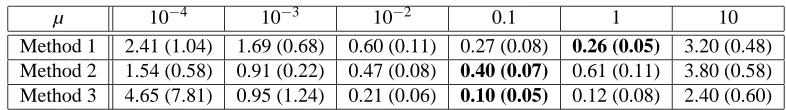
µ 10−4 10−3 10−2 0.1 1 10 Method 1 2.41 (1.04) 1.69 (0.68) 0.60 (0.11) 0.27 (0.08) 0.26 (0.05) 3.20 (0.48) Method 2 1.54 (0.58) 0.91 (0.22) 0.47 (0.08) 0.40 (0.07) 0.61 (0.11) 3.80 (0.58) Method 3 4.65 (7.81) 0.95 (1.24) 0.21 (0.06) 0.10 (0.05) 0.12 (0.08) 2.40 (0.60)

Table 1: Experiment 1: Average mean square error with its standard deviation (in parenthesis) for methods 1 to 3 for different values of the regularization parameterµ(see text for the description). The unit measure for the errors is10−3.

Sµ in equation (5). For this purpose, we use an interior point method, that is, we define, for every

λ= (λ`:`∈INn)∈IRn, the penalized function

F_ν(λ):=Sµ

∑

`∈INn λ`K`

!

−ν

∑

`∈INn

lnλ` (30)

whereνis a positive parameter and solve the variational problem

min

(

F_ν(λ):λ_∈IRn,

∑

`∈INn λ`=1

)

. (31)

Clearly, whenνis small the solution to this problem is close to a minimizer of Sµ, although the penalty term in (30) forces this solution to be interior to the set_{λ:∑`∈INnλ`=1,λ`≥0, `∈INn}.

In order to reach such a minimizer we choose an iteration number R_∈IN and iteratively compute the solution to problem (31) for a decreasing sequence of values of the parameterν. Specifically we set, for r_∈INR,νr=νAr−1 whereνis the initial value ofνand A∈(0,1)is some prescribed pa-rameter. The optimality conditions for problem (31) (see, for example, Rockafellar, 1970; Borwein and Lewis, 2000) are given by the system of non-linear equations

∇F_ν−ηe = 0 −(e,λ) +1 = 0

where e is the vector in IRnall of whose components are one andη_∈IR is the Lagrange multiplier associated to the equality constraint in that problem. We solve these equations by a Newton method (see, for example, Mangasarian, 1994) which consists in iteratively solving the system of linear equations

∇2_F

ν(ˆλ)∆λ−∆ηe = ηˆe₋∇F_ν(λˆ)

−(e,∆_λ) = 0

to obtain the vector∆_λ∈IRmand∆η∈IR, where ˆλand ˆηare the previous values ofλandη. We then update the parameters asλ=ˆλ+α∆_λandη=ηˆ+α∆η, where, in order to insure that λ_∈[0,1]n_, we have setα:=min(1,0.5 max_{α>0 : ˆλ+α∆_λ∈[0,1]_}). In our experiments below we choose R=5,ν=10 and A=0.5.

In both experiments we tried to learn a target function f :[0,2π]_→IR from a set of its samples. In the first experiment we fixed f(x) = 1

10(x+2(e− 8(4

0 1 2 3 4 5 6 7 −0.1 0 0.1 0.2 0.3 0.4 0.5 0.6 0.7

0 1 2 3 4 5 6 7 −0.1 0 0.1 0.2 0.3 0.4 0.5 0.6 0.7

0 1 2 3 4 5 6 7 −0.1 0 0.1 0.2 0.3 0.4 0.5 0.6 0.7

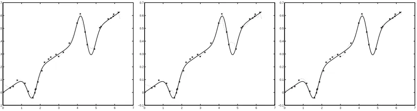
Figure 1: Experiment 1: function learned by method 1 (left), method 2 (center) and method 3 (right). Regu-larization parameter isµ=0.1, the number of training points is50. Solid line is the target function, crosses are the sampled points and the dotted line is the method used. The vertical scale has been reduce

µ 10−4 10−3 10−2 0.1 1 10

Method 1 3.46 (1.39) 3.46( 1.39) 3.45 (1.38) 3.35 (1.35) 2.64 (1.10) 14.1 (10.3) Method 2 4.46 (1.82) 4.46 (1.79) 3.85 (1.18) 3.78 (1.03) 4.00 (1.02) 62.6 (5.11) Method 3 0.52 (0.56) 0.51 (0.56) 0.51 (0.55) 0.51 (0.57) 0.53 (0.63) 3.51 (1.47)

Table 2: Experiment 2: Average mean square error with its standard deviation (in parenthesis) for methods 1 to 3 for different values of the regularization parameterµ(see text for the description). The unit measure for the errors is10−3.

for every x,t_∈[0,2π], we set K`(x,t) = (xt)`−1if`∈ {1,2,3}and K`(x,t) =e−ω`(x−t)

2

if`<sub>∈ {</sub>4,5,6<sub>}</sub> whereω`=28−5(`−4). We generated a training set of fifty points{(xj,yj): j∈IN50} ⊂[0,2π]×IR obtained by sampling f with noise. Specifically, we choose xj uniformly distributed in the interval

[0,2π] and yj = f(xj) +ε with ε also uniformly sampled in the interval [−0.02,0.02]. We then computed on a test set of 100 samples the mean square error between the target function f and the function learned from the training set for different values of the parameter µ. We compare three methods. Method 1 is our proposed approach, method 2 is the average of the kernels, that is we use the kernel K=1

n∑K`and method 3 is the kernel K=K2+K5, the “ideal” kernel, that is, the kernel used to generate the target function. The results are shown in Table 1. Figure 1 shows the function learned by each method.

In our second experiment we fixed f(x) =sin(x)+1

2sin(3x), x∈[0,2π]and K`(x,t) =sin(`x)sin(`t), x,t<sub>∈</sub>[0,2π],`_∈INn. The set up is similar to that in Experiment 1. Method 1 is our proposed ap-proach, method 2 is the average of the kernels and method 3 is the ideal kernel given by K(x,t) =

2

3sin(x)sin(t) + 1

3sin(3x)sin(3t). The noiseεis now uniformly sampled in the interval[−0.2,0.2]. The results are reported in Table 2. Figure 2 shows the function learned by each method.

4.3 Extensions

We discuss some extensions of the problems studied in this paper. The first one that comes to mind is obtained by taking the expectation of the functional (4) with respect to a probability measure P on IRm, that is,

Qav_µ (K):=

Z

0 1 2 3 4 5 6 7 −1.5

−1 −0.5 0 0.5 1 1.5

0 1 2 3 4 5 6 7 −1.5

−1 −0.5 0 0.5 1 1.5

0 1 2 3 4 5 6 7 −1.5

−1 −0.5 0 0.5 1 1.5

Figure 2: Experiment 2: function learned by method 1 (left), method 2 (center) and method 3 (right). Regu-larization parameter isµ=0.1, the number of training points is50. Solid line is the target function, crosses are the sampled points and the dotted line is the method used.

where we indicated the dependency of Qµ(K)on y by writing Qµ(K,y). Since Qµ(K,y)is convex in K for each y∈IRm so is Qav_µ (K). We then minimize Qav_µ (K) over K∈

K

. For the square loss regularization we obtain that

S_µav(K) =µ trace((Kx+µI)−1Σ) (33)

whereΣis the correlation matrix of P. Minimizing the quantity (33) over a convex class

K

may be valuable in image reconstruction and compression where we are provided with a collection of images and we wish to find a good average representation for them. In this case the input x=_{xi: i∈INm} represents the locations of the image pixels. For gray level images we can assume that y_∈[0,1]m_{and therefore we should choose P to have support on[0,1]}m_{. Thus, if{y}`<sub>:`∈IN</sub>

n}is a sample of such images with n<m andΣis the rank n empirical correlation matrix our goal is to find a kernel which well-represents this collection on the average.

Another approach is provided by replacing the average in equation (32) with the maximum over all y with bounded norm, that is, we minimize the functional

Qmax_µ (K):=max_{Qµ(K,y):kyk ≤1}, K∈

K

.

Again, this function is convex in K. In particular, for square loss regularization and the Euclidean norm on IRmwe obtain

max_{Sµ(K,y):kyk ≤1}=max{µ(y,(Kx+µI)−1y):kyk ≤1}=

µ

λmin(Kx) +µ

whereλmin(Kx)is the smallest eigenvalue of the matrix Kx. Consequently, we have that

min_{max_{Sµ(K,y):ky| ≤1}: K∈

K

}=

µ

max_{λmin(Kx): K∈

K

}+µ .

It is well-known thatλmin(Kx)is a concave function of Kx, (see, for example, Marshall and Olkin,

1979, p. 475). Therefore, our results provide an alternate proof of this fact.