A New Approximate Maximal Margin Classiﬁcation Algorithm

(1)

A New Approximate Maximal Margin Classiﬁcation

Algorithm

Dipartimento di Scienze dell’Informazione Universita’ di Milano

Via Comelico 39, 20135 Milano, Italy

Editors:Nello Cristianini, John Shawe-Taylor and Bob Williamson

Abstract

A new incremental learning algorithm is described which approximates the maximal margin hyperplane w.r.t. normp≥2 for a set of linearly separable data. Our algorithm, called alma_p (Approximate Large Margin algorithm w.r.t. normp), takesO

(p−1)

α2_γ2

corrections to separate the data with p-norm margin larger than (1−α)γ, whereγ is the (normal-ized)p-norm margin ofthe data. alma_p avoids quadratic (or higher-order) programming methods. It is very easy to implement and is as fast as on-line algorithms, such as Rosen-blatt’s Perceptron algorithm. We performed extensive experiments on both real-world and artiﬁcial datasets. We compared alma₂ (i.e., alma_p with p = 2) to standard Support vector Machines (SVM) and to two incremental algorithms: the Perceptron algorithm and Li and Long’s ROMMA. The accuracy levels achieved by alma₂ are superior to those achieved by the Perceptron algorithm and ROMMA, but slightly inferior to SVM’s. On the other hand,alma₂is quite faster and easier to implement than standard SVM training algorithms. When learning sparse target vectors, alma_p with p >2 largely outperforms Perceptron-like algorithms, such asalma₂_.

Keywords: Binary Classiﬁcation, Large Margin, Support Vector Machines, On-line Learning

1. Introduction

Vapnik’s Support Vector Machines (SVM) are a statistical model ofdata that simultaneously minimizes model complexity and data ﬁtting error (Vapnik, 1998). SVM have attracted a lot ofinterest and have spurred voluminous work in Machine Learning, both theoretical and experimental. The remarkable generalization ability exhibited by SVM can be explained through margin-based VC theory (e.g., Shawe-Taylor et al., 1998; Anthony and Bartlett, 1999; Vapnik, 1998; Cristianini and Shawe-Taylor, 2000, and references therein).

(2)

Ifan arbitrary norm p is used then such a task turns to a more general mathematical programming problem (e.g., Mangasarian, 1997; Nachbar et al., 1993) to be solved by general purpose (and computationally intensive) optimization methods. This more general task naturally arises in feature selection problems when the target to be learned is sparse (i.e., when the target has many irrelevant features). This is often the case in a number of natural language processing problems (e.g., Golding and Roth, 1996; Dagan et al., 1997).

A fair amount of recent work on SVM centers on finding simple and efficient methods to solve maximal margin hyperplane problems (e.g., Osuna et al., 1997; Joachims, 1998; Friess et al., 1998; Platt, 1998; Kowalczyk, 1999; Keerthi et al., 1999; Li and Long, 1999). This paper follows that trend, giving two main contributions. The first contribution is a new efficient algorithm which approximates the maximal margin hyperplane w.r.t. norm p to any given accuracy. We call this algorithm alma_p (Approximate Large Margin algorithm

w.r.t. norm p). alma_p is naturally viewed as an on-line algorithm, i.e., as an algorithm

which processes the examples one at a time. A distinguishing feature ofalma_p is that its

relevant parameters (such as the learning rate) are dynamically adjusted over time. In this sense, alma_p is a reﬁnement ofthe on-line algorithms recently introduced by Auer et al.

(2001).

On-line algorithms are useful when the examples become available to the learning al-gorithm one at a time, but also when the training set is too large to consider all examples at once. alma₂ (i.e., alma_p with p = 2) is a perceptron-like algorithm; the operations it

performs can be expressed as dot products, so that we can replace them by kernel functions (Aizerman et al., 1964). alma₂ approximately solves the SVM training problem,

avoid-ing quadratic programmavoid-ing. Unlike previous approaches (Cortes and Vapnik, 1995; Osuna et al., 1997; Joachims, 1998; Friess et al., 1998; Platt, 1998), our algorithm operates di-rectly on (an approximation to) the primal maximal margin problem, instead ofits (Wolfe) dual. alma_p is more similar to algorithms such as Li and Long’s ROMMA (Li and Long,

1999) and the one analyzed by Kowalczyk (1999) and Keerthi et al. (1999). However, it seems those algorithms have been speciﬁcally designed for euclidean norm. Unlike those algorithms, alma_p remains computationally eﬃcient when measuring the margin through

a generic norm p.

As far as theoretical performance is concerned, alma₂ achieves essentially the same

bound on the number ofcorrections as the one obtained by a version ofLi and Long’s ROMMA. In the case whenpis logarithmic in the dimension ofthe instance space (Gentile and Littlestone, 1999) alma_p yields results similar to multiplicative algorithms, such as

Littlestone’s Winnow (Littlestone, 1988) and the Weighted Majority algorithm (Littlestone and Warmuth, 1994; Grove et al., 2001). The associated margin-dependent generalization bounds are very close to those obtained by estimators based on linear programming (e.g., Mangasarian, 1968; Anthony and Bartlett, 1999, Chap. 14).

The second contribution ofthis paper is an experimental investigation ofalma_p on

both real-world and artiﬁcial datasets. In our experiments we emphasized the accuracy performance achieved by alma_p as a fully on-line algorithm, i.e., after just one sweep

through the training examples. Following Freund and Schapire (1999), the hypotheses produced by alma_p during training are combined via Helmbold and Warmuth’s (1995)

leave-one out scheme to make a voted hypothesis. We ran alma₂ with kernels on the

(3)

real-world datasets are well-known Optical Character Recognition (OCR) benchmarks. On these datasets we followed the experimental setting described by Cortes and Vapnik (1995), Freund and Schapire (1999), Li and Long (1999) and Platt et al. (1999). We compared our algorithm to standard SVM, to the Perceptron algorithm and to ROMMA. We found thatalma₂ generalizes quite better than both ROMMA and the Perceptron algorithm, but

slightly worse than SVM. On the other hand,alma₂ is as fast and easy to implement as the

other Perceptron-like algorithms. Hence, compared to standard algorithms, training SVM withalma₂ saves a considerable amount oftime.

In the experiments with the artiﬁcial datasets we have been mainly interested in com-paring the accuracy ofPerceptron-like algorithms, such as alma₂, to the accuracy

ofnon-Perceptron-like algorithms, such asalma_p withp >2. When learning sparse target vectors

withalma_p, the performance gap betweenp= 2 andp > 2 is big. This is mainly due to the

diﬀerent convergence speed ofthe two kinds ofalgorithms (see also the paper by Kivinen et al., 1997).

The next section deﬁnes our major notation and recalls some basic preliminaries. In Section 3 we describe alma_p and claim its theoretical properties. Section 4 describes our

experiments. Concluding remarks and open problems are given in the last section.

2. Preliminaries and notation

This section deﬁnes our major notation and recalls some basic preliminaries.

An example is a pair (x, y), where x is aninstance belonging to a giveninstance space

X ⊆ Rn _and _y _{∈ {−}₁_,₊₁_} _{is the binary} _label _{associated with} _x_{. A weight vector} _w ₌

(w1, ..., wn) ∈ Rn represents an n-dimensional hyperplane passing through the origin. It

is natural to associate with w a linear threshold classiﬁer with threshold zero: w : x → sign(w·x) = 1 ifw·x≥0 and =−1 otherwise. Whenp≥1 we denote by||w||_p thep-norm ofw, i.e.,||w||_p = (n_i₌₁|wi|p)1/p(also,||w||∞= limp→∞(

_n

i=1|wi|p)1/p= maxi|wi|). We

say thatqisdualtopif 1_p+1_q = 1 holds. For instance, the 1-norm is dual to the∞-norm and the 2-norm is self-dual. In this paper we assume that pand q are some pair ofdual values, with p ≥ 2. We use p-norms for instances and q-norms for weight vectors. For the sake ofsimplifying notation throughout this paper we use normalized instances ˆx = x/||x||p,

where the norm p will be clear from the surrounding context. The (normalized) p-norm margin (or just the margin, ifpis clear from the context) of a hyperplanewwith||w||_q ≤1 on example (x, y) is defined as yw·xˆ. Ifthis margin is positive1 then w classifies (x, y) correctly. Notice that from Hölder’s inequality we have|w·x| ≤ ||w||ˆ _q||x||ˆ _p ≤1. Hence

yw·xˆ ∈[−1,1].

Our goal is to approximate the maximalp-norm margin hyperplane for a set of examples (the training set). For this purpose, we use terminology and analytical tools from the on-line learning literature. We focus on an on-line learning model introduced by Littlestone (1988) and Angluin (1988). An on-line learning algorithm processes the examples one at a time intrials. In each trial, the algorithm observes an instancex and is required to predict the label y associated with x. We denote the prediction by ˆy. The prediction ˆy combines the current instance x with the current internal state ofthe algorithm. In our case this state

(4)

is essentially a weight vector w, representing the algorithm’s current hypothesis about the maximal margin hyperplane. After the prediction is made, the true value of y is revealed and the algorithm suﬀers aloss, measuring the “distance” between the prediction ˆyand the label y. Then the algorithm updates its internal state.

In this paper the prediction ˆy can be seen as the linear function ˆy=w·xand the loss is a margin-based 0-1 Loss: the loss of w on example (x, y) is 1 if yw·xˆ ≤(1−α)γ and 0 otherwise, for suitably chosen α, γ ∈[0,1]. Therefore, if ||w||_q ≤1 the algorithm incurs positive loss ifand only ifwclassiﬁes (x, y) with (p-norm) margin not larger than (1−α)γ. The on-line algorithms are typically loss driven, i.e., they do update their internal state only in those trials where they suﬀer a positive loss. We call acorrectiona trial where this happens. In the special case whenα = 1 a correction is a mistaken trial and a loss driven algorithm turns to amistake driven (Littlestone, 1988) algorithm.

Throughout the paper we use the subscript t for x and y to denote the instance and the label processed in trial t. We use the subscript k for those variables, such as the algorithm’s weight vector w, which are updated only within a correction. In particular, wk denotes the algorithm’s weight vector afterk−1 corrections (so that w1 is the initial

weight vector). The goal ofthe on-line algorithm is to bound the cumulative loss (i.e., the total number ofcorrections or mistakes) it suﬀers on an arbitrary sequence ofexamples

S = ((x1, y1), ...,(xT, yT)). Consider the special case when S is linearly separable with

marginγ. Ifwe pickα <1 then a bounded loss clearly implies convergence in a ﬁnite number ofsteps to (an approximation of) the maximal margin hyperplane forS. When a training set is linearly separable with margin γ and hyperplane w is such that yw·xˆ ≥(1−α)γ

for any (x, y) in the training set we sometimes say that w is an α-approximation to the maximal margin hyperplane (for that training set).

Remark 1 Our definition of margin is restricted to zero-threshold linear classifiers, i.e., to hyperplanes passing through the origin. The usual definition of margin in SVM literature (Cortes and Vapnik, 1995) actuallyconsiders the more general non-zero threshold linear classifiers. The threshold of an SVM maximal margin hyperplane is sometimes called the

bias term of the SVM. Restricting margin analyses to zero-threshold hyperplanes loses only a constant factor (e.g., Cristianini and Shawe-Taylor, 2000). Nonetheless, in practical applications such a constant factor might make a signiﬁcant diﬀerence.

3. The approximate large margin algorithm alma_p

alma_p is a large margin variant ofthep-norm Perceptron algorithm2 (Grove et al., 2001;

Gentile and Littlestone, 1999), and is similar in spirit to the variable learning rate algorithms introduced by Auer et al. (2001). We analyzealma_pby giving upper bounds on the number

ofcorrections. We do not resort to the prooftechniques developed by (Auer et al., 2001), as they seem to give rise to suboptimal results when applied to the algorithm described here. The theoretical contribution ofthis paper is Theorem 3 below. This theorem has two parts. Part 1 bounds the number ofcorrections in the linearly separable case. In the special case whenp= 2 this bound is very similar to the one proven by Li and Long for a version of

(5)

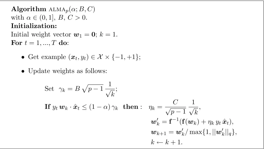
Algorithmalma_p(α;B, C)

withα∈(0,1],B,C >0.

Initialization:

Initial weight vector w1=0;k= 1. For t= 1, ..., T do:

• Get example (x_t, yt)∈ X × {−1,+1}; • Update weights as follows:

Set γk=B

p−1√1

k;

Ifytwk·xˆt≤(1−α)γk then: ηk= √C

p−1 1 √

k,

w_k=f−1(f(w_k) +ηkytxˆt), wk+1=w_k/max{1,||w_k||q},

k←k+ 1.

Figure 1: The approximate large margin algorithmalma_p.

ROMMA (called aggressive ROMMA). Part 2 holds for an arbitrary sequence of examples. A bound which is very close to the one proven by Grove et al. (2001) and Gentile and Littlestone (1999) for the (constant learning rate)p-norm Perceptron algorithm is obtained as a special case.

In order to deﬁne our algorithm, we need to recall the following mappingf (Gentile and Littlestone, 1999) (ap-indexing for f is understood): f : Rn→ Rn,f = (f1, ..., fn), where

fi(w) =

sign(wi)|wi|q−1 ||w||q−2

q

, w= (w1, ..., wn)∈ Rn.

Observe thatp=q= 2 yields the identify function. The (unique) inversef−1off is (Gentile and Littlestone, 1999)f−1 : Rn→ Rn,f−1 = (f1−1, ..., fn−1), where

f_i−1(θ) = sign(θi)|θi|

p−1

||θ||p−2 p

, θ= (θ1, ..., θn)∈ Rn,

namely,f−1is obtained fromfby replacingqwithp. It is easy to check thatf is the gradient ofthe scalar function 1₂|| · ||2_q, whilef−1 is the gradient ofthe (dual) function 1₂|| · ||2_p. The following simple property of f will be useful.

Lemma 2 (Gentile and Littlestone, 1999) The function f maps vectors with a given q -norm to vectors with the same p-norm, i.e., for any w ∈ Rn _{we have} _||_f₍_w₎_||

p = ||w||q.

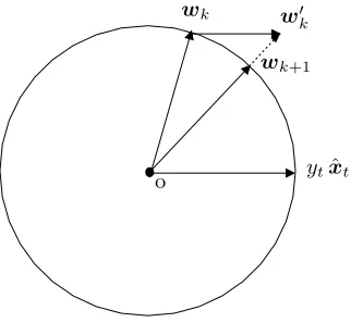
alma_p is described in Figure 1. The algorithm is parameterized by α ∈(0,1], B > 0

(6)

wk _w_k

wk+1

ytxˆt

o

Figure 2: The update rule of alma_p when p=q = 2. The circle is a two-dimensionalW.

hyperplane, while B and C might be considered as tuning parameters. Their use will be made clear in Theorem 3. LetW be theq-norm unit ball, i.e.,W ={w∈ Rn:||w||_q ≤1}.

alma_p maintains a vector w_k of n weights in W. It starts from w₁ = 0. At time t the

algorithm processes example (x_t, yt). Ifthe current weight vector wkclassiﬁes (xt, yt) with

(normalized) margin not larger than (1−α)γkthen a correction occurs. Hereγkis intended

as the current approximation to the unknown maximal margin (denoted byγ∗ in Theorem 3) on the data. The update rule3 _{has two main steps. The ﬁrst step gives} _w

k through the

classical update ofa (p-norm) perceptron-like algorithm (notice, however, that the learning rateηkscales withk, the number ofcorrections occurred so far). The second step giveswk+1

by projecting4 _w

k onto W: wk+1 = wk/||wk||q if ||wk||q >1 and wk+1 = wk otherwise.

The projection step makes the new weight vector w_k+1 belong to W. Figure 2 gives a

graphical representation ofthe update rule.

It is worth discussing at this point howalma_p is qualitatively diﬀerent from previous

on-line algorithms, such as the (p-norm) Perceptron algorithm and ROMMA. First, we notice thatalma_p maintains bounded weight vectors, but it uses a decaying learning rate. This is

actually qualitatively similar to the standard (p-norm) Perceptron algorithm, where weight vectors are unbounded but the learning rate is kept constant. In fact, in both cases later updating instances have less inﬂuence on the direction ofthe current weight vector than earlier instances. On the other hand, unlike the (p-norm) Perceptron algorithm,alma_p is

sensitive to margins, i.e., the current weight vector gets updated even ifthe current margin is positive but smaller than desired. Compared to aggressive ROMMA,alma_p requires the

accuracy parameter α be ﬁxed ahead oftime; ifα is not close to zero, this tends to make

alma_p’s corrections less frequent than aggressive ROMMA’s (see Section 4.2).

3. In the degenerate case thatx_t=0no update takes place.

4. From the proof of Theorem 3 the reader can see that the only way we exploit this projection step is through the condition ||w_k||q ≤ 1 for all k. Therefore if we replaced the update rule w_k₊₁ =

w

(7)

We now claim the theoretical properties of alma_p. The following theorem has two

parts. In part 1 we treat the separable case. Here we prove that a special choice of parametersB and C gives rise to an algorithm which computes anα-approximation to the maximal margin hyperplane, for any given accuraryα. In part 2 we show that ifa suitable relationship betweenB andCis satisﬁed then a bound on the number ofcorrections can be proven in the general (nonseparable) case. The bound ofpart 2 is in terms ofthe margin-based quantity D_γ(u; (x, y)) = max{0, γ −yu·x}ˆ , γ > 0. (Here a p-indexing for D_γ is understood). D_γ is calleddeviationby Freund and Schapire (1999) andlinear hinge lossby Gentile and Warmuth (2001).

Notice that B and C in part 1 do not meet the requirements given in part 2. On the other hand, in the separable case B and C chosen in part 2 do not yield, for any small α, an α-approximation to the maximal margin hyperplane.

Theorem 3 Let X = Rn, W = {w ∈ Rn : ||w||_q ≤ 1}, S = ((x1, y1), ..., (xT, yT)) ∈

(X × {−1,+1})T, and M be the set of corrections of alma_p(α;B, C) running on S (i.e.,

the set of trials t such that ytwk·xˆt≤(1−α)γk).

1. Let γ∗ = max_w_∈Wmin_t=1,...,T ytw·xˆt>0. Thenalmap(α; √

8/α,√2)achieves the following bound5 on|M|:

|M| ≤ 2 (p−1) (γ∗)2

2

α −1

2

+ 8

α −4 =O

p−1

α2₍_γ∗₎2

. (1)

Furthermore, throughout the run of alma_p(α;√8/α,√2) we have γ_k ≥ γ∗. Hence (1) is

also an upper bound on the number of trials tsuch that ytwk·xˆt≤(1−α)γ∗.

2. Let the parameters B and C in Figure 1 satisfythe equation6

C2+ 2 (1−α)B C= 1.

Then for anyu∈ W,alma_p(α;B, C) achieves the following bound on|M|, holding for any

γ >0, where ρ2 = p−1

C2_γ2:

|M| ≤ 1

γ

t∈M

Dγ(u; (xt, yt)) + ρ 2

2 +

ρ4

4 +

ρ2

γ

t∈M

Dγ(u; (xt, yt)) +ρ2.

Observe that when α= 1 the above inequalityturns to a bound on the number of mistaken trials. In such a case the value ofγk (in particular, the value of B) is immaterial, while C

is forced to be 1.

Proof. We assume throughout this proofthat thek-th correction occurs on example (x_t, yt).

We use the following shorthand notation: θ_k = f(w_k), θ_k = f(w_k) = θ_k +ηkytxˆt and

Nk+1 = max{1,||w_k||q}. We now consider the two parts separately. 5. We did not optimize the constants here.

(8)

1. Letγ_k∗=ytu·xˆt, whereu is the maximal margin hyperplane for the whole sequence

S. We study how fast the quantityu·θ_k increases from correction to correction. From the update rule ofFigure 1 we have

u·θk+1= u·θk

+ηkytu·xˆt

Nk+1

= u·θk+ηkγ

∗ k

Nk+1 .

(2)

Observe thatu·θ_k≥0 for any k, since the data are linearly separable.

We need to ﬁnd an upper bound on the normalization factor Nk+1. To this end, we

focus on the squareN_k2+1. By virtue ofLemma 2 we can write

N_k2+1= max{1,||wk||2q}

= max{1,||θ_k||2_p}

= max{1,||θk+ηkytxˆt||2p}.

Furthermore,

||θk+ηkytxˆt||p2 ≤ ||θk||2p+ηk2(p−1) + 2ηkytf−1(θk)·xˆt

=||w_k||2_q+η2_k(p−1) + 2ηkytwk·xˆt ≤1 +η2_k(p−1) + 2 (1−α)ηkγk

= 1 + 2A/k,

where the ﬁrst inequality is essentially proven by Grove et al. (2001) (see also Lemma 2 in the paper by Gentile and Littlestone, 1999), the ﬁrst equality is again an application of Lemma 2, the second inequality derives from Figure 1, and the last equality derives from Figure 1 by setting A= 4/α−3. Thus we conclude that

Nk+1≤

1 + 2A/k.

Now, we set for brevity m =|M|,ρk = √

p−1

γ_k∗ and ρ = √

p−1

γ∗ . Sinceγ∗k and γ∗ are p-norm

margins with γ∗ ≤ γk we have ρk ≥ ρ ≥ 1. We plug the bound on Nk+1 back into (2),

unwrap the resulting recurrence and take into account thatw1 =θ1=0. We yield

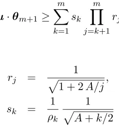
u·θm+1 ≥ m

k=1

sk m

j=k+1

rj,

where

rj =

1

1 + 2A/j,

sk =

1

ρk

1

A+k/2

and the product m_j₌_k₊₁rj is assumed to be 1 if k = m. From H¨older’s inequality and

Lemma 2 it follows that

(9)

Therefore we have obtained: 1≥ m k=1 sk m

j=k+1

rj. (3)

We use this inequality to compute an upper bound on the number ofcorrections m. We proceed by lower bounding the RHS of(3), as a function ofm.

We ﬁrst lower bound sk by 1_ρ √_A₊1_m/₂.Next, considering the product

_m

j=k+1rj, we can

write

−ln

m

j=k+1

rj =

1 2

m

j=k+1

ln

1 +2A

j ≤ 1 2 m

j=k+1

2A j ≤ A _m k 1

jd j

= A lnm

k.

This is equivalent to m_j₌_k₊₁rj ≥

_k

m

A

.Therefore (3) implies

ρ ≥

m

k=1

(k/m)A

A+m/2

≥

_m

k=0

(k/m)A

A+m/2dk

= 1

A+ 1

m

A+m/2.

Solving for m gives

m ≤ ρ

2₍_A_{+ 1)}2

4 +

ρ4₍_A_{+ 1)}4

16 +ρ

2₍_A_{+ 1)}2_A

≤ ρ2(A+ 1)2

4 +ρ(A+ 1)

3/2

ρ2₍_A_{+ 1)}

16 + 1

≤ ρ2(A+ 1)2

4 +ρ(A+ 1)

3/2

ρ2₍_A_{+ 1)}

4 +

2

ρ2₍_A_{+ 1)}

= ρ

2₍_A_{+ 1)}2

2 + 2 (A+ 1) (4)

= 2ρ2

2

α−1

2

+ 8

α −4

= 2 (p−1) (γ∗)2

2

α −1

2

+ 8

(10)

where the third inequality uses√x+ 1≤√x+₂√1

x, f orx >0. This proves that the number

ofcorrections m made by the algorithm is upper bounded as in (1). In order to show that this is also an upper bound on the number oftrials t such that ytwk·xˆt ≤(1−α)γ∗, it

suﬃces to prove thatγk≥γ∗ fork= 1, ..., m. Recalling Figure 1, we see that

γk =

√ 8ρkγ∗k

α√k

≥ √

8ρ γ∗

α√m

≥

√ 8ρ γ∗

α

ρ2 (A+1)2

2 + 2 (A+ 1)

≥ γ∗

α

(A+1)2 16 + A

+1 4

= γ

∗

1−α₄2 ≥ γ∗,

where the second inequality is (4), the third inequality follows from ρ ≥ 1 and the last equality follows from the deﬁnition ofA. This concludes the proofofpart 1.

2. The proofproceeds along the same lines as the proofofpart 1. Thus we only sketch the main steps. Let ube an arbitrary vector inW. We can write

Nk+1u·θk+1 =u·θk+ηkytu·xt, (5)

where

N_k2+1 = max{1,||θk+ηkytxˆt||2p}

≤ max{1,||θk||2p+η2k(p−1) + 2 (1−α)ηkγk ≤ max{1,1 +η_k2(p−1) + 2 (1−α)ηkγk}

= 1 + C

2_{+ 2 (1}₋_α₎_{B C}

k

= 1 + 1

k.

From (5) and the value ofηk we obtain

√

k+ 1u·θ_k+1 ≥

√

ku·θk+ √_pC₋₁ytu·xˆt.

Unwrapping, using the two inequalitiesu·θ_m+1≤1 andytu·xˆt≥γ−Dγ(u; (xt, yt)), and

rearraning yields

√

m+ 1

√

p−1

C +

t∈M

(11)

holding for any γ > 0 and any u ∈ W. Solving for m gives the desired inequality. This concludes the proof.

Some remarks are in order at this point.

Remark 4 It is worth emphasizing that the diﬀerence between parts 1 and 2 in Theorem 3 is mainlytheoretical. For instance, the condition C2 + 2 (1−α)B C = 1 in Part 2 is satisﬁed even by B = ₂√1

α and C = √

α, for any α ∈ (0,1]. It is not hard to see that in

the separable case this setting yields the bounds |M| ≤ 1+

√ 5 2 p−

1

(γ∗)2α and γk ≥γ∗/3 for all

k (independent of α). Hence, if we set α = 1/2 we obtain a hyperplane whose margin on the data is at least γ∗/6 after no more than (1 +√5)₍p−_γ∗₎12 corrections. This degree of data

ﬁtting could be enough for manypractical purposes. In fact, one should not heavilyrelyon Theorem 3 to choose the “best” tuning for B and C in alma_p(α;B, C), since manyof the

constants occurring in the statement of that theorem are just an artifact of our analysis.

Remark 5 When p= 2 the computations performed byalma_p essentiallyinvolve onlydot

products (recall that p = 2 yields q = 2 and f =f−1 = identity). Thus the generalization of alma₂ to the kernel case is quite standard (we just replace everydot product between

instances bya kernel dot product). In fact, the linear combinationw_k+1·xcan be computed

recursively, since

wk+1·x= wk·x

+ηkytxˆt·x

Nk+1 .

Here the denominatorNk+1 equals max{1,||w_k||2}and the norm ||w_k||2 is again computed

recursivelyby

||w

k||22=||wk−1||22/Nk2+ 2ηkytwk·xˆt+η2k,

where the dot product w_k·xˆ_t is taken from the k-th correction (the trial where the k-th weight update did occur), and the normalization of instances xˆ =x/||x||2 is computed as

ˆ

x=x/√x·x.

Remark 6 alma_p with p > 2 is useful when learning sparse hyperplanes, namely those

hyperplanes having only a few relevant components. Gentile and Littlestone (1999) ob-serve that setting p = 2 lnn makes a p-norm algorithm similar to a purelymultiplica-tive algorithm such as Winnow and the Weighted Majorityalgorithm (Littlestone, 1988; Littlestone and Warmuth, 1994). The performance of such algorithms is ruled bya lim-iting pair of dual norms, i.e., the inﬁnitynorm of instances and the 1-norm of weight vectors. Likewise, alma_p with p = 2 lnn becomes a multiplicative approximate

maxi-mal margin classiﬁcation algorithm, where the margin is meant to be an ∞-norm margin. To see this, observe that ||x||_p ≤ n1/p||x||∞ for any x ∈ Rn. Hence p = 2 lnn yields ||x||(2 lnn)≤

√

e||x||∞. Also, ||w||1≤1implies ||w||q ≤1for any q >1. Thus if ||w||1 ≤1

the (2 lnn)-norm margin _||_xy_||w·x

(2 lnn) is actuallybounded from below bythe ∞-norm margin yw·x

||x||∞ divided by √

e. The bound in part 1 of Theorem 3 becomes|M|=O

lnn α2(γ∗)2

, where

γ∗ = max_w:||w||1≤1mint=1,...,T y_||txtw_||·xt_∞. The associated margin-based generalization bounds

(12)

Remark 7 alma_p and its analysis could be modiﬁed to handle the case when the margin

is not normalized, i.e., when the margin of hyperplanew on example (x, y) is deﬁned to be justyw·x. We onlyneed to introduce a new variable, call itXk, which stores the maximal

norm of the instances seen in past corrections, and then normalize the new instance x_t in the update rule by Xk. The resulting algorithm and the corresponding analysis would

be slightlymore complicated than the one we gave in Theorem 3. As a matter of fact, our initial experiments with alma_p-like algorithms were performed with the unnormalized

margin version. Such experiments, which are not reported in this paper, show that the unnormalized margin version ofalma_p is fairlysensitive to example ordering (in particular,

the algorithm is quite sensitive to the position of outliers in the stream of examples). This is one of the reasons whyin this paper we onlytreat the normalized margin version.

4. Experimental results

To see how our algorithm works in practice, we tested it on a number ofclassiﬁcation datasets, both real-world and artiﬁcial. We used alma₂ with kernels on the real datasets

andalma_p withp= 2, 6, 10 withoutkernels on the artiﬁcial ones. The real-world datasets

are well-known OCR benchmarks: the USPS dataset (e.g., Le Cun et al., 1995), the MNIST dataset7, and the UCI Letter dataset (Blake et al., 1998). The artiﬁcial datasets consist ofexamples generated by some random process according to the rules described in Section 4.4.

For the sake ofcomparison, we tended to follow previous experimental setups, such as those described by Cortes and Vapnik (1995), Freund and Schapire (1999), Friess et al. (1998), Li and Long (1999) and Platt et al. (1999). We reduced an N-class problem to a set of N binary problems, according to the so-called one-versus-rest scheme. That is, we trained the algorithms once for each of the N classes. When training on the i-th class all the examples with label i are considered positive (labelled +1) and all other examples are negative (labelled −1). Classification is made according to the maximum output of the N binary classifiers. There are many other ways ofcombining binary classifiers into a multiclass classifier. We refer the reader to the work by Dietterich and Bakiri (1995), Platt et al. (1999), Allwein et al. (2000) and to references therein. Yet another method for facing multiclass classification (which does not explicitly reduce to binary) is mentioned in Section 5.

Our experimental results are summarized in Tables 1 through 6 and in Figures 3, 4 and 5. Following Freund and Schapire (1999), the output ofa binary classiﬁer is based on either thelasthypothesis produced by the algorithms (denoted by “last” throughout this section) or Helmbold and Warmuth’s (1995) leave-one-out voted hypothesis (denoted by “voted”). In our experiments we actually used the variant called average by Freund and Schapire (1999). We denote it by “average” or “avg”, for brevity. This variant gave rise to slight accuracy improvements compared to “voted”.8 When using “last”, the output ofthe i-th 7. It can be downloaded from Y. LeCun’s home page: http://www.research.att.com/∼yann/ocr/mnist/. 8. Freund and Schapire (1999) seem to use the average variant without any theoretical justiﬁcation. When

using margin sensitive classiﬁcation algorithms, such asalma_p_withα <_{1, one can prove a bound on}

(13)

binary classiﬁer on a new instance xis

output_i(x) =w(i)

m(i)+1·x,

where w(i)

m(i)+1 is the last weight vector produced during training by the i-th classiﬁcation

algorithm (namely, after m(i) corrections); when using “voted” or “avg” we need to store the sequence ofprediction vectors w(₁i), w₂(i), ..., w(i)

m(i)+1, as well as the number oftrials

the corresponding prediction vector survives until it gets updated. Let us denote by c(_ki)

the number oftrials the k-th weight vector ofthe i-th classiﬁer survives. Then ifwe use “voted” the output ofthe i-th classiﬁer on instance xis

output_i(x) =

m(i)+1 k=1

c(_ki)sign(w(_ki)·x);

ifwe use “avg” the output ofthei-th classiﬁer on instance xis

output_i(x) =  m

(i)₊₁

k=1

c(_ki)w(_ki)  _·_x_.

In all cases the predicted label ˆy associated withxis

ˆ

y= argmax_i₌₁_...N output_i(x).

We trained the algorithms by cycling up to 3 times (“epochs”) over the training set. All the results shown in Tables 1–6 and in Figures 3–5 are averaged over 10 random permuta-tions ofthe training sequences.

In Tables 1–6 the columns marked “TestErr” give the fraction of misclassiﬁed examples in the test set. The columns marked “Correct” (or “Corr”, for brevity) give the total number ofcorrections occurred in the training phase for the N labels (recall that for Perceptron and alma_p withα= 1 a correction is the same as a mistaken trial).

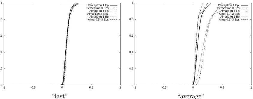
In Figures 3–5 we plotted a number of margin distribution graphs (Schapire et al., 1998) yielded when runningalma_p on various datasets. For binary classiﬁcation tasks the

margin distribution ofa (binary) classifier w with ||w||_q ≤ 1 is the fraction of examples (x, y)∈ X × {−1,+1} in the training set whose margin yw·xˆ is at mosts, as a function ofs∈[−1,+1]. For anN-class problem solved via the one-versus-rest scheme, it is natural to define the margin as the difference between the output ofthe classifier associated with the correct label and the maximal output ofany other classifier. This value lies in [−1,+1] once weight vectors and instances are properly normalized. Also, the margin is positive if and only ifthe example is correctly classified.

In our experiments no special attention has been paid to tune scaling factors and/or noise-control parameters. As far as parametersB and C is concerned, we have set C=√2 (as in Theorem 3, part 1) andB = _α1, whereαis chosen in the set{1.0, 0.95, 0.9, 0.8, 0.5}. Notice that with this parameterization the weight update condition ytwk·xˆt≤(1−α)γk

in Figure 1 actually becomes ytwk·xˆt ≤β √

p−1 √

(14)

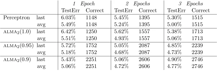
1 Epoch 2 Epochs 3 Epochs

TestErr Correct TestErr Correct TestErr Correct Perceptron last 6.03% 1148 5.45% 1395 5.30% 1515

avg 5.49% 1148 5.24% 1395 5.00% 1515

alma₂(1.0) last 6.42% 1250 5.62% 1557 5.38% 1713

avg 5.51% 1250 4.93% 1557 5.06% 1713

alma₂(0.95) last 5.72% 1752 5.05% 2087 4.85% 2239

avg 5.18% 1752 4.68% 2087 4.73% 2239

alma₂(0.9) last 5.43% 2251 5.06% 2606 4.90% 2746

avg 5.06% 2251 4.72% 2606 4.77% 2746

Table 1: Experimental results on USPS database. We used Gaussian kernels with width

σ = 3.5. “TestErr” denotes the fraction of misclassiﬁed patterns in the test set, while “Correct” denotes the total number oftraining corrections for the 10 labels. alma₂(α) is

shorthand foralma₂(α;1

α, √

2). Recall that averaging takes place during the testing phase. Thus the number ofcorrections of“last” is the same as the number ofcorrections of“avg”.

Below we are using the shorthandalma_p(α) to denotealma_p(α;1

α, √

2). Thus, for example,

alma_p(1.0) denotesalma_p(1; 1,√2).

We made no preprocessing on the data (beyond the implicit preprocessing performed by the kernels). All our experiments have been run on a PC with a single PentiumIII MMX processor running at 447 Mhz. The running times we will be mentioning are measured on this machine.

The rest ofthis section describes the experiments in some detail.

4.1 Experiments with USPS dataset

The USPS (US Postal Service) dataset has 7291 training patterns and 2007 test patterns. Each pattern is a 16×16 vector representing a digitalized image ofa handwritten digit, along with a {0,1,...,9}-valued label. The components ofsuch vectors lie in [−1,+1].

This is a well-known SVM benchmark. The accuracy results achieved by SVM range from 4.2% (obtained by Cortes and Vapnik, 1995, after suitable data smoothing) to 4.4% (reported by Sch¨olkopfet al., 1999) to 4.7% (reported by Platt et al., 1999, with no data preprocessing). The best accuracy results we are aware ofare those obtained by Simard, et al. (1993). They yield a test error of2.7% by using a notion ofdistance between patterns that encodes speciﬁc prior knowledge about OCR problems, such as invariance to translation and rotation.

We ran both the Perceptron algorithm and alma₂. Following Sch¨olkopfet al. (1997,

1999), Platt et al. (1999) and Friess et al. (1998), we used the Gaussian kernel

K(x,y) = exp

−||x−y||22 2σ2

. To choose the best width σ, we ran the Perceptron algo-rithm and alma₂(1.0) for one epoch. We used 5-fold cross validation on the training set

across the range [0.5,10.0] with step 0.5. The best σ for both algorithms turned out to be

(15)

digit 0 1 2 3 4 5 6 7 8 9

alma₂(1.0)

1 Epoch Corr 99 46 129 147 142 156 101 102 169 159

SV 99 46 129 147 142 156 101 102 169 159

2 Epochs Corr 121 58 164 183 174 195 127 128 206 201

SV 121 55 159 182 168 193 126 124 202 195

3 Epochs Corr 138 67 174 204 193 208 145 137 228 219

SV 138 61 173 197 184 205 142 132 224 210

alma₂(0.95)

1 Epoch Corr 149 79 192 203 190 214 148 144 226 207

SV 149 79 192 203 190 214 148 144 226 207

2 Epochs Corr 176 94 226 242 226 255 174 168 277 249

SV 175 89 224 238 221 253 173 163 272 243

3 Epochs Corr 186 105 235 256 243 273 188 184 297 272

SV 185 94 233 250 234 268 184 173 288 254

alma₂(0.9)

1 Epoch Corr 200 110 246 255 243 279 193 182 287 256 SV 200 110 246 255 243 279 193 182 287 256

2 Epochs Corr 224 128 284 294 286 320 224 209 331 306 SV 223 123 282 290 280 314 220 201 323 294

3 Epochs Corr 230 137 294 312 300 334 235 226 349 329 SV 229 126 288 305 289 328 227 214 337 309

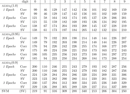
SVM (SV) 219 91 316 309 288 340 213 206 304 250

Table 2: Experimental results on USPS database. “Corr” denotes the total number of training corrections for the 10 labels, while “SV” denotes the number of “support vectors” for the 10 labels. alma₂(α) is shorthand foralma₂(α;1

α, √

(16)

using a Gaussian kernel makes the normalization ofinstances ˆx=x/||x||2 immaterial, since

K(x,x) = 1 for any x.

Table 1 gives test error and number ofcorrections for the Perceptron algorithm and

alma₂ with diﬀerent values of α. Table 2 gives statistics for alma₂ on the ten digits.

Here “Corr” denotes the number ofcorrections while “SV” denotes the number of“support vectors”, i.e., the number ofexamples that are actually involved in computing the prediction function for each of the ten classes. For the sake of comparison, we also give the number ofsupport vectors yielded by SVM, as reported by Sch¨olkopfet al. (1999). The standard deviations related to our averages are reasonably small; those concerning test errors are about 0.12%.

On this dataset alma₂(1.0) and the Perceptron algorithm perform comparably. The

accuracy of alma₂(α) improves signiﬁcantly when we shrink the value of α, whereas the

computed solution gets less and less sparse.

As in the experiments performed by Freund and Schapire (1999) and Li and Long (1999), the accuracy ofthe classiﬁers tends to get better as we increase the number of training epochs. However, training alma₂ “avg” for more than two epochs seems to hurt

performance somewhat. This might be due to the fast convergence of this algorithm (notice that the accuracy obtained by SVM is quite close).

We found the accuracy of 5.06% for alma₂(0.9) “avg” fairly remarkable, considering

that it has been obtained by sweeping through the examples just once for each of the ten classes. Indeed, the algorithm is quite fast: training for one epoch the ten binary classiﬁers of alma₂(0.9) takes on average only 6.5 minutes.

The reader might want to compare this performance to the similar accuracy of 5.00% achieved by the “average” Perceptron algorithm run for three epochs. Despite Perceptron’s solution is sparser than alma₂(0.9)’s, it is worth saying that running Perceptron for three

epochs takes about twice as long as training alma₂(0.9) for one epoch.

We plot in Figure 3 some ofthe margin distribution graphs obtained. The value ofthe curves at a given point s∈[−1,+1] gives the fraction of patterns in the training set whose margin (after training) is at mosts. alma₂(0.9) tends to increase the number ofexamples

with a strictly positive margin. This is actually more evident with the “average” variant (plots on the right) than with the “last” variant (plots on the left).

4.2Experiments with the MNIST dataset

Each example in MNIST dataset is a 28×28 matrix, along with a {0,1,...,9}-valued label. Each entry in this matrix is a value in{0,1,...,255}, representing a grey level. The database has 60000 training examples and 10000 test examples.

The best accuracy results for this dataset are those obtained by Le Cun et al. (1995) through boosting on top ofthe neural net LeNet4. They reported a test error rate of0.7%. A soft margin SVM achieved an error rate of 1.1% (Cortes and Vapnik, 1995).

(17)

0 0.2 0.4 0.6 0.8 1

-1 -0.5 0 0.5 1

Perceptron 1 Ep Perceptron 3 Eps Alma(1.0) 1 Ep Alma(1.0) 3 Eps Alma(0.9) 1 Ep Alma(0.9) 3 Eps

0 0.2 0.4 0.6 0.8 1

-1 -0.5 0 0.5 1

Perceptron 1 Ep Perceptron 3 Eps Alma(1.0) 1 Ep Alma(1.0) 3 Eps Alma(0.9) 1 Ep Alma(0.9) 3 Eps

“last” “average”

Figure 3: Some ofthe margin distribution functions yielded by the Perceptron algorithm and byalma₂, run for 1 and 3 epochs on USPS dataset.

the kernel to 4. According to Freund and Schapire (1999) this choice was best. The same choice was made by Cortes and Vapnik (1995) and Li and Long (1999). Later on we found that signiﬁcant improvements could be obtained by a largerd.

We give results for alma₂ withd= 4,5,6. We have not investigated any careful tuning

of scaling factors. In particular, we have not determined the best instance scaling factors

for our algorithm (this corresponds to using the kernel K(x,y) = (1 +x·y/s)d). In our experiments we sets= 255. This was actually the best choice made by Li and Long (1999) for the Perceptron algorithm.

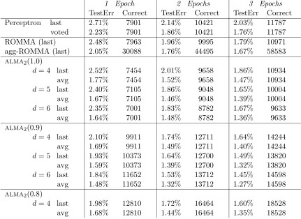
The experimental results are given in Tables 3 and 4. Table 3 gives test error and number ofcorrections for the Perceptron algorithm, ROMMA andalma₂(α) withα= 1.0, 0.9, 0.8.

The ﬁrst four rows ofTable 1 summarize some ofthe results obtained by Freund and Schapire (1999), Li and Long (1999) and Li (2000). The ﬁrst two rows refer to the Percep-tron algorithm, while the third and the fourth rows refer to the original ROMMA9 and the best noise-controlled version ofROMMA, called “aggressive ROMMA”. Both the Percep-tron algorithm and ROMMA have been run with a degree 4 polynomial kernel. Our own experimental results are given in the subsequent rows.

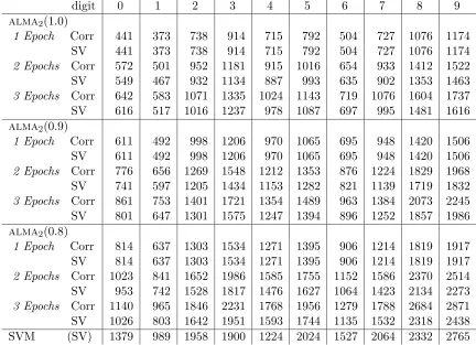
Table 4 is analogous to Table 2 and refers to alma₂ with a degree 4 polynomial kernel.

In the last row ofTable 4 we give the number ofsupport vectors yielded by the soft-margin SVM employed by Cortes and Vapnik (1995). Again, the standard deviations about the averages we report in these tables are not large. Those concerning test errors range in (0.03%, 0.09%).

Among these Perceptron-like algorithms, alma₂ “avg” seems to be the most accurate.

Again, we would like to emphasize the good accuracy performance yielded byalma₂on the

ﬁrst epoch. Notice that if d= 6 alma₂(0.9) “avg” gets 1.48%.

(18)

voted 2.23% 7901 1.86% 10421 1.76% 11787

ROMMA (last) 2.48% 7963 1.96% 9995 1.79% 10971

agg-ROMMA (last) 2.05% 30088 1.76% 44495 1.67% 58583

alma₂(1.0)

d= 4 last 2.52% 7454 2.01% 9658 1.86% 10934

avg 1.77% 7454 1.52% 9658 1.47% 10934

d= 5 last 2.40% 7105 1.86% 9048 1.65% 10004

avg 1.67% 7105 1.46% 9048 1.39% 10004

d= 6 last 2.35% 7001 1.83% 8782 1.67% 9633

avg 1.64% 7001 1.48% 8782 1.36% 9633

alma₂(0.9)

d= 4 last 2.10% 9911 1.74% 12711 1.64% 14244

avg 1.69% 9911 1.49% 12711 1.40% 14244

d= 5 last 1.93% 10373 1.64% 12700 1.49% 13820 avg 1.59% 10373 1.39% 12700 1.32% 13820

d= 6 last 1.84% 11652 1.53% 13712 1.45% 14598 avg 1.48% 11652 1.32% 13712 1.27% 14598

alma₂(0.8)

d= 4 last 1.98% 12810 1.72% 16464 1.60% 18528 avg 1.68% 12810 1.44% 16464 1.35% 18528

Table 3: Experimental results on MNIST database. The results have been obtained through the polynomial kernelK(x,y) = (1 +x·y/255)d. The Perceptron algorithm and ROMMA use d = 4, while alma₂ uses d = 4,5,6. “TestErr” denotes the fraction of misclassiﬁed

patterns in the test set, while “Correct” denotes the total number oftraining corrections for the 10 labels.

alma₂ is quite fast. Training for one epoch the ten binary classiﬁers ofalma₂(1.0) with d= 4 takes on average 2.3 hours and the corresponding testing time is on average about 40 minutes; training for one epoch the ten binary classiﬁers ofalma₂(0.9) withd= 6 takes on

average 4.3 hours, while testing takes on average 1.2 hours.

There seems to be no big diﬀerence in accuracy between alma₂(0.9) and alma₂(0.8)

when d = 4. This suggested us not to run alma₂(0.8) with d > 4. Also, we have not

run alma₂ for more than 3 epochs. But it seems reasonable to expect the accuracy of alma₂(0.9) “avg” and alma₂(0.8) “avg” to get closer and closer to the one achieved by

SVM.

4.3 Experiments with UCI Letter dataset

(19)

digit 0 1 2 3 4 5 6 7 8 9

alma₂(1.0)

1 Epoch Corr 441 373 738 914 715 792 504 727 1076 1174 SV 441 373 738 914 715 792 504 727 1076 1174

2 Epochs Corr 572 501 952 1181 915 1016 654 933 1412 1522 SV 549 467 932 1134 887 993 635 902 1353 1463

3 Epochs Corr 642 583 1071 1335 1024 1143 719 1076 1604 1737 SV 616 517 1016 1237 978 1087 697 995 1481 1616

alma₂(0.9)

1 Epoch Corr 611 492 998 1206 970 1065 695 948 1420 1506 SV 611 492 998 1206 970 1065 695 948 1420 1506

2 Epochs Corr 776 656 1269 1548 1212 1353 876 1224 1829 1968 SV 741 597 1205 1434 1153 1282 821 1139 1719 1832

3 Epochs Corr 861 753 1401 1721 1354 1489 963 1384 2073 2245 SV 801 647 1301 1575 1247 1394 896 1252 1857 1986

alma₂(0.8)

1 Epoch Corr 814 637 1303 1534 1271 1395 906 1214 1819 1917 SV 814 637 1303 1534 1271 1395 906 1214 1819 1917

2 Epochs Corr 1023 841 1652 1986 1585 1755 1152 1586 2370 2514 SV 953 742 1528 1817 1476 1627 1064 1423 2134 2273

3 Epochs Corr 1140 965 1846 2231 1768 1956 1279 1788 2684 2871 SV 1026 803 1642 1951 1593 1744 1135 1532 2318 2438 SVM (SV) 1379 989 1958 1900 1224 2024 1527 2064 2332 2765

(20)

avg 4.83% 5010 3.70% 6131 3.33% 7001

alma₂(1.0) last 7.00% 5484 4.92% 6685 4.45% 7194

avg 4.82% 5484 3.87% 6685 3.47% 7194

alma₂(0.9) last 4.90% 8312 3.85% 9644 3.50% 10178

avg 3.85% 8312 3.10% 9644 3.02% 10178

alma₂(0.8) last 4.20% 11258 3.55% 13003 3.27% 13673

avg 3.60% 11258 2.97% 13003 2.80% 13673

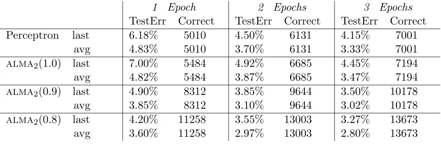
Table 5: Experimental results on UCI Letter database. We used a “poly-Gaussian” kernel (see main text). “TestErr” denotes the fraction of misclassiﬁed patterns in the test set, while “Correct” denotes the total number oftraining corrections for the 26 labels.

extracted from raster scan images ofmachine printed letters of20 diﬀerent fonts. The attributes have values in {0, 1, ..., 15}. A standard split is to consider the ﬁrst 16000 patterns as training set and the remaining 4000 patterns as test set.

The best accuracy results we are aware ofare those obtained by Schwenk and Bengio (2000) by boosting suitable neural network architectures. They reported an error rate of 1.5%. According to Platt et al. (1999), a Gaussian kernel SVM achieves 2.2%. This accuracy diﬀerence might actually be due to diﬀerent preprocessing.

This is a dataset where Perceptron-like algorithms such asalma₂did not work as well as

we would have liked. We ran both the Perceptron algorithm andalma₂. Both algorithms

exhibited a somewhat slow convergence. Besides, they both failed to converge to SVM’s accuracy level. We tried to speed up convergence by using a “poly-Gaussian” kernel ofthe

form K(x,y) =

1 + exp

−||x−y||22 2σ2

_d

. This kernel corresponds to a linear combination of dGaussian kernels with diﬀerent width parametersσ. We set d= 5 to make the kernel ﬂexible enough. Again, in order to determine the best σ, we ran the Perceptron algorithm and alma₂(1.0) for one epoch, using 4-fold cross-validation on the training set across the

range [0.5, 10.0], with step 0.5. The best σ for Perceptron was 4.0, while the best σ for

alma₂ turned out to be 3.0. The experiments are summarized in Table 5, where only the

best results are shown.

The conclusions we can draw from this table are similar to those for Table 1 and Table 3. The main diﬀerence is that the test error achieved by alma₂ after one epoch (alma₂(0.8)

“avg” achieves 3.60%) is signiﬁcantly worse than SVM’s (2.2%). The accuracy of alma₂

tends to improve after the ﬁrst epoch (it reaches 2.80% after three epochs), but it stabilizes around 2.7%, no matter how many epochs one trains the algorithm for. We observed a similar behavior with the Perceptron algorithm (with an even slower convergence). This phenomenon might be due to the lack ofSVM’s bias term.

As far as running time is concerned, training alma₂(1.0) for one epoch takes about 2.5

(21)

4.4 Experiments with alma_p on artiﬁcial datasets

We tested alma_p, p≥2, without kernels on medium-size artiﬁcial datasets. The datasets

are about binary classification tasks and have been generated at random according to the following rules. We first generated a target vector u ∈ {−1,0,+1}300, where the first s

components are selected independently at random in{−1,+1} and the remaining 300−s

components are 0. The valuesis intended as a measure ofthe sparsityoftarget vectoru. In our experiments we set s = 3, 10, 100, 300. We also added labelling noise with rate

(. In our experiments (= 0.0, 0.05, 0.10, 0.15. For a given target vector u and a given noise rate(, we randomly generated 10000 training examples and 10000 test examples. The instance vectors x_t have 300 components with values chosen in [−1,+1]. The training set is generated as follows. We pickedx_t∈[−1,+1]300 at random. Ifu·x_t≥1 then a +1 label is associated with x_t. If u·x_t ≤ −1 then a −1 label is associated with x_t. The labels so obtained are then ﬂipped with probability (. If |u·x_t|<1 then x_t is rejected and a new vectorx_tis drawn. The test set instancesx_tare again chosen at random in [−1,+1]300, the corresponding labels equal10 sign(u·x_t). We did not force a large margin on the test set.

On each ofthese 4×4 = 16 datasets we ran alma_p₍_α_{) (both “last” and “avg”) for one}

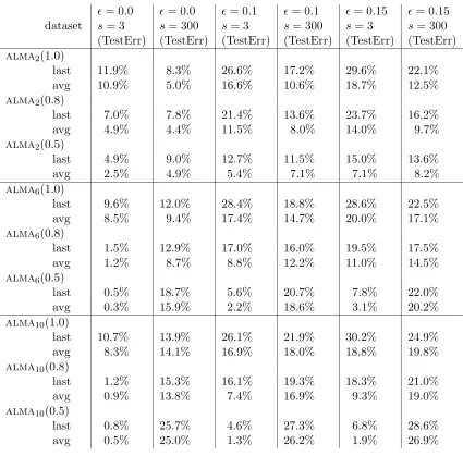
epoch, with p = 2, 6, 10 and α = 1.0, 0.9, 0.8, 0.5. The accuracy results (test errors) are shown in Table 6. These experiments had the purpose ofinvestigating the behavior of

alma_p on extreme scenarios. The diﬀerences in performance are big and sometimes even

huge. In Table 6 we report what we believe are some ofthe most interesting results. We picked 6 out ofthe 16 datasets. The columns are marked according to the values of( and

s.

On sparse target datasets (s = 3 in Table 6) alma₆ and alma₁₀ largely outperform alma₂. On these datasets the accuracy ofall algorithms improves as α is made smaller.

Correspondingly, the number ofcorrections (not shown in Table 6) increases. Like in the experiments ofthe previous subsections, there is a natural trade-oﬀ between the number of corrections the algorithms make and the accuracy ofthe resulting hypotheses. To give an idea ofthis trade-oﬀ, we report three results: on the “(= 0.0, s= 3” dataset alma₂(1.0)

makes on average 142 corrections, while alma₂(0.5) makes 2720 corrections; on the same

dataset, alma₁₀(1.0) makes on average only 14 corrections, whereas alma₁₀(0.5) makes

1050; on the “( = 0.15, s = 3” dataset alma₁₀(1.0) makes on average 2656 corrections

while alma₁₀(0.5) makes on average 3594 corrections. The reader might want to compare

the accuracy results for these three cases. For any given value of α, there is essentially no diﬀerence between alma₁₀(α) and alma₆(α) (the test errors shown in Table 6 are

meaningful up to about 1%).

On dense target datasets (s = 300) alma_p(α) with p = 2 is best. Again, accuracy

improves by shrinkingα, but it degrades as we increasep.

In Figure 4 we plot the margin distribution graphs obtained on 4 ofthe 16 datasets generated. In these plots we put emphasis on the comparison between the two extreme cases α = 1.0 and α = 0.5. The performance gap between alma₂(α) and alma₆(α) on

the two “s = 3” datasets (plots on the left) is clearly reﬂected by the diﬀerent behavior ofthe corresponding margin distribution functions. The plots on the right, on the other

(22)

(= 0.0 (= 0.0 (= 0.1 (= 0.1 (= 0.15 (= 0.15 dataset s= 3 s= 300 s= 3 s= 300 s= 3 s= 300

(TestErr) (TestErr) (TestErr) (TestErr) (TestErr) (TestErr)

alma₂(1.0)

last 11.9% 8.3% 26.6% 17.2% 29.6% 22.1%

avg 10.9% 5.0% 16.6% 10.6% 18.7% 12.5%

alma₂(0.8)

last 7.0% 7.8% 21.4% 13.6% 23.7% 16.2%

avg 4.9% 4.4% 11.5% 8.0% 14.0% 9.7%

alma₂(0.5)

last 4.9% 9.0% 12.7% 11.5% 15.0% 13.6%

avg 2.5% 4.9% 5.4% 7.1% 7.1% 8.2%

alma₆(1.0)

last 9.6% 12.0% 28.4% 18.8% 28.6% 22.5%

avg 8.5% 9.4% 17.4% 14.7% 20.0% 17.1%

alma₆(0.8)

last 1.5% 12.9% 17.0% 16.0% 19.5% 17.5%

avg 1.2% 8.7% 8.8% 12.2% 11.0% 14.5%

alma₆(0.5)

last 0.5% 18.7% 5.6% 20.7% 7.8% 22.0%

avg 0.3% 15.9% 2.2% 18.6% 3.1% 20.2%

alma₁₀(1.0)

last 10.7% 13.9% 26.1% 21.9% 30.2% 24.9%

avg 8.3% 14.1% 16.9% 18.0% 18.8% 19.8%

alma₁₀(0.8)

last 1.2% 15.3% 16.1% 19.3% 18.3% 21.0%

avg 0.9% 13.8% 7.4% 16.9% 9.3% 19.0%

alma₁₀(0.5)

last 0.8% 25.7% 4.6% 27.3% 6.8% 28.6%

avg 0.5% 25.0% 1.3% 26.2% 1.9% 26.9%

Table 6: Results ofexperiments on artiﬁcially generated datasets. Recall that(denotes the amount oflabelling noise, whilesis the number ofnonzero components oftarget vectoru.

hand, are somewhat less informative. When learning a dense (“s = 300”) target, a single training epoch is probably not suﬃcient to diﬀerentiate algorithms’ performance through their margin properties.

(23)

0 0.2 0.4 0.6 0.8 1

-1 -0.5 0 0.5 1

p = 2, alpha = 1.0 p = 2, alpha = 0.5 p = 6, alpha = 1.0 p = 6, alpha = 0.5

0 0.2 0.4 0.6 0.8 1

-1 -0.5 0 0.5 1

Noise rate(= 0.0, sparsitys= 3. Noise rate(= 0.0, sparsity s= 300.

0 0.2 0.4 0.6 0.8 1

-1 -0.5 0 0.5 1

0 0.2 0.4 0.6 0.8 1

-1 -0.5 0 0.5 1

Noise rate(= 0.1, sparsity s= 3. Noise rate(= 0.1, sparsity s= 300.