An interval mixed-integer non-linear programming model to support regional electric power systems planning with CO2 capture and storage under uncertainty

(1)

R E S E A R C H

Open Access

An interval mixed-integer non-linear

programming model to support regional electric

power systems planning with CO

₂

capture and

storage under uncertainty

X.Q. Wang

1

, G.H. Huang

1,2*

and Q.G. Lin

3

Abstract

Background:Electric generating capacity expansion has been always an essential way to handle the electricity

shortage, meanwhile, greenhouse-gas (GHG) emission, especially CO2, from electric power systems becomes crucial considerations in recent years for the related planners. Therefore, effective approach to dealing with the tradeoff between capacity expansion and carbon emission reduction is much desired.

Results:In this study, an interval mixed-integer non-linear programming (IMINLP) model was developed to assist

regional electric power systems planning under uncertainty. CO2capture and storage (CCS) technologies had been introduced to the IMINLP model to help reduce carbon emission. The developed IMINLP model could be

disassembled into a number of ILP models, then two-step method (TSM) was used to obtain the optimal solutions. A case study was provided for demonstrating applicability of the developed method.

Conclusions:The results indicated that the developed model was capable of providing alternative decisions based

on scenario analysis for electricity planning with consideration of CCS technologies. The IMINLP model could provide an effective linkage between carbon sequestration and electric generating capacity expansion with the aim of minimizing system costs.

Keywords:Electric power planning, GHG emission, CCS technologies, Uncertainty, Optimization model

Introduction

Due to rapidly growing population and booming econ-omy, electricity shortage is becoming a significant chal-lenge towards regional electric power systems (REPS). Electric generating capacity planning is obviously an es-sential approach to deal with this issue. The traditional aim of an electric power utility has focused on provi-ding an adequate supply of electric energy at minimum cost (Karaki et al. 2002). In fact, such a planning deci-sion is considerably complicated as it is not only invol-ving a large number of social, economic, political and technical factors and their interactions, but also

coupled with complex temporal and spatial variabilities (Lin and Huang 2009b). Moreover, global climate change induced by the emission of greenhouse gas (GHG) may pose challenges to the fundamental struc-ture of electric power systems (Hidy and Spencer 1994; Wise et al. 2007); meanwhile, the vulnerability of energy sources, in particular of renewable sources, raises the need to identify sustainable adaptation measures (Merrill and Wood 1991; de Lucena et al. 2010). Therefore, effective planning for electric power system under various uncer-tainties and dynamic complexities is much desired.

Previously, a number of studies were conducted for planning electric power system expansion. For example, Sanghvi and Shavel (1984) developed a linear constraint that can be incorporated explicitly into a linear pro-gramming (LP) formulation of an electric utility’s cap-acity expansion planning problem. Zafer Yakin and

* Correspondence:[email protected]

1

Institute for Energy, Environment and Sustainable Communities, University of Regina, Regina, Saskatchewan, Canada S4S 0A2

2

Institute for Energy, Environment and Sustainability Research, UR-NCEPU, North China Electric Power University, Beijing 102206, China

Full list of author information is available at the end of the article

(2)

McFarland (1987) introduced a non-linear program-ming approach for long-range generating capacity ex-pansion planning. In recent years, considerable efforts were made to develop energy systems planning models with consideration of GHG emission reduction under uncertainty (Voropai and Ivanova 2002; Cai et al. 2009a, b; Lin et al. 2010; Wu et al. 2010; Yan et al. 2010). Cao et al. (2010) employed an integer program-ming model with random-boundary intervals for planning municipal power systems, and Li et al. (2010) used a multistage interval-stochastic integer linear pro-gramming approach to deal with uncertainties existing in regional power system planning. Lin and Huang (2009a, b, 2010) developed a series of inexact energy systems planning models for supporting GHG emission management and sustainable renewable energy devel-opment under uncertainty.

The previous studies emphasized on the planning of either electric power systems or entire energy systems by regarding the GHG emission reduction as a single constraint. Studies on how to apply new technologies related to CO2capture and storage (CCS) or adjust the electricity generating structure, however, have hardly been covered in their models. CCS is the key technology that reduces carbon emissions from coal-fired power plants, and as such is essential since coal is at present the predominant fuel for electricity and responsible for no less than 40% of global CO2emissions (de Coninck et al. 2009). In addition, CCS is regarded as one of the

most promising technologies for reducing GHG emis-sions from fossil fuel use (Mitrovic and Malone 2011). As a result, it is necessary to incorporate CCS technology into electric power systems management and provide the decision makers with comprehensive optimization solutions by assessing its contribution to CO2 emission deduction and impacts on electricity generation and capacity expansion.

Therefore, the objective of this study is to develop an interval mixed-integer non-linear programming (IMINLP) model to support regional electric power sys-tems planning with consideration of CO2 capture and storage technologies within an optimization framework. The main tasks will consist of (i) modeling of a typical electric power system in regional level in collaboration with electricity generation, capacity expansion, applica-tion of CCS technologies, sustainability and reliability of electricity energy market, and fluctuated electricity demands; (ii) integrating interval-parameter program-ming techniques into the developed model to formulate an IMINLP model; and (iii) applying the IMINLP model to a regional electric power system to demonstrate its ef-fectiveness in providing decision bases in terms of elec-tricity planning with CCS technologies.

Development of IMINLP model

A typical electric power system is related to a number of energy supply, energy conversion and electricity de-mand activities (shown in Figure 1). The side of

C o a l fir e d p o w e r

N a t r u a l g a s f ir e d p o w e r

H y d r o p o w e r

W in d p o w e r

P u lv e r is e d c o a l f ir e d

te c h n o lo g y

In te g r a te d g a s ific a t io n c o m b in e d c y c le t e c h n o lo g y

N a t u r a l g a s c o m b in e d c y c le te c h n o lo g y

Im p o r t e d

e le c tr ic it y

H y d r o p o w e r c o n v e r s io n

te c h n o lo g y

W in d p o w e r c o n v e r s io n

te c h n o lo g y

In d u s t r ia l

R e s id e n t ia l

C o m m e r c ia l

T r a n s p o r t a tio n a l

...

E le c tr ic ity d e m a n d E n e r g y s u p p ly

E n e r g y c o n v e r s io n

C O2e m is s io n

(3)

energy supply describes the main construction of the power system, including fuel-fired power (coal and natural gas), hydro power and wind power. Imported electricity is essential to offset electricity shortage in short term owing to increasing demand. Major energy conversion technologies related to electric power sys-tem contains pulverised coal fired technology (PC), integrated gasification combined cycle (IGCC), natural gas combined cycle (NGCC), hydro power conversion, and wind power conversion. Among these five technolo-gies, PC, IGCC and NGCC technologies are the key contri-butors to CO2 emission. Most of generated electricity is distributed to different sectors such as industries, residents, commences, transportations and so on. Planning of such a system is challenged by increasing end-users’ electricity demands, impacts on global climate change induced by CO2 emission, and shortage of resources. Besides, many modeling parameters are very inexact and sometimes only be available as intervals, such uncertain information needs to be reflected in an optimization framework. The desired IMINLP model is to tackle a variety of complexities and uncertainties existing in regional electric power systems, and to help decision makers balance electricity supply and demand with minimized total system cost subject to a variety of constraints.

Modeling formulation

The objective function of the IMINLP model consists of costs of energy generation and capacity expansion, costs of applying CCS technologies (i.e. installation of equipments) and corresponding expenditure in oper-ation and periodical maintenance, and costs of imported electricity. The purpose of IMINLP is to minimize the total system costs, and it is supposed to help make decision on (i) planning electricity gener-ation and capacity expansion to meet end-user’s demands, (ii) selecting suitable and affordable CCS technologies to assist mitigation of CO2 emission, and (iii) adopting moderate importing measures to keep the balance between supply and demand. Firstly, the objective function without consideration of uncertain-ties can be formulated as follows:

The objective subjects to various technical and envir-onmental constraints, including demand constraints, mass balance constraints, capacity constraints, emission constraints, renewable energy constraints and other technical constraints. The demand-related activities usu-ally account for the major energy consumption on in-dustrial, residential, commercial and transportational sectors in regional level. In this model, only the total demands for all sectors will be considered. Binary inte-ger variable is used to effectively indicate whether or not a given CCS technology should be employed to capture CO2 discharged by fuel-fired utilities. All constraints relevant with Equation (1a) are presented as follows:

(i) constraints for electricity supply and demand balance:

XN

i¼1XitþIMt ≥Dt; 8t ð1bÞ

(ii)constraints for mass balance:

Oiþ

XT

t¼1Yit

Uit ≥Xit; 8i; t ð1cÞ

(iii)constraints for application of CO2capture technologies:

Zij¼

1 if technologyjis undertaken to facilityi

0otherwise

; 8i2½1;K;j

(

ð1dÞ

XJ

j¼1Zij≤1; 8i2½1;K ð1eÞ

(iv) constraints for renewable electricity rate:

XN

i¼Kþ1Xit ≥NtDt; 8t ð1fÞ

(v)constraints for CO2emission:

Xitηi 1

XJ

j¼1FijZijλij

1XJ

j¼1FijZijrij

≤Git; 8i2½1;K; t

ð1gÞ

Minf ¼PN_i_¼₁PT_t_¼₁CEGitXitþ

PN

i¼1

PT

t¼1CCEitYit ! ðcosts of energy generation and capacity expansionÞ

þPK

i¼1

PJ

j¼1OiFijZijCINij;t¼1þ

PK

i¼1

PJ

j¼1

PT

t¼1YitFijZijCINijt! ðcosts of applying CCS technologiesÞ ð1aÞ

þPK

i¼1

PJ

j¼1

PT

t¼1XitFijZijCOPijt! ðcosts of operation and maintenanceÞ

(4)

(vi) non-negativity constraints:

Xit≥0; 8i;t ð1hÞ

0≤Yit ≤Emaxit; 8i; t ð1iÞ

0≤IMt≤EtDt; 8t ð1jÞ

Dimensions:

i: electricity generation facilities,i =1, 2,. . ., K, K + 1,. . ., N (i≤K indicate all combustion facilities with CO2emission

j: CO2capture technologies,j =1, 2,. . ., J

t: time periods,t= 1, 2,. . ., T.

Decision variables:

Xit: electricity generated from facilityiduring periodt(PJ) Yit: scale of capacity expansion needs to be undertaken

to the facilityiduring periodt(GW)

Zij: binary variables identifying whether or not CO2

capture technologyjneeds to be undertaken to the facilityi IMt: imported electricity during periodt(PJ).

Parameters:

CEGit: cost for electricity generation of facilityiduring periodt($106/PJ)

CCEit: capital cost for capacity expansion of facility i

during periodt($106/GW)

Oi: existing capacity of facilityi(GW)

Fij: binary variables indicating if CO2capture technologyj

is applicable to facilityi(1: applicable, 0: not applicable)

CINijt: cost for installing equipments in accordance with

CO2 capture technology j to facility i during period t

($106/GW)

COPijt: operating cost (including all expenditure in

trans-porting and storing captured CO2) for CO2capture equip-ments which are installed to facility i during period t

($106/PJ)

Ht: cost of imported electricity during periodt($106/PJ) Dt: total electricity demand during periodt(PJ)

Uit: units of electricity production generated by per unit

of capacity of facilityiduring periodt(PJ/GW)

Nt: minimum rate of renewable energy supplied electricity

in the total demand during periodt

ηi: units of CO2emitted by per unit of electricity pro-duction for fkacilityi2[1, K] (106kg/PJ)

λij: reduced rate of CO2 emission for facility i 2[1, K] after CO2capture technologyjhas been applied (106kg/PJ)

rij: CO2capture efficiency of technologyjfor facilityi2

[1, K] (0<rij<1)

Git: allowable upper bounds of CO2emission for facilityi 2[1, K] during periodt(106kg).

Emaxit: allowable upper bounds of capacity expansion for

facilityiduring periodt(GW).

Et: maximum rate of imported electricity in the total

de-mand during periodt.

The above mixed-integer non-linear programming (MINLP) model treats all parameters as deterministic. However, in many real-world problems, quality of infor-mation for all parameters may not be good enough to be expressed one fixed value (Huang et al. 1995b). For example, the total electricity demand Dt is constantly

changing all the times as there are a lot of uncertainties in end-user’s electricity related activities. However, the demand should fluctuate between a base demand D_t

and a peak demand Dþ_t , hence the total electricity

(5)

demand in periodtcan be expressed as an interval par-ameterDt ¼ Dt;Dþt

. In general, interval approach can be employed to tackle such uncertainties of parameters for LP models (Huang et al. 1992). Consequently, inter-val parameters are introduced into Model (1) to facilitate communication of uncertainties into the optimization process, resulting in an IMINLP model for regional elec-tric power system as follows:

Minf ¼PNi¼1

PT

t¼1CEGitXitþ

PN

i¼1

PT

t¼1CCEitYit þXK_i_¼₁XJ_j_¼₁OiFijZijCINij;t¼1

þXK_i_¼₁XJ_j_¼₁X_tT_¼₁Y_itFijZijCINijt

þXK_i_¼₁XJ_j_¼₁X_tT_¼₁X_itFijZijCOPijt

þXT_t_¼₁H_tIM_t

ð2aÞ

subject to:

XN

i¼1X

it þIMt ≥Dt ; 8t ð2bÞ

Oiþ

XT

t¼1Y

it

U_it≥X_it; 8i; t ð2cÞ

Zij¼ 1 if technology j is undertaken to facility i

0 otherwise ;8i2½1;K;j

ð2dÞ

XJ

j¼1Zij≤1; 8i2½1;K ð2eÞ

XN

i¼Kþ1X

it ≥NtDt ; 8t ð2fÞ

X_itη_i 1XJ

j¼1FijZijλ

ij

1XJ

j¼1FijZijr

ij

≤G_it; 8i2½1;K; t ð2gÞ

X_it≥0; 8i; t ð2hÞ

X_it≥0; 8i; t ð2iÞ

0≤IM_t≤E_tD_t ; 8t ð2jÞ

where the parameters with superscript “±” are interval numbers. An interval number can be expressed as a±= [a−,a+], representing this parameter can be any value of the interval with minimum value of a− and maximum one ofa+(Huang et al. 1992, 1995b).

Solution method

In the IMINLP model (2), there are four decision vari-ables Xit,Yit, Zij,IMt. The arithmetic products (i.e.XitZij

and YitZij) make this model non-linear, so the two-step

method developed by Huang et al. (1992) to solve ILP models is not applicable in this case. Due to the binary integer variable Zij being used to indicate whether CO2

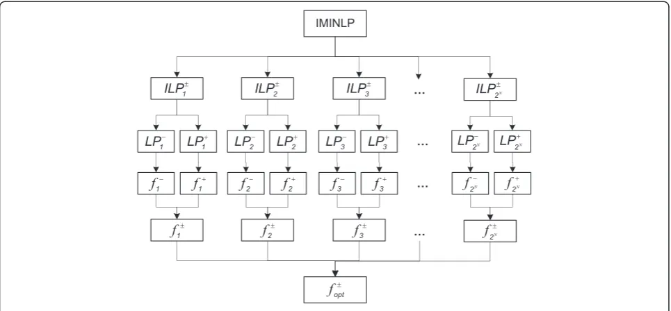
capture technology j should be applied to facility i, that means the total number of combinations of technology and facility is always limited in reality. Therefore, the IMINLP model can be converted into a number of ILP models by enumerating all possible values of Zij. Then,

Huang’s two-step method can be used to solve each ILP model separately. The final optimal solution must locate in the result set containing output of all ILP models, and it can be obtained according to corresponding criteria. Figure 2 illustrates the process of solving the IMINLP model.

In order to clearly address the general solution method, Model (2) can be rewritten as follows:

Minf ¼XN

i¼1e

i xi þ

XN

i¼1g

i xi yi ð3aÞ

subject to:

PN

i¼1ai xi ≥bi

PN

i¼1ci xi yi≥di

yi¼0 or1;8i

x_i ≥0;8i

8 > > < > >

: ð3bÞ

Define one combination of binary integer variableyas (y1, y2, . . ., yN), then the total number of combinations

foryis 2N. Therefore model (3) can be disassembled into 2N ILP models, and the jth ILP model can be expressed

as:

Minf_j¼XN

i¼1e

i xi þ

X

i2Qj

g_ix_i ð4aÞ

subject to:

PN

i¼1aixi ≥bi

P

i2Qjc

ixi ≥di

yi¼1;i2Qj

yi¼0;i2NQj

x_i ≥0 8i

8 > > > > < > > > > :

ð4bÞ

where Qj indicates the set of subscriptifor yi= 1, andj 2[1, 2N].

Obviously, such an ILP as model (4) can be tackled by being divided into two LP submodels f_j and f_jþ

(6)

is to minimize the cost, sof_j submodel should be firstly considered. It can be formulated as follows:

Minf_j¼XN

i¼1e

i xi þ

X

i2Qj

g_ix_i ð5aÞ

subject to:

PN

i¼1aixi ≥bi

P

i2Qjc

ixi ≥di

yi¼1; i2Qj

yi¼0; i2NQj

x_i ≥0;8i

8 > > > > < > > > > :

ð5bÞ

Let x_{ð Þ}_j_{i opt};yð Þji opt; and fj opt , and be the optimal

solu-tions off_jsubmodel. Then thef_jþ submodel can be for-mulated as:

Minf_jþ¼XN

i¼1e

þ

i xþi þ

XN

i¼1g

þ

i xþi yð Þji opt ð6aÞ

Subject to:

PN

i¼1aþixþi ≥bþi

PN

i¼1cþi xiþyð Þji opt≥diþ

xþ_i ≥x_{ð Þ}_j_{i opt};8i

8 > < >

: ð6bÞ

Assume the optimal solutions of f_jþ submodel were

xþ_{ð Þ}_j_{i opt};f_{j opt}þ . Thus, we have the solution for model (4):

f_{j opt} ¼ f_{j opt}− ;f_{j opt}þ

h i

;x_{ð Þ}_j_{i opt}¼ x_{ð Þ}−_j_{i opt};xþ_{ð Þ}_j_{i opt}

h i

;yð Þji opt ¼

1ði∈QiÞ;yð Þji opt¼0ði∈N−QiÞ. Accordingly, the other 2N

-1 solutions can be obtained by repeating the above pro-cedure. Define f_{j opt} is the median value of interval

f_{j opt} ¼ f_{j opt} ;f_{j opt}þ

h i

. Since the objective of model (3) is to find the minimum value of f, the screening rule for the optimal solution from result set can be summarized as that kth solution is the best solution if and only if

f_{k opt} ¼ min f₁_opt;f₂_opt;f₃_opt;. . .;f₂N_opt

.

As for the specific case of IMINLP expressed as model (2), there would be (J+ 1)K ILP models. In reality, CO2 capture technologies mainly include post-combustion, pre-combustion and oxyfuel combustion (Damen et al. 2006). That means J equals to 3, thus the total number of ILP models is 4K. The value ofKis also countable in a real regional electric power system. Hence the solution method discussed above is feasible in practice. Further-more, if there is enough information helpful for decision makers to eliminate impossible combinations of Zij, or

the decision makers only prefer several combinations ra-ther than all of them, the number of ILP models to be considered will decrease significantly. In other words, to solve such IMINLP model effectively, it is very

important to screen the essential scenarios beforehand based on decision makers’concerns. For example, if only the scenario that all facilities are employed post-combustion capture technology to reduce CO2emission needs to be considered, thus we have the corresponding combination ofZijas below:

Zij¼ 1 j¼1

0 j¼2;3 ;8i2½1;K

ð7Þ

where, j= 1 indicates post-combustion technology, and

j= 2,3 mean pre-combustion and oxyfuel combustion capture technologies, respectively. Correspondingly, the model (2) can be expressed as:

Minf¼PN_i_¼₁PT_t_¼₁CEG_itX_itþPN_i_¼₁P_tT_¼₁CCE_itY_it þPK

i¼1OiFi;j¼1CINi;j¼1;t¼1þ

PK

i¼1

PT

t¼1YitFi;j¼1CINi;j¼1;t

þPK

i¼1

PT

t¼1XitFi;j¼1COPi;j¼1;t

þPT

t¼1HtIMt

ð8aÞ

subject to:

XN

i¼1X

it þIMt ≥Dt ;8t ð8bÞ

Oiþ

XT

t¼1Y

it

U_it≥X_it;8i;t ð8cÞ

XN

i¼Kþ1X

it ≥NtDt ;8t ð8dÞ

X_itη_i 1Fi;j¼1λi;j¼1

1Fi;j¼1ri;j¼1

≤G_it;8i2½1;K;t

X_it≥0;8i;t ð8eÞ

0≤Y_it≤Emax_it;8i;t ð8gÞ

0≤IM_t≤E_tD_t ;8t ð8hÞ

This ILP model apparently can be solved through two-step method. The objective is to minimize system costs, therefore f_j submodel will be firstly considered. It can be formulated as:

Minf¼PN_i_¼₁PT_t_¼₁CEG_itX_itþPN_i_¼₁P_tT_¼₁CCE_itY_it þPK

i¼1OiFi;j¼1CINi;j¼1;t¼1þ

PK

i¼1

PT

t¼1YitFi;j¼1CINi;j¼1;t

þPK

i¼1

PT

t¼1XitFi;j¼1COPi;j¼1;t

þPT

t¼1HtIMt

ð9aÞ

subject to:

XN

i¼1X

(7)

Oiþ

XT

t¼1Y

it

U_it≥X_it;8i;t ð9cÞ

XN

i¼Kþ1X

it ≥NtDt ;8t ð9dÞ

X_itηþ_i 1Fi;j¼1λi;j¼1

1Fi;j¼1ri;j¼1

≤G_it;8i 2½1;K;t

ð10eÞ

X_it≥0;8i;t ð9fÞ

0≤Y_it≤Emax_it;8i;t ð9gÞ

0≤IM_t≤E_tD_t ;8t ð9hÞ

LetX_{it opt} ;Y_{it opt} ;IM_{t opt};f_opt be the optimal solutions of

f−submodel. Then thef+submodel can be formulated as: Minfþ¼PN_i_¼₁PT_t_¼₁CEGþ_itX_itþþPN_i_¼₁P_tT_¼₁CCEþ_itY_itþ þPK

i¼1OiFi;j¼1CINiþ;j¼1;t¼1þ

PK

i¼1

PT

t¼1YitþFi;j¼1CINiþ;j¼1;t

þPK

i¼1

PT

t¼1XitþFi;j¼1COPþi;j¼1;t

þPT

t¼1HtþIMþt

ð10aÞ

subject to:

XN

i¼1X

þ

it þIMþt ≥Dþt ;8t ð10bÞ

Oiþ

XT

t¼1Y

þ

it

U_itþ≥X_itþ;8i;t ð10cÞ

XN

i¼Kþ1X

þ

it ≥NtþDþt ;8t ð10dÞ

X_itþη_i 1Fi;j¼1λþi;j¼1

1Fi;j¼1riþ;j¼1

≤Gþ_it;8i 2½1;K;t

ð10eÞ

X_itþ≥X_{it opt} ;8i;t ð10fÞ

Y_{it opt} ≤Y_itþ≤Emaxþ_it;8i;t ð10gÞ

IM_{t opt}≤IM_tþ≤E_tþDþ_t ;8t ð10hÞ

Assume the optimal solutions of f+ submodel were

X_{it opt}þ ;Y_{it opt}þ ;IMþ_{t opt};f_optþ . Thus, we have the solution

for model (9) as follows: f_opt ¼ f_opt− ;f_optþ

h i

;X_{it opt} ¼

X_{it opt}− ;X_{it opt}þ

h i

;Y_{it opt} ¼

Y_{it opt}− ;Y_{it opt}þ

h i

;IM_{t opt}¼ IM_{t opt}− ;IM_{t opt}þ

h i

:

Case study

Overview of the study system

The regional electric power system to be studied is based on representative cost and technical data obtained from energy systems planning and CCS technologies related literatures (Lin and Huang 2009b; Li et al. 2010; Bowen 2011; Mitrovic and Malone 2011). The system covers a time horizon of three periods (t= 1,2,3), with each one having five years. Period 1 represents years 2012–2016, period 2 means 2017–2021, and period 3 would be 2022–2026, respectively. Its electricity gener-ation is supported by two coal-fired power plants (one is traditional with PC technology, the other has been built

Table 1 Existing capacities, allowable capacity expansion and generating efficiency for all facilities

Electricity generation facilities

Existing Capacity

Oi(GW)

Upper bounds of capacity expansionEmaxit(GW) Uit(PJ/GW)

t= 1 t= 2 t= 3 t= 1 t= 2 t= 3

PC (i = 1) 5.5 [1.5, 1.7] [1.2, 1.5] [1.0, 1.2] [90, 95] [95, 100] [100, 105]

NGCC (i = 2) 2.5 [0.9, 1.3] [0.8, 1.2] [1.0, 1.3] [80, 88] [85, 92] [90, 96]

IGCC (i = 3) 1.5 [2.0, 2.3] [2.5, 3.0] [3.0, 3.5] [95, 100] [100, 107] [105, 110]

Hydro power (i = 4) 0.5 [1.5, 1.8] [2.0, 2.5] [2.2, 2.6] [70, 75] [75, 80] [80, 85]

Wind power (i = 5) 0.2 [2.0, 2.5] [2.2, 2.8] [2.5, 3.0] [20, 24] [30, 34] [35, 38]

Table 2 Costs for electricity generation and capacity expansion

Cost of electricity generationCEGit($106_/PJ) _{Cost of capacity expansion}_CCEit_($106_/GW)

t= 1 t= 2 t= 3 t= 1 t= 2 t= 3

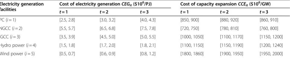
PC (i= 1) [2.5, 2.8] [3.0, 3.2] [4.0, 4.3] [850, 900] [880, 920] [860, 910]

NGCC (i= 2) [5.5, 5.7] [6.5, 6.8] [7.5, 7.8] [720, 750] [780, 810] [760, 800]

IGCC (i= 3) [3.5, 3.9] [4.5, 5.0] [5.0, 5.5] [1000, 1050] [1100, 1170] [1150, 1200]

Hydro power (i= 4) [1.5, 1.8] [1.7, 2.0] [1.8, 2.1] [1100, 1150] [1150, 1190] [1200, 1240]

(8)

recently with IGCC technology), one natural gas-fired power plant with NGCC technology, one hydro power station and one wind power plant. These five electricity facilities can be symbolized as i= 1,2,3,4,5 in sequence. Table 1 shows the existing capacity, allowable upper bound of capacity expansion and units of electricity pro-duction generated by per unit of capacity for each facil-ity. Table 2 lists the costs of electricity generation and capacity expansion. The CO2 capture technologies mainly contain post-combustion (j= 1), pre-combustion (j= 2), and oxyfuel combustion (j= 3). These three cap-ture technologies are only applicable to all fuel-fired fa-cilities. In particular, pre-combustion capture technology is not suitable for pulverised coal-fired power plants. Table 3 shows all parameters related to CCS technolo-gies. The total electricity demands would rise with the economic development. Thus the decision makers are forced to decide how to plan capacity expansion based on existing facilities to meet end-users’ increasing demands. Meanwhile, it is very important to apply suit-able and affordsuit-able CCS technologies to reduce CO2 emission. Electricity demandDtvaries for different periods

with [930, 1000] PJ in the 1st period, [1150, 1200] PJ in the 2nd period and [1330, 1400] PJ in the 3rd period. The re-newable energy rate Nt must meet the requirements of

[0.10, 0.12] for 1st period, [0.15, 0.18] for 2nd period and [0.20, 0.22] for 3rd period, respectively. Imported electricity priceHtshows an increase trend from [15, 18] $106/PJ to

[24, 30] $106/PJ, and ending with [40, 45] $106/PJ in the 3rd period. The imported rate for electricity Et is [0.08,

0.10] for 1st period, [0.09, 0.11] for 2nd period and [0.10, 0.12] for 3rd period, respectively.

The IMINLP model will be employed to facilitate plan-ning for this regional electric power system. The general so-lution method is to be used under two scenarios of CO2 emission limitation (i.e. high and low emission standards) in order to help planners well understand its impacts on the results (shown in Table 4). In reality, choosing suitable CO2capture technology for a given electricity facility is not only decided by technical feasibility, but also related to geo-graphical location availability for carbon transportation and storage, as well as its impacts on the social community and economic development. However, such information is us-ually not available or needs to be further investigated. Therefore, planners’preferences on CO2capture technolo-gies will be helpful and needs to be taken into consideration during the solving process. In this study, we assume that decision makers are only interested in three policies: (i) all facilities with post-combustion capture technologies; (ii) fa-cilities 1, 2 with post-combustion capture, facility 3 with pre-combustion; and (iii) all facilities with oxyfuel combus-tion technologies.

Result analysis

(1)Optimization solutions

Firstly, the results of planning without consideration of decision makers’interests in choosing CO2capture technologies are discussed. That means we need to cover all combination of technologies when disassembling the

Table 3 Parameters related to CCS technologies

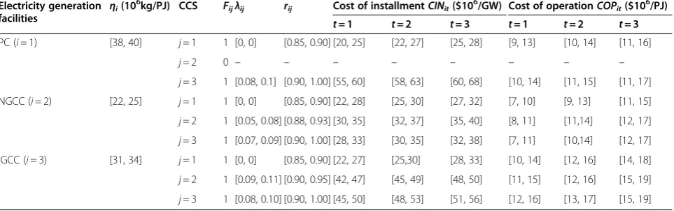
Electricity generation facilities ηi

(106kg/PJ) CCS Fijλij rij Cost of installmentCINit($106/GW) Cost of operationCOPit($106/PJ)

t= 1 t= 2 t= 3 t= 1 t= 2 t= 3

PC (_i= 1) [38, 40] _j= 1 1 [0, 0] [0.85, 0.90] [20, 25] [22, 27] [25, 28] [9, 13] [10, 14] [11, 16]

j= 2 0 _– _– _– _– _– _– _– _–

j= 3 1 [0.08, 0.1] [0.90, 1.00] [55, 60] [58, 63] [60, 68] [10, 14] [11, 15] [11, 17] NGCC (_i= 2) [22, 25] _j= 1 1 [0, 0] [0.85, 0.90] [22, 28] [25, 30] [27, 32] [7, 10] [9, 13] [11, 15]

j= 2 1 [0.05, 0.08] [0.88, 0.93] [30, 35] [32, 37] [35, 40] [8, 11] [11,14] [12, 17] j= 3 1 [0.07, 0.09] [0.90, 1.00] [28, 33] [30, 35] [32, 38] [7, 11] [10,14] [12, 17] IGCC (_i= 3) [31, 34] _j= 1 1 [0, 0] [0.85, 0.90] [22, 27] [25,30] [28, 33] [10, 14] [12, 16] [14, 18]

j= 2 1 [0.09, 0.11] [0.90, 0.95] [42, 47] [45, 49] [48, 50] [11, 15] [12, 16] [15, 19] j= 3 1 [0.08, 0.10] [0.90, 1.00] [45, 50] [48, 53] [51, 56] [12, 16] [13, 17] [15, 19] “–”indicates not applicable.

Table 4 Limitations on CO2emission for two scenarios

High emission scenarioGit(106_kg) _{Low emission scenario}_G it(106_kg)

t= 1 t= 2 t= 3 t= 1 t= 2 t= 3

PC (i= 1) [3000, 3150] [2800,3000] [2500, 2650] [1600, 1650] [1300, 1350] [1150, 1230]

NGCC (i= 2) [1800, 1900] [1700, 1800] [1600, 1700] [800, 860] [760, 800] [720, 780]

(9)

IMINLP model into (J+ 1)KILP models. The optimal solutions for two CO2emission scenarios concerning imported electricity, generation of local facilities and their corresponding capacity expansion in periods 1, 2, and 3 are listed in Table5. The total cost for high emission scenario is [53714.63, 69399.39]$106, which is obviously lower than the cost at low emission scenario about [65326.26, 81953.3]$106. In order to make better

understanding of the results, some comparisons based on these two scenarios are further conducted. Figure3 shows the comparison of electricity supply schemes between high and low CO2emission scenarios. There are apparent differences in the trends of energy supply from import for facility 1 and 3. In the high emission scenario, contributions of imported sector and facility 3 are decreasing within the range below 100 PJ, while electricity generated by facility 1 is increasing from approximate 500 to 650 PJ. By contrast, the low emission scenario indicates another situation in the opposite way regarding the electricity supplied by imports for facility 1 and 3. The electricity contribution of imports and facility 3 are always growing within the whole planning horizon, especially, generation of facility 3 has jumped from about 50 to 300 PJ. Meanwhile, facility 1 shows a descending

way from 400 to 300 PJ. This comparison reveals that facilities 1 and 3 are playing important role in the total CO2emission of the study power system as there are significant difference between high and low emission scenarios. As for the other three facilities (2, 4, and 5), there are no obvious differences in the comparison. In other words, it can be seen that the contributions of these facilities in some extent have relative smaller or no impacts on the CO2emission. In fact, the facilities 4 and 5 indicate hydro and wind power plants, and facility 2 means natural gas-fired power plant. Hydro and wind power indeed have no CO2 emission except the natural gas power, however, its impact stands less than that of coal-fired plants (i.e. facilities 1 and 3). The electricity is then imported to cover the shortage while capacity expansion can not meet the increasing demands under restricted CO2emission standards. The comparison of capacity expansion for two scenarios is presented in Figure4. The expansions for hydro and wind power are almost keeping a stable level. But for the facilities 1, 2, and 3, the capacity expansions are very different. In particular, the expanding scale of facility 1 stands at the highest among these three facilities in the high emission scenario; however, its expansion is not suggested at all in the low emission scenario. The reason is obviously

Table 5 Optimal solutions under two CO2emission scenarios

Facility High emission scenario Low emission scenario

t= 1 t= 2 t= 3 t= 1 t= 2 t= 3

IMt(PJ) [68.47, 68.47] [39.85, 39.85] [40.18, 40.18] [74.40, 74.40] [103.50, 103.50] [133.00, 133.00] Xit(PJ) i= 1 [495.00, 507.66] [636.50, 636.50] [650.00, 657.68] [434.78, 471.05] [353.26, 353.26] [312.50, 329.18] i= 2 [200.00, 220.00] [212.50, 212.50] [315.00, 315.00] [229.32, 252.25] [280.50, 280.50] [309.68, 309.68] i= 3 [73.50, 83.87] [67.60, 80.65] [58.80, 69.35] [47.50, 47.50] [219.24, 219.24] [290.89, 290.89] i= 4 [89.00, 115.20] [187.50, 223.70] [216.00, 263.50] [140.00, 150.00] [187.50, 236.70] [216.00, 263.50] i= 5 [4.00, 4.80] [6.00, 6.80] [50.00, 54.29] [4.00, 4.80] [6.00, 6.80] [67.94, 73.76] Yit(GW) i= 1 [0.00, 0.00] [1.20, 1.20] [1.00, 1.00] [0.00, 0.00] [0.00, 0.00] [0.00, 0.00]

i= 2 [0.00, 0.00] [0.00, 0.00] [1.00, 1.00] [0.37, 0.37] [0.80, 0.80] [0.94, 0.94] i= 3 [0.27, 0.34] [0.18, 0.25] [0.06, 0.13] [0.00, 0.00] [1.69, 1.69] [2.27, 2.27] i= 4 [0.78, 1.04] [2.00, 2.30] [2.20, 2.60] [1.50, 1.50] [2.00, 2.46] [2.20, 2.60] i= 5 [0.00, 0.00] [0.00, 0.00] [1.23, 1.23] [0.00, 0.00] [0.00, 0.00] [1.74, 1.74] f($106₎ _{[53714.63, 69399.39]} _{[65326.26, 81953.30]}

0 100 200 300 400 500 600 700

Imported Facility 1 Facility 2 Facility 3 Facility 4 Facility 5 2012-2016 2017-2021 2022-2026 Upper bound

0 100 200 300 400 500 600 700

Imported Facility 1 Facility 2 Facility 3 Facility 4 Facility 5

(a)

E

le

c

tr

ic

it

y s

u

p

ly

(P

J)

E

le

c

tr

ic

it

y s

u

p

ly

(P

J)

(b)

(10)

related to its important contribution to the total CO2 emission of the entire electric power system.

Secondly, the rates of imported electricity and renewable energy in the two emission scenarios are compared to further assess the security of power system structure. The results are shown in Figure5. The rate of imported electricity is increasing to about 8% in the low emission scenario; the reason is that capacity expansion of local facilities is restricted by the low emission standards. Therefore, electricity needs to be imported to meet the growing demands. The declining trend of imported electricity in high emission scenario also demonstrates its interaction in the opposite way. Obviously, the higher the rate of imported electricity, the more insecurity or instability the power supply structure will be. In turn, the lower the rate, the more CO2will be emitted. Therefore, there is a tradeoff between the safety of power supply framework and lower CO2emission. As shown in Figure5, there is no significant change in the rate of renewable energy in two scenarios. Such relative stability is mainly limited by the corresponding

constraints in the IMINLP. (2)Policy analysis

Decision makers’preference plays an important role in the selection and penetration of CO2capture and storage technologies; furthermore, it could affect the structure of electricity supply and capacity expansion planning in the regional electric power system. Therefore, three scenarios are conducted to demonstrate the influences of different policies for CO2sequestration. Policy on all facilities being

applied post-combustion capture technologies is considered in scenario A; facilities 1, 2 with post-combustion capture, facility 3 with pre-combustion is considered in scenario B; and all facilities with oxyfuel combustion technologies is processed in scenario C. The total system costs for three scenarios are [58232.08, 74128.19] $106, [57777.78, 73682.44] $106, and [56265.91, 73380.01] $106respectively. The electricity supplies under different scenarios during the planning period are shown in Figure6. There is no

difference in the structure of electricity supply between scenarios A and B. The results for capacity expansion are also the same. The reason should be the only difference in choosing CO2sequestration technologies for facility 3. However, the system costs for scenario A and B are entirely different. This indicates the oxyfuel combustion is a cheaper way for facility 3 compared with post-combustion

technology. Under scenario C, the electricity supply changes a lot by enhancing coal-fired power during the whole planning period, while scenarios A and B are both showing decreasing trends. Another apparent difference lies on the facility 3 with NGCC conversion technology, which plays an important role on the electricity supply under scenarios A and B in period 3. In contrast, its contribution in scenario C shows considerable decline, and electricity supplied by facility 1 is correspondingly increased to meet the end users’ demands. Meanwhile, the results for capacity expansion of facility 1 and 3 under three scenarios are changing

according to their proportions in the total electricity supply. For example, there is no need to expand the capacity of facility 1 for both scenario A and B during the planning 0 0.5 1 1.5 2 2.5 3 3.5 4 4.5 5 5.5 6

Facility 1 Facility 2 Facility 3 Facility 4 Facility 5

E lect ri c gener a ti on capaci ty ( G W ) 0 0.5 1 1.5 2 2.5 3 3.5 4 4.5 5 5.5 6

Facility 1 Facility 2 Facility 3 Facility 4 Facility 5

E lect ri c gener a ti on capaci ty ( G W

) Existing capacity Capacity expansion (2012-2016)

Capacity expansion (2017-2021) Capacity expansion (2022-2026) Upper bound of expansion

(a) (b)

Figure 4Comparison of electric generation capacity expansion in two scenarios: (a) results of high emission scenario; (b) results of

low emission scenario.

0 2 4 6 8 10 12

2012-2016 2017-2021 2022-2026

Time period

R

a

te of i

m por ted el ec tr ic it y ( % )

Upper bound Low er bound

High emission scenario Low emission scenario

0 5 10 15 20 25 30

2012-2016 2017-2021 2022-2026

Time period R a te of r e new abl e ener gy ( % )

Upper bound Low er bound

High emission scenario Low emission scenario

(a) (b)

Figure 5Comparison between of the rate of imported electricity for two CO2 emission scenarios: (a) rate of imported electricity; (b)

(11)

horizon, but under scenario C, its capacity can not satisfy the necessary supply any more. Consequently, the expansion options of [1.2, 1.2] GW and [1.0, 1.0] GW should be taken in the period 2 and 3 for facility 1 at scenario C. There is no apparent discrepancy in electricity supply of facility 2, 4 and 5 for three scenarios, so is the capacity expansion. As for the imported electricity, it holds a noticeable position in the whole electricity supply in period 1 and 2 for all scenarios; however, it decreases to zero in period 3, which means the shortage of electricity can be handled through capacity expansion.

The above analysis could generate alternative decision bases for planners regarding CO2sequestration

technologies. For example, scenario C with the least cost may be preferred in recessionary period; however, this cost-efficient strategy should be based on sufficient coal supply. If there are more oil and gas reserved in this region, scenarios A and B should be considered. Although these two scenarios generate the same schemes for both electricity supply and capacity expansion, scenario B is more efficient in the total system cost than scenario C. Therefore, scenario B would be preferred.

0 200 400 600 800 1000 1200 1400 1600

t=1 (lower bound) t=1 (upper bound) t=2 (lower bound) t=2 (upper bound) t=3 (lower bound) t=3 (upper bound)

Electricity supply (PJ)

Imported Facility 1 Facility 2 Facility 3 Facility 4 Facility 5

0 200 400 600 800 1000 1200 1400 1600

(a)

(b)

(c)

(12)

Conclusions

An interval mixed-integer non-linear programming (IMINLP) model was developed in this study to assist re-gional electric power systems planning under uncertainty. CO2capture and storage technologies had been introduced to the IMINLP model to help reduce carbon emission. The developed IMINLP model could be disassembled into a number of ILP models, then two-step method (TSM) was used to obtain the optimal solutions. A case study was pro-vided for demonstrating applicability of the developed method. The results indicated that the IMINLP was effect-ive in providing alternateffect-ive decision bases for electricity planning under uncertainty.

This study is the first attempt for planning regional elec-tric power systems with consideration of CO2capture and storage technologies. The solution method for the IMINLP model is effective only if the total number of disassembled ILP models could be finite. As for the complicated regional electric power systems, if there are a large number of facilities to be planned with CO2sequestration technolo-gies, this method would be computation-consuming. In addition, we assume that the cost of power plant expan-sion would be independent to the capacity of expanexpan-sion. That means the economies of scale issue is not considered in the IMINLP model. In fact, this issue may exist in some real world problems which will lead to a linear or more complicated relationship between the cost of power plant expansion and the capacity of expansion. In that case, the developed model is not applicable any more. Therefore, further studies are desired to tackle this issue and make the IMINLP model more applicable in the real world.

Competing interests

The authors declare that they have no competing interests.

Acknowledgements

This research was supported by the Program for Innovative Research Team (IRT1127), the MOE Key Project Program (311013), the Natural Science and Engineering Research Council of Canada, and the Major Project Program of the Natural Sciences Foundation (51190095).

Author details 1

Institute for Energy, Environment and Sustainable Communities, University of Regina, Regina, Saskatchewan, Canada S4S 0A2.2_{Institute for Energy,} Environment and Sustainability Research, UR-NCEPU, North China Electric Power University, Beijing 102206, China.3_{MOE Key Laboratory of Regional} Energy and Environmental Systems Optimization, Resources and Environmental Research Academy, North China Electric Power University, Beijing 102206, China.

Authors’contributions

The work presented here was carried out in collaboration between all authors. Dr. G. H. Huang and Dr. Q. G. Lin defined the research theme. Mr. X. Q. Wang developed the IMINLP model and the solution method based on

Dr. G. H. Huang’s previous works, carried out the case study, analyzed the

data, interpreted the results and wrote the paper. All authors have contributed to, seen and approved the manuscript.

Received: 4 April 2012 Accepted: 14 August 2012 Published: 14 August 2012

References

Bowen F (2011) Carbon capture and storage as a corporate technology strategy

challenge. Energy Policy 39:2256–2264

Cai YP, Huang GH, Lin QG, Nie XH, Tan Q (2009a) An optimization-model-based interactive decision support system for regional energy management

systems planning under uncertainty. Expert Syst Appl 36:3470–3482

Cai YP, Huang GH, Yang ZF (2009b) Identification of optimal strategies for energy management systems planning under multiple uncertainties. Appl Energy 86:480–495

Cao MF, Huang GH (2011) Scenario-based methods for interval linear

programming problems. J Environ Inform 17:65–74

Cao MF, Huang GH, Lin QG (2010) Integer programming with random-boundary

intervals for planning municipal power systems. Appl Energy 87:2506–2516

Damen K, van Troost M, Faaij A, Turkenburg W (2006) A comparison of electricity and hydrogen production systems with co2 capture and storage. Part a: Review and selection of promising conversion and capture technologies.

Prog Energy Combust Sci 32:215–246

de Coninck H, Stephens JC, Metz B (2009) Global learning on carbon capture and storage: A call for strong international cooperation on ccs demonstration.

Energy Policy 37:2161–2165

de Lucena AFP, Schaeffer R, Szklo AS (2010) Least-cost adaptation options for global climate change impacts on the brazilian electric power system. Glob

Environ Chang 20:342–350

Fan YR, Huang GH (2012) A robust two-step method for solving interval linear programming problems within an environmental management context. J

Environ Inform 19:1–12

Hidy GM, Spencer DF (1994) Climate alteration a global issue for the electric

power industry in the 21st century. Energy Policy 22:1005–1027

Huang GH, Baetz BW, Patry GG (1992) A grey linear programming appoach for municipal solid waste management planning under uncertainty. Civ Eng Syst 9:319–335

Huang GH, Baetz BW, Patry GG (1995a) Grey fuzzy integer programming: An application to regional waste management planning under uncertainty.

Socio Econ Plan Sci 29:17–38

Huang GH, Baetz BW, Patry GG (1995b) Grey integer programming: An application to waste management planning under uncertainty. Eur J Oper Res 83:594–620

Huang GH, Cao MF (2011) Analysis of solution methods for interval linear

programming. J Environ Inform 17:54–64

Karaki SH, Chaaban FB, Al-Nakhl N, Tarhini KA (2002) Power generation expansion planning with environmental consideration for lebanon. Int J Electr Power

Energy Syst 24:611–619

Li YF, Huang GH, Li YP, Xu Y, Chen WT (2010) Regional-scale electric power

system planning under uncertainty–a multistage interval-stochastic integer

linear programming approach. Energy Policy 38:475–490

Lin QG, Huang GH (2009a) A dynamic inexact energy systems planning model for supporting greenhouse-gas emission management and sustainable

renewable energy development under uncertainty–a case study for the city

of waterloo, canada. Renew Sust Energ Rev 13:1836–1853

Lin QG, Huang GH (2009b) Planning of energy system management and

ghg-emission control in the municipality of beijing–an inexact-dynamic stochastic

programming model. Energy Policy 37:4463–4473

Lin QG, Huang GH (2010) An inexact two-stage stochastic energy systems planning model for managing greenhouse gas emission at a municipal level.

Energy 35:2270–2280

Lin QG, Huang GH, Bass B, Nie XH, Zhang XD, Qin XS (2010) Emdss: An optimization-based decision support system for energy systems management under changing climate conditions - an application to the

toronto-niagara region, canada. Expert Syst Appl 37:5040–5051

Merrill HM, Wood AJ (1991) Risk and uncertainty in power system planning. Int J

Electr Power Energy Syst 13:81–90

Mitrovic M, Malone A (2011) Carbon capture and storage (ccs) demonstration

projects in canada. Energy Procedia 4:5685–5691

Sanghvi AP, Shavel IH (1984) Incorporating explicit loss-of-load probability constraints in mathematical programming models for power system capacity

planning. Int J Electr Power Energy Syst 6:239–247

Voropai NI, Ivanova EY (2002) Multi-criteria decision analysis techniques in electric power system expansion planning. Int J Electr Power Energy Syst 24:71–78

(13)

storage across electric power regions in the united states. Int J Greenh Gas Control 1:261–270

Wu NN, Yan XP, Huang GH, Wu CZ, Gong J (2010) Urban environment-oriented

traffic zoning based on spatial cluster analysis. J Environ Inform 15:111–119

Yan XP, Ma XF, Huang GH, Wu CZ (2010) An inexact transportation planning model for supporting vehicle emissions management. J Environ Inform 15:87–98

Zafer Yakin M, McFarland JW (1987) Electric generating capacity planning: A

nonlinear programming approach. Electr Power Syst Res 12:1–9

doi:10.1186/2193-2697-1-1

Cite this article as:Wanget al.:An interval mixed-integer non-linear programming model to support regional electric power systems

planning with CO2capture and storage under uncertainty.Environmental

Systems Research20121:1.