An impossibility theorem for Parameter
Independent hidden variable theories
Gijs Leegwater
∗March 31, 2016
Abstract
Recently, Roger Colbeck and Renato Renner (C&R) have claimed that ‘[n]o extension of quantum theory can have improved predictive power’ (Colbeck & Renner, 2011, 2012b). If correct, this is a spectacular impos-sibility theorem for hidden variable theories, which is more general than the theorems of Bell (1964) and Leggett (2003). Also, C&R have used their claim in attempt to prove that a system’s quantum-mechanical wave function is in a one-to-one correspondence with its ‘ontic’ state (Colbeck & Renner, 2012a). C&R’s claim essentially means that in any hidden variable theory that is compatible with quantum-mechanical predictions, probabilities of measurement outcomes are independent of these hidden variables. This makes such variables otiose. On closer inspection, how-ever, the generality and validity of the claim can be contested. First, it is based on an assumption called ‘Freedom of Choice’. As the name suggests, this assumption involves the independence of an experimenter’s choice of measurement settings. But in the way C&R define this as-sumption, a no-signalling condition is surreptitiously presupposed, mak-ing the assumption less innocent than it sounds. When usmak-ing this defini-tion, any hidden variable theory violating Parameter Independence, such as Bohmian Mechanics, is immediately shown to be incompatible with quantum-mechanical predictions. Also, the argument of C&R is hard to follow and their mathematical derivation contains several gaps, some of which cannot be closed in the way they suggest. We shall show that these gaps can be filled. The issue with the ‘Freedom of Choice’ assump-tion can be circumvented by explicitly assuming Parameter Independence. This makes the result less general, but better founded. We then obtain an impossibility theorem for hidden variable theories satisfying Parame-ter Independence only. As stated above, such hidden variable theories are impossible in the sense that any supplemental variables have no bearing on outcome probabilities, and are therefore trivial. So, while quantum mechanics itself satisfies Parameter Independence, if a variable is added that changes the outcome probabilities, however slightly, Parameter Inde-pendence must be violated.
∗Erasmus University Rotterdam, Faculty of Philosophy, Burg. Oudlaan 50, 3062 PA Rot-terdam, The Netherlands. E-mail: [email protected]
1 INTRODUCTION 2
1
Introduction
In 1935, Einstein, Podolsky and Rosen famously argued that quantum mechan-ics is incomplete and that there might be another theory that does provide a complete description of physical reality (Einstein et al., 1935). One class of candidates for such a theory is the class of so-called ‘hidden variable theories’, which supplement the quantum state with extra variables.1 Hidden variable theories have indeed been developed, for example the de Broglie–Bohm theory (Bohm, 1952), which is deterministic and complete in Einstein’s sense. However, a number of impossibility theorems have been derived, showing that large classes of possible hidden variable theories are incompatible with quantum-mechanical predictions. John Bell proved such incompatibility for local deterministic hid-den variable theories (Bell, 1964), as well as for local stochastic hidhid-den variable theories (Bell, 2004), while the incompatibility of ‘crypto-nonlocal’ theories was proven by Leggett (2003). Still, a large class of hidden variable theories, like the de Broglie–Bohm theory, remains unscathed by these impossibility theorems.
The hidden variable theories shown to be incompatible by Bell are theories satisfying a criterion called Factorizability (Fine, 1982), which is equivalent to the conjunction of two locality conditions coined by Abner Shimony (1984): Pa-rameter Independence (ParInd) and Outcome Independence (OutInd). There-fore, any hidden variable theory compatible with quantum mechanics violates at least one of these two conditions. In this article we claim something stronger: any hidden variable theory compatible with quantum mechanics violates ParInd, except for ‘trivial’ hidden variable theories, where the values of the hidden vari-ables have no bearing on measurement outcome probabilities.
This article is based on recent work by Roger Colbeck and Renato Renner (C&R), who have claimed that they have derived an even more general impos-sibility theorem (Colbeck & Renner, 2011, 2012b). Stating that ‘[n]o extension of quantum theory can have improved predictive power’, they essentially claim thatanynon-trivial hidden variable theory, also if it violates ParInd (like the de Broglie–Bohm theory), is incompatible with quantum-mechanical predictions. Given the wide scope of this claim, this would be a spectacular result, which would to a great extent put constraints on any possible future theory replacing quantum mechanics.
However, C&R’s claim crucially hinges on an assumption dubbed ‘Freedom of Choice’. As the name suggests, this assumption is meant to be about the freedom of experimenters to choose their measurement settings. From this as-sumption, C&R derive ‘no-signalling’, which is essentially equal to ParInd. Nev-ertheless, when inspecting the way ‘Freedom of Choice’ is defined, it becomes apparent that ParInd is in fact part of this assumption. Most criticism of C&R’s work focuses on this issue (Ghirardi & Romano, 2013a,b; Colbeck & Renner, 2013; Leifer, 2014; Landsman, 2015). We agree with the criticism: C&R’s ‘Free-dom of Choice’ assumption is much stronger than its name suggests. Therefore, while the impression is given that any hidden variable theory with free exper-imenters is shown to be incompatible with QM, in fact their result applies to a smaller class of hidden variable theories: those satisfying ParInd. The de Broglie–Bohm theory, which violates ParInd, is therefore not shown to be
in-1In the literature, sometimes the term ‘hidden variable theory’ is understood to refer only
1 INTRODUCTION 3
compatible after all.
If the above issue was the only problem with C&R’s work, the result of the present article could easily be achieved by adding ParInd as an explicit assump-tion. The theorem would then still be an interesting impossibility theorem, being more general than the theorems of Bell and Leggett. However, there are more shortcomings in the work of C&R. First, it is hard to understand, even for experts. Valerio Scarani (2013) says:
‘Beyond the case of the maximally entangled state, which had been settled in a previous paper, they prove something that I honestly have not fully understood. Indeed, so many other colleagues have misunderstood this work, that the authors prepared a page of FAQs [(Colbeck, 2010)] (extremely rare for a scientific paper) and a later, clearer version [(Colbeck & Renner, 2012b)].’
The case of the maximally entangled state that Scarani refers to corresponds to the triviality claim of C&R restricted to local measurements on a Bell state. This result consists of the statement that not only the quantum-mechanical outcome probabilities, but also the outcome probabilities in any hidden vari-able theory equal 1/2 (in the present paper, this result is presented in Section 4). Some authors, for example Antonio Di Lorenzo (2012), appear to have un-derstood C&R as deriving only this result, which, as Scarani alludes to, had been derived before. Actually, for C&R this is only the first step in proving the more general theorem that probabilities in hidden variable theories are always equal to the quantum-mechanical probabilities.
More importantly, C&R’s derivation contains gaps, of which some are al-legedly filled in other publications, while others remain. One example is their careless handling of limits: in more than one occasion results are derived that only hold approximately, which are then used as if they hold exactly.2
Because of these shortcomings, at present no acceptable deduction of the impossibility theorem for hidden variable theories satisfying ParInd exists in the literature. In this article we attempt to repair the shortcomings of C&R’s derivation in order to establish such a deduction. A step that is not explicitly mentioned by C&R, involving the relation between measurements on entangled states and measurements on non-entangled states, is formulated explicitly. Fur-thermore, we give a deduction that is mathematically acceptable. We emphasize that this does not consist of simply filling some gaps. For some parts of the de-duction to succeed, an entirely new strategy has to be constructed, or so we claim. This is especially the case when taking proper care of all the limits used in the proof. Also, some parts of the deduction can, in our opinion, be consid-erably simplified, especially the first steps. For these reasons, in this article we do not merely point out all the shortcomings in the original derivation; rather, we construct a new version of it.
C&R have also used their claim in an attempt to answer the question whether the quantum-mechanical wave function is ‘ontic’ or ‘epistemic’. Since the ap-pearance of the Pusey-Barret-Rudulph (PBR) theorem (Pusey et al., 2012), this is a hotly debated topic. On the basis of their claim, C&R argue not only that the wave function is ontic, but also that it is in a one-to-one correspondence with its ontic state (Colbeck & Renner, 2012a). In the Discussion (Section 9), we
2 NOTATION 4
shall consider what remains of thisψ-ontology result if C&R’s claim is replaced by the weaker result deduced in this article.
The result will be deduced in several steps. The first steps are quite simple and correspond to results that existed already before the work of C&R. How-ever, we believe that even for those whom are already familiar with this result, these steps are still of value since they are considerably simplified, only using a triangle inequality and a simple inequality from probability theory. The fi-nal steps require more mathematics and may be harder to follow. Most of the mathematics is relegated to appendices, so as not to distract the reader from the central line of reasoning. If the reader want to shorten the reading time, the best section to skip might be Section 7, because the extent of the general-ization (from states with coefficients that are square roots of rational numbers to any coefficients) is relatively small compared to the amount of mathematics needed. It is however a necessary part for deriving the full theoretical result. In the Discussion, I shall mention the most important differences between our deduction and that of C&R.
2
Notation
Quantum-mechanical systems are referred to by the symbols A, B, A0, B0 etc.
To denote composite systems, the symbols for the subsystems are combined, for exampleAB andAA0A00. The Hilbert space of systemA is denoted byHA, a
state as |ψiA and an operator on HA as UA. For notational convenience, the
subscript attached to a state may be omitted when no confusion is possible, especially when large composite systems likeAA0A00BB0B00 are involved. The symbol⊗for taking tensor products is also often omitted, and we freely change the order of states when combining systems, so that we can write
UAB(|iiA⊗ |jiB)≡UAB(|jiB⊗ |iiA)≡UAB(|jiB|iiA). (2.1)
We also write [ψ]A := |ψi
AAhψ|, and Nr for the set {0,1, . . . , r−1}. The
cardinality of a setJ is written as #J, and sequences are notated as (xn)10n=0.
In this article, mainly projective measurements with a finite number of out-comes are considered. Such measurements are defined by a complete set of orthogonal projectors{EˆA
i } d−1
i=0 withd∈N, each projector corresponding to a
possible outcome. If all projectors are 1-dimensional, the set of projectors can be written as{[i]A}di=0−1, in which case it is said that the measurement is performed ‘in the basis {|iiA}di=0−1’. We also allow ourselves to say this when {|iiA}di=0−1
is not a basis of HA, but of a strict subspace of HA. In this case the
corre-sponding complete set of orthogonal projectors is{[i]A}di=0−1∪ {IA−Pdi=0−1[i]
A}.
Equivalently, a projective measurement can be characterized by an observable (a Hermitian operator) of which the eigenspaces corresponding to the eigen-values equal the ranges of the projectors{EˆA
i } d−1
i=0. Two observables which are
equal up to their eigenvalues represent the same measurement. So, if a measure-ment is characterized by the complete set of orthogonal projectors{EˆA
i } d−1
i=0, a
corresponding observable is
ˆ
OA=
d−1 X
i=0
2 NOTATION 5
where the ei ∈R are (distinct) eigenvalues. Probabilities of outcomes can be expressed using the projectors:
Pr|ψiAEˆA
i
=hψ|AEˆiA|ψiA. (2.3)
The superscript including the state of the system may be omitted if no confusion is possible. Also, sometimes the superscript on the observable is omitted, for example when a general form of an observable is defined which can be applied to multiple systems.
Often measurements are considered on subsystems, and the pure state of the composite system is specified:
Pr|φiABEˆA
i
. (2.4)
To express probabilities using observables, we associate to any observable ˆ
OA a random variable OA. We want to emphasize that we only consider joint distributions of random variables if their associated observables are jointly mea-surable (and therefore commute). It is well known that if one defines joint distributions for non-commuting observables, then the corresponding random variables are subject to additional constraints, in the form of a Bell inequality (Fine, 1982), which we want to avoid. With this in place, probabilities can be expressed using the random variables associated with observables:
Pr OA=ei
= PrEˆiA. (2.5)
We will see in the next section that the hidden variable theories we consider lead to a decomposition of the quantum probabilities. That is, an extra variableλis added to each quantum probability, and there is a measureµ(λ) such that, when averaging overλusing this measure, the quantum probability is retrieved. The probabilities in hidden variable theories and in a decomposition are called λ -probabilities. In decompositions, these probabilities are denoted as the quantum probabilities, withλadded as a subscript:
Prλ OA=ei
= Prλ
ˆ
EiA
ˆ
OA. (2.6)
In the notation using projectors, we have added an extra subscript indicating the measured observable. This is because a λ-probability might be contextual, depending not only on the projector ˆEA
i , but also on the other projectors
char-acterizing the measurement.3
Identities involvingλ-probabilities appearing in this article mostly hold ‘al-most everywhere’, i.e. for all λ in a subset Ω⊂Λ with µ(Ω) = 1, where µ is a measure on the measurable space Λ. Wherever this is the case, the symbol
.
= is used. Often we will consider λ-probabilities, expressed using a projector, that are almost everywhere independent of the observable that is measured. For example, we might have4
∀OˆA: Prλ
ˆ
EiA
ˆ
OA
.
= 1
2. (2.7)
3Note that this is a specific type of contextuality which is, for example, different from the
contextuality considered in the Kochen–Specken Theorem (Kochen & Specker, 1975), which concerns a dependence ofvalues, instead of probabilities, on the measurement context.
4The quantifier in (2.7) ranges over all observables that include ˆEA
i in their sets of
3 THEOREM 6
In such cases, we allow ourselves to drop the observable from the notation, so the above can be rewritten as
Prλ
ˆ
EiA=. 1
2, (2.8)
although Prλ
ˆ
EA i
might not be well-defined for a measure zero subset of λ’s. A λ-probability is called trivial if it equals the corresponding quantum-mechanical probability for almost every λ. A decomposition is called trivial if all the λ-probabilities occurring in it are trivial. Also, a hidden variable theory is called trivial if all theλ-probabilities occurring in it are trivial.
From Section 6 onwards, limits are taken involving multiple variables. These are alwaysrepeated limits. If, for example, we write
lim
l→∞nlim→∞f(n, l) = liml→∞
lim
n→∞f(n, l)
, (2.9)
this means that first the limitn→ ∞is taken, and limn→∞f(n, l) exists. Note
that the order of the limits is important: it might be that in the above case liml→∞f(n, l) does not exist in which case limn→∞liml→∞f(n, l) is not
well-defined. If > 0 and liml→∞limn→∞f(n, l) = 0 then, to find ann and an l
such that |f(n, l)|< , first anl large enough must be chosen, and then an n
large enough.
3
Theorem
The main result of this article concernsλ-probabilities for measurements on a systemAin the state|ψiA, to which a hidden variable theory assigns an extra
variableλ. Thisλis distributed according to some measureµ(λ), which might depend not only on the quantum state|ψiA but also on other factors, like the
specific method that was used to prepare the state. Now, given a value ofλ, the outcome probabilities of a measurement of system Ain the state|ψiA may
dif-fer from the quantum-mechanical probabilities. Also, the λ-probabilities might have additional dependencies compared with quantum probabilities. For exam-ple, λ-probabilities may be contextual, as mentioned in the previous section. They may also depend on the specific implementation of the measurement. If a
λ-probability for a certain implementation of the measurement were non-trivial, this would generate a non-trivial decomposition. Therefore, it is enough to show that there is no non-trivial decomposition, and additional factors such as the specific implementation of the measurement do not have to be included when writing downλ-probabilities: Pr|ψiA
λ
ˆ
EA i
ˆ
OA.
5
Now, given a value ofλnot only the outcome probabilities of a measurement of system A in the state |ψiA may differ, but also outcome probabilities of
5More specifically, factors such as the specific implementation can be omitted because
3 THEOREM 7
measurements on systems which have interacted with A. For example, Amay be coupled to a system B in the following way:
|ψiA|0iB 7→ d−1 X
j=0
ˆ
EjA|ψiA|jiB (3.10)
where {EˆjA}jd=0−1 is a complete set of orthogonal projectors and{|jiB}dj−=01 a set
of orthonormal vectors. Then, a measurement in the basis{|jiB}dj−=01 onB can
be considered, and for this measurement the λ-probabilities might also differ from the quantum-mechanical probabilities. Like above, there might be addi-tional dependencies, such as on the specific implementation of the interaction betweenAandB. Again, a non-trivialλ-probability would imply a non-trivial decomposition, and therefore these additional dependencies can be omitted, so we write down the λ-probability as
Pr|φiAB
λ [i] B
ˆ
OB. (3.11)
So, here λstill refers to the variable assigned to system A when it was in the state|ψiA. We will also consider measurements on more complicated
compos-ite systems like AA0A00BB0B00, and also in these cases, λalways refers to the original systemA, and there is only one measureµ(λ) that is considered.
We can now further impose conditions on such decompositions. For ex-ample, we might imposenon-contextuality, meaning that theλ-probability of a measurement outcome only depends on the corresponding projector, and not on the other projectors characterizing the measurement. This is however a strong condition, as it follows from Gleason’s theorem that such decompositions are trivial if the dimension of the Hilbert space of the system is at least 3.6 We will,
however, impose the following conditions:
• CompQuant: Compatibility with Quantum-Mechanical Predic-tions
We consider theories where the quantum state|ψiAis supplemented with
a hidden variable λ, which assumes a value from the measurable space Λ. It is assumed that the quantum-mechanical probabilities are retrieved when averaging using the measure µ(λ). This means that, for any de-composition generated by the hidden variable theory, for every projective measurement involving state|φi, observable ˆO and projector ˆE,
Z
Λ
dµ(λ)Pr|λφiEˆ
ˆ
O = Pr
|φiEˆ=hφ|E|φi.ˆ (3.12)
6According to Gleason’s theorem (Gleason, 1957), for any Hilbert space with dimension
at least 3, any probability measure over the projectors corresponds to a unique density matrix ρsatisfying Pr
ˆ E
= Tr
ρEˆ
for all projectors ˆE. Now, if Pr
ˆ E
could be
de-composed so that Pr
ˆ E
=R
dµ(λ)Prλ
ˆ E
then, by Gleason’s theorem, to each Prλ
ˆ E
there would correspond a density matrix ρλ such that Prλ
ˆ E
= Tr
ρλEˆ
. But then,
Pr
ˆ E
=R
dµ(λ)Tr (ρλE) = Trˆ
R
dµ(λ)ρλ
ˆ
E
, so that R
dµ(λ)ρλ = ρ. If ρis a pure
state, then it can, by the definition of a pure state, only be trivially decomposed, which means thatρλ
.
=ρ, and therefore Prλ
ˆ E
.
= Pr
ˆ E
3 THEOREM 8
As discussed above,λ is the hidden variable assigned to systemA when it was in the state |ψiA, although the probabilities considered can be
for measurements on systems in other states, e.g. systems which have interacted withA. It is also assumed that the measureµ is independent of what measurement is being performed. This is commonly justified by the fact that experimenters are free to choose their measurements, independent of the value ofλ.7
• ParInd: Parameter Independence
When considering joint measurements, λ-probabilities for measurement outcomes on one subsystem are independent of which measurement is performed, and of whether a measurement is performed at all,8 on any
other subsystem.9For example, for measurements on subsystemsAandB
of a composite systemABthis means that
X
j∈J
Pr|φiAB
λ
ˆ
EiA,EˆjB
ˆ
OA⊗OˆB =
X
k∈K
Pr|φiAB
λ
ˆ
EiA,Eˆ0B
k
ˆ
OA⊗OˆB
=: Pr|φiAB
λ
ˆ
EiA
ˆ
OA, (3.13)
where {EˆiA}i∈I, {EˆjB}j∈J and {Eˆ0 B
k}k∈K are complete sets of
orthogo-nal projectors. Note that ParInd makes the last expression well-defined: without ParInd, it could depend on the type of measurement performed onB. Note that this definition of ParInd is more general than the one standardly used in the literature, where it usually only plays a role in EPR-type measurements.
Note that it is also implicitly assumed thatλ-probabilities for measurements on a certain system are independent of the state of other systems, e.g.
P|φiAB⊗|ζiA0B0
λ
ˆ
EAB
ˆ
OAB =P
|φiAB⊗|χiA0B0
λ
ˆ
EAB
ˆ
OAB =P
|φiAB
λ
ˆ
EAB
ˆ
OAB.
(3.14)
This is used at the end of Section 6. Denying this doesn’t seem to make sense:
λ-probabilities could then depend on states of arbitrary other systems, and of course there is always an infinitude of other systems of which the states are continually evolving. We now formulate the main theorem:
Theorem 1. Let Abe a system to which quantum mechanics assigns the state |ψiA. Consider a projective measurement onAwith projectors{EˆiA}
d−1
i=0. Then,
any decomposition satisfying CompQuant and ParInd is trivial, i.e.
Pr|ψiA
λ
ˆ
EiA= Pr. |ψiAEˆA
i
. (3.15)
In Colbeck & Renner (2011), where C&R first present their triviality claim, the supplemental variable, analogous to λ in this article, is by them dubbed
7Note that this means that we do not consider retrocausal and superdeterministic models. 8Not performing a measurement on a system can equivalently be described as ‘performing
a measurement of the observable ˆI’, which always yields the outcome 1.
9Note that no requirement is imposed on the spatiotemporal relation between the two
4 TRIVIALITY FOR BELL STATES 9
‘additional information’ and represented by a discrete random variableZ, with distribution Pr(Z). Also, they assume thatZ is accessible to experimenters, as an output of an operation that has an input represented by the variableC. Note that if this the case, an ensemble of systems in identical quantum-mechanical states can be prepared with a distribution that deviates from the distribution Pr(Z), simply by first preparing an ensemble with distribution Pr(Z) and then discarding some of the systems, the selection depending on the value ofZ. It is then possible that outcomes of measurements performed on such modified ensembles deviate from the quantum-mechanical predictions. However, there is still compatibility with quantum mechanics in the sense that, when averaging using the original distribution Pr(Z), the quantum-mechanical probabilities are recovered. The fact that C&R considerZ to be accessible also explains why the condition analogous to ParInd is by them called ‘no-signalling’. Ifλis accessible to experimenters, a violation of ParInd would allow someone in control of one subsystem to send information to someone in control of another subsystem. In their later article (Colbeck & Renner, 2012a), C&R state that Z can alterna-tively be interpreted as ‘forever hidden and hence unlearnable in principle’. In the present article, nothing is assumed about the accessibility ofλ, in order to stay as general as possible.
In the following sections, we shall derive the theorem step-by-step. In Sec-tion 4, we repeat the derivaSec-tion of a known result regarding measurements on Bell states. In Section 5, the result is generalized to higher-dimensional states. In Section 6, states will be considered where the Schmidt coefficients are square roots of rational numbers, while in Section 7 the generalization is made to arbi-trary entangled states. In Section 8, the final generalization is made to any pro-jective measurement and to POVM10 measurements, including measurements on systems in non-entangled states.
The following table gives an overview of the intermediate steps leading to the final result, and the assumptions made at each step.11
Section State Result
4 1/√2 (|0iA|0iB+|1iA|1iB) Prλ [0]A
.
= Pr [0]A
= 1/2
5
P
ici|iiA|iiB cj =ck ⇒Prλ [j]A .
= Prλ [k]A
Pd−1
i=01/
√
d|iiA|iiB ∀i: Prλ [i]A .
= Pr [i]A
= 1/d
6 P
ici|iiA|iiB;∀i:c2i ∈Q ∀i: Prλ [i]A
.
= Pr [i]A=c2i
7 P
ici|iiA|iiB;∀i:ci∈R ∀i: Prλ [i]A
.
= Pr [i]A
=c2
i
8 |ψiA ∀Eˆ
A: Pr λ
ˆ
EA= Pr. EˆA=
ˆ
EA|ψiA
2
|ψiA ∀FˆA: Prλ
ˆ
FA= Pr. FˆA=
Ahψ|FˆA|ψiA
4
Triviality for Bell states
Consider a bipartite systemABprepared in a Bell state:
|φiAB:=
1
√
2(|0iA|0iB+|1iA|1iB) ∈ HA⊗ HB=C
2
⊗C2, (4.16)
10POVM stands for Positive Operator-Valued Measure. A detailed treatment of these
dif-ferent types of measurements can be found in Busch et al. (1996).
4 TRIVIALITY FOR BELL STATES 10
where {|0iA,|1iA} and {|0iB,|1iB} are orthonormal bases. Consider a
mea-surement on subsystem Ain the basis{|0iA,|1iA}. This measurement has two
possible outcomes, each with a quantum-mechanical probability 1/2. The result of this section will be that in any decomposition satisfying ParInd and Com-pQuant, theλ-probabilities of these outcomes also equal 1/2, rendering such a decomposition trivial with respect to this measurement.
Define a continuous set of observables forAandB
ˆ
Oθ:=−1·[θ] + 1·[θ+π], where
|θi:= cos(θ/2)|0i+ sin(θ/2)|1i and θ∈[0, π]. (4.17)
Note that hθ|θ+πi= 0, and ˆOθ has eigenvectors|θi,|θ+πi with eigenvalues
−1,+1. For anyN ∈N, define the following discrete subset of these observables:
ˆ
AN,a:= ˆOAaπ/2N, a∈ {0,2, . . . ,2N}=:AN;
ˆ
BN,b:= ˆOBbπ/2N, b∈ {1,3, . . . ,2N−1}=:BN;
ˆ
A0:= ˆAN,0. (4.18)
The last definition is unambiguous because ˆAN,0 = ˆO0A is independent of N.
Note that the observables ˆAN,2N and ˆA0correspond to the measurement in the
basis {|0iA,|1iA}. Also note that ˆAN,2N =−Aˆ0, which means that AN,2N =
−A0. Define a correlation measure12
IN :=
X
|a−b|=1
Pr|φiAB(A
N,a6=BN,b). (4.19)
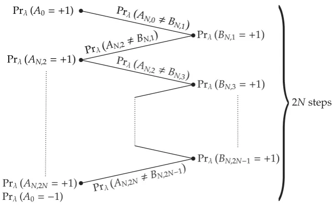
Before turning to the formal proof, the following should provide an intuition of the idea behind it. The correlation measure above is inspired by the use of
chained Bell inequalities, which were introduced in Pearle (1970) and Braunstein & Caves (1989). An important ingredient of chained Bell inequalities is that correlations are considered between outcomes when jointly measuring ˆOA
θ and
ˆ
OB
θ0, with a small difference betweenθandθ0. The correlation when jointly mea-suring two consecutive observables from the list ˆA0,BˆN,1, . . . ,BˆN,2N−1,AˆN,2N
gets stronger asNgets larger: Pr(AN,a6=BN,b) gets closer to 0, while the
differ-ence betweenθandθ0becomes smaller. Combining all the correlations between outcomes of consecutive observables, which is what happens in the definition of
IN in (4.19), an upper bound can be derived for the difference inλ-probabilities
of the outcomes for the first and the last observables, i.e. ˆA0and ˆAN,2N =−Aˆ0.
It turns out that as N gets larger, the correlations become so much stronger that theλ-probabilities for the values ofA0 and−A0 must be equal, i.e. they
must both equal 1/2. This is related to the fact that asN → ∞, each term in
IN is roughly proportional to 1/N2, while the number of terms is proportional
to N. Therefore,IN is roughly proportional to 1/N and goes to 0 in the limit.
This is illustrated in Figure 1.
Proceeding with the formal proof, omitting the superscript|φiAB for
nota-12In all summations involvingaandb, it is assumed thata∈ A
4 TRIVIALITY FOR BELL STATES 11
Prλ(A0= +1)
Prλ AN,2 = +1
Prλ A
N,0 BN ,1
Prλ AN,2
BN,1
Figure 1: The probabilities displayed at two subsequent points differ no more than the probability displayed at the line between these two points. Therefore, the difference between Prλ(A0 = +1) and Prλ(A0 = −1) is bounded above
by IN, which is the sum of 2N probabilities of the form Prλ(AN,a 6= BN,b)
with |a−b| = 1. The λ-average of each of these probabilities is smaller than
π2/(16N2). Therefore, the λ-averaged difference between Pr
λ(A0 = +1) and
Prλ(A0=−1) is bounded above by 2N π2/(16N2) =π2/(8N). Since this holds
for all N ∈ N, the λ-averaged difference equals zero, and therefore Prλ(A0 =
4 TRIVIALITY FOR BELL STATES 12
tional simplicity,
|Prλ(A0= 1)−Prλ(A0=−1)|=|Prλ(AN,0= 1)−Prλ(AN,2N = 1)|
≤ X
|a−b|=1
|Prλ(AN,a= 1)−Prλ(BN,b= 1)|
≤ X
|a−b|=1
Prλ(AN,a6=BN,b). (4.20)
The first inequality is a simple triangle inequality, while the second follows from an inequality in probability theory:
∀z∈Range(X)∩Range(Y) :
|Pr(X =z)−Pr(Y =z)|=|Pr(X =z, Y =z) + Pr(X =z, Y 6=z)
−Pr(X =z, Y =z)−Pr(X6=z, Y =z)| ≤Pr(X =z, Y 6=z) + Pr(X 6=z, Y =z)
≤Pr(X 6=Y). (4.21)
Note that we have assumed ParInd here: this gaurantees that, for example, Prλ(AN,a = 1) is well-defined and independent of what measurement is being
performed onB.
Integrating both sides of (4.20) using the measure µ(λ) gives, using Com-pQuant,
Z
Λ
dµ(λ)|Prλ(A0= 1)−Prλ(A0=−1)| ≤ Z
Λ
dµ(λ) X
|a−b|=1
Prλ(AN,a6=BN,b)
= X
|a−b|=1
Pr(AN,a6=BN,b) =IN.
(4.22)
IN is a sum of quantum-mechanical probabilities and can therefore be
calcu-lated:
a∈ AN, b∈ BN,|a−b|= 1⇒Pr|φiAB(AN,a=±1, BN,b=∓1) = 1/2 sin2
π
4N
,
so IN = 2Nsin2
π
4N
≤ π
2
8N ⇒ Nlim→∞IN = 0. (4.23)
Since (4.22) has to hold for all N, and the left-hand side is non-negative, it follows that
Z
Λ
dµ(λ)|Prλ(A0= 1)−Prλ(A0=−1)|= 0 ⇒ Prλ(A0= 1)
.
= Prλ(A0=−1).
(4.24)
Since both probabilities add up to 1, they both equal 1/2 almost everywhere. This can be written as13
Prλ [0]A
.
= Pr [0]A= 1/2; Prλ [1]A
.
= Pr [1]A
= 1/2. (4.25)
13The observable need not be specified here because in a 2-dimensional Hilbert space a
5 GENERALIZING TO HIGHER DIMENSIONAL STATE SPACES 13
In fact, for any other basis {|00iA,|10iA} of HA, there is a basis{|00iB,|10iB}
of HB such that|φiAB = √12(|00iA|00iB+|10iA|10iB).14 Therefore, (4.25) also
holds for measurements on Ain any other basis. We have proved triviality for the state |φiAB (4.16), in the 4-dimensional Hilbert spaceC2⊗C2.
5
Generalizing to higher dimensional state spaces
The result of the previous section can easily be generalized to maximally entan-gled states in higher dimensional state spaces. Consider a bipartite systemAB
in the state
|φdiAB:= d−1 X
i=0
ci|iiA|iiB ∈ HA⊗ HB=Cd⊗Cd, (5.26)
with ci ∈R+ for alli, d >2, and {|iiA}id=0−1 and{|iiB}di=0−1 orthonormal bases.
Consider a measurement onAin the basis{|iiA}di=0−1. We shall prove that equal
coefficients imply equalλ-probabilities:
∀j, k∈Nd: cj=ck ⇒ Prλ [j]A .
= Prλ [k]A. (5.27)
In particular, if all coefficients in (5.26) equal 1√d, all outcome probabilities equal 1/dalmost everywhere:
∀i∈Nd: Prλ [i]A
.
= 1
d = Pr [i]
A
. (5.28)
The proof is essentially the same as in the previous section: we focus on the two terms with equal coefficients and apply the same steps. Letcj and ck
be two equal coefficients. Similarly to the definitions (4.17) and (4.18) in the previous section, we define
|θi:= cos(θ/2)|ji+ sin(θ/2)|ki, θ∈[0, π]; ˆ
Oθ:=−1·[θ] + 1·[θ+π] +
X
i∈Nr\{j,k}
(i+ 2)·[i];
ˆ
AN,a:= ˆOAaπ/2N, a∈ AN;
ˆ
BN,b:= ˆOBbπ/2N, b∈ BN;
ˆ
A0:= ˆAN,0;
IN0 := X
|a−b|=1
Pr|φdiAB(A
N,a6=BN,b). (5.29)
Note that the observables ˆAN,0 and ˆAN,2N correspond to the measurement in
the basis{|iiA}di=0−1. Also, these observables are equal up to the exchange of the
eigenvalues +1 and −1, which means that AN,0 = ±1 iff AN,2N = ∓1. The
value ofIN0 is similar to that ofIN (4.19) in the previous section. The difference
14Namely, the basis{|00i
B,|10iB}, where |i0iB := Uij∗|jiB and Uij is the unitary matrix
5 GENERALIZING TO HIGHER DIMENSIONAL STATE SPACES 14
comes from the fact that the coefficients of the terms involving |jiA and |kiA
equal cj instead of 1
√
2:
IN0 = 4N c2jsin2 π 4N
≤ π
2c2
j
4N . (5.30)
Sincecj is constant,IN0 , likeIN, has the property limN→∞IN0 = 0. Repeating
the steps (4.20)–(4.24) gives
Prλ(A0= 1)
.
= Prλ(A0=−1). (5.31)
Using projectors, this can be expressed as
Prλ [j]A
A0 .
= Prλ [k]A
A0. (5.32)
Now, using the perfect correlation property (D.147) proven in Appendix D, settingI={j},
Prλ [j]A .
= Prλ [j]B, (5.33)
we get
Prλ [j]A
.
= Prλ [j]B
.
= Prλ [k]B
.
= Prλ [k]A
. (5.34)
Note that the perfect correlation also implies that these probabilities are inde-pendent of the observables. We now focus on the case with all coefficients equal to 1√d. Then, for any basis {|i0i
A}di=0−1 there is a basis {|i0iB}di=0−1 such that
|φdiAB =P d−1
i=0
1√
d|i0i
A|i0iB.15 It follows that for measurements in any
basis{|i0i
A}di=0−1 or{|i
0i
B}di=0−1:
∀i∈Nd: Prλ [i0]A .
=1
d = Pr [i
0]A
,
Prλ [i0]B .
=1
d = Pr [i
0]B
. (5.35)
In this case triviality also holds for measurements involving multidimensional projectors (or, equivalently, observables with degenerate eigenvalues). Consider a measurement on A involving the projector P
i∈J[i]
A, where J ⊂
Nd, and a
simultaneous measurement onB in the basis{|iiB}di=0−1. Then,
Prλ
X
i∈J
[i]A
!
.
=X
i∈J
Prλ [i]B .
=X
i∈J
1
d=
#J d = Pr
X
i∈J
[i]A
!
. (5.36)
Here we have made use of the perfect correlation property
Pr|φdiAB
λ
X
i∈J
[i]A
!
.
=X
i∈J
Pr|φdiAB
λ [i] B
, (5.37)
also proven in Appendix D. Remember that by ParInd, the outcome prob-abilities of a measurement performed on A are independent of whether any
15Namely, the basis{|i0i
B}di=0−1, where|i
0i
B:=Uij∗|jiB andUijis the unitary matrix such
6 GENERALIZING TO COEFFICIENTSC2
I ∈Q 15
measurement is performed on B. Therefore, while we did consider a specific measurement onB in (5.36), the result
Prλ
X
i∈J
[i]A
!
.
= Pr X
i∈J
[i]A
!
(5.38)
holds in general.
6
Generalizing to coefficients
c
2i∈
Q
In this section the result of the previous sections is generalized to states of which the Schmidt coefficients equal square roots of rational numbers:16
|φdiAB:= d−1 X
i=0
ci|iiA|iiB ∈ HA⊗ HB, (6.39)
where c2
i ∈ Q and ci > 0 for all i, d > 2, HA and HB are both at least of
dimension d, and {|iiA}id=0−1 and {|iiB}di=0−1 are sets of orthonormal vectors. 17
We shall prove that also in this case the λ-probabilities equal the quantum probabilities:
∀i∈Nd: Pr| φdiAB
λ [i] A .
= Pr|φdiAB [i]A
. (6.40)
The proof in this section is based on the following idea. System AB can be coupled to another system A0B0 such that the combined system AA0BB0
is approximately in a maximally entangled state. More precisely, for each i
the term|iiA|iiB is coupled to an approximate entangled state with a number
of terms that is proportional to c2i. To find these numbers, we consider the common denominator r of all fractions {c2
i} d−1
i=0, such that we can write c 2
i =
mi/r withmi∈N. The numeratorsmi are then proportional to c2i. Then, for
measurements on AA0BB0, which is approximately in a maximally entangled state, the result of the previous section can be applied. It turns out that this also puts constraints on the λ-probabilities for measurements on system AB
alone.
To produce the maximally entangled state, we assume the presence of yet another bipartite systemA00B00 that is prepared in a special ‘embezzling state’. The family of embezzling states was first introduced in van Dam & Hayden (2003), and they have the special property that any bipartite state can be ap-proximately extracted from it using local unitary operations (i.e. by applying separate unitary transformations onA00andB00). The precision of this operation can be enhanced by using an embezzling state of higher dimension.
Because we have to use the notion of ‘approximate states’ in this section, we define a distance measure for quantum states, called the trace distance:
D(|ψi,|φi) := (1/2)Tr
[ψ]−[φ]
, where (6.41)
|A|:=
√ A†A.
16The set of rational numbers is denoted by
Q.
17Since we allow for state spaces of dimension larger thand,{|ii
A}di=0−1 and{|iiB}di=0−1 do
6 GENERALIZING TO COEFFICIENTSC2
I ∈Q 16
As shown in Nielsen & Chuang (2004), the trace distance is a metric, and it provides an upper bound for the difference in quantum probabilities for the outcome associated with any projector ˆP:
hΨ|
ˆ
P|Ψi − hφ|P|φiˆ
≤D(|ψi,|φi). (6.42)
Also, for pure states the following relation holds between the trace distance and another distance measure, the fidelityF:
D(|ψi,|φi) =p1− F(|ψi,|φi)2,
whereF(|ψi,|φi) :=|hψ|φi|. (6.43)
Beginning with the proof, first define18
r:= LCD
c2i d−1
i=0
;
mi:=rc2i. (6.44)
The family of embezzling states{|τni}∞n=1 is defined as
|τni:=
1
√ Cn
n−1 X
j=0
1
√
j+ 1|ji ⊗ |ji ∈C
n⊗
Cn. (6.45)
Cn:=P n−1
j=0 1/(j+ 1) is a normalization constant, and{|ji}
n−1
j=0 an orthonormal
basis of Cn. System A00B00 is prepared in one of these states, indexed by n. Another systemA0B0 is prepared in a simple product state
|0iA0|0iB0 ∈ HA0⊗ HB0, (6.46)
where HA0 and HB0 are at least of dimension maxi∈
Ndmi. Taking all systems
together, the state before the measurement is
|Ψni:=|τniA00B00⊗ |0iA0|0iB0⊗ |φdiAB. (6.47)
Now, for each i, a maximally entangled state with Schmidt number mi is
extracted from the embezzling state, and coupled to the term |iiA|iiB. In
Appendix C it is shown that there are unitary operatorsUnAA0A00, UBB
0B00
n which
perform this task with a precision that increases asn→ ∞:
lim
n→∞D
UnAA0A00⊗UnBB0B00|Ψni,|χni
= 0, where (6.48)
|χni:=|τniA00B00⊗
d−1 X
i=0
r
mi
r |iiA|iiB
mi−1
X
j=0
1
√ mi
|jiA0|jiB0
=|τniA00B00⊗
d−1 X
i=0
mi−1
X
j=0
1
√
r|iiA|iiB|jiA0|jiB0
.
Here, {|jiA0}m−1
j=0 and {|jiB0}m−1
j=0 are sets of orthonormal vectors. Now
con-sider a measurement that consists of first performing the above unitary trans-formation, resulting approximately in a maximally entangled state for the sys-tem AA0BB0, and then measuring this system in the basis {|i, jiAA0}, where
6 GENERALIZING TO COEFFICIENTSC2
I ∈Q 17
|i, ji := |ii|ji. Note that, if the state UAA0A00
n ⊗UBB
0B00
n |Ψni is close to a
maximally entangled state, by (6.42) the outcome probabilities are also close to those of a maximally entangled state. Therefore, the result of the previous section can be applied. Actually, the unitary transformation can be included in the definition of the measurement projectors, because a unitary transformation applied to a complete set of orthogonal projectors gives another complete set of orthogonal projectors.
Define an index set containing all values of the pair (i, j) occurring in |χni:
Iind:=n(0,0),(0,1), . . . ,(0, m0−1),
(1,0), . . . ,(1, m1−1),
. . . ,
(d−1,0), . . . ,(d−1, md−1−1) o
. (6.49)
For (i1, j1),(i2, j2)∈Iinddefine, similarly to (5.29) in the previous section,19
|θi:= cos(θ/2)|i1, j1i+ sin(θ/2)|i2, j2i;
ˆ
Oθ:=−1·[θ] + 1·[θ+π] +
X
(i,j)∈Iind\{(i
1,j1),(i2,j2)}
2i3j+ 2
·[i, j];
ˆ
AN,n,a:=
UnAA0A00
−1
IA
00
⊗Oˆaπ/AA02N UnAA0A00, a∈ AN;
ˆ
BN,n,b:=
UnBB0B00
−1
IB
00
⊗Oˆbπ/BB20N UnBB0B00, b∈ BN;
ˆ
An,0:= ˆAN,n,0. (6.50)
Note that, as in the previous section, An,0 = ±1 iff AN,n,2N = ∓1. The use
of the expression (2i3j + 2) in the definition of ˆO
θ guarantees that distinct
eigenvalues are assigned to every projector [i, j], as in the previous section. Note that the observables ˆAand ˆB include the unitary operatorsUAA0A00
n and
UBB0B00
n , and therefore depend onn, which corresponds to the precision of the
embezzlement transformation.
Finally, a correlation measure is again defined, which now also depends on the precisionn:
IN,n:=
X
|a−b|=1
Pr|Ψni(A
N,n,a6=BN,n,b). (6.51)
This quantity has the property, similar to IN in the previous section, that it
vanishes when taking the limitsn→ ∞and then N→ ∞:
∀(i1, j1),(i2, j2)∈Iind: lim
N→∞nlim→∞IN,n= 0. (6.52)
The proof of (6.52) can be found in Appendix A.1. The correctness is already suggested by the fact thatIN,n consists of 2N probabilities, and as mentioned
above, those probabilities get closer to probabilities for a maximally entangled state asnincreases.
19While the symbols defined in (6.50) and (6.51) depend on the pairs (i
1, j1) and (i2, j2),
6 GENERALIZING TO COEFFICIENTSC2
I ∈Q 18
Analogously to the previous two sections, we have
Pr
|Ψni
λ (An,0= 1)−Pr
|Ψni
λ (An,0=−1)
= Pr
|Ψni
λ (AN,n,0= 1)−Pr
|Ψni
λ (AN,n,2N = 1)
≤ X
|a−b|=1 Pr
|Ψni
λ (AN,n,a= 1)−Pr
|Ψni
λ (BN,n,b= 1)
≤ X
|a−b|=1
Pr|Ψni
λ (AN,n,a6=BN,n,b).
(6.53)
Integrating with the measureµ(λ) gives
Z
Λ
dµ(λ) Pr
|Ψni
λ (An,0= 1)−Pr
|Ψni
λ (An,0=−1)
≤IN,n. (6.54)
Let >0. By (6.52), we can choosen, N such that for all (i1, j1),(i2, j2)∈Iind,
IN,n< , so that
∀(i1, j1),(i2, j2)∈Iind: Z
Λ
dµ(λ)
Pr
|Ψni
λ (An,0= 1)−Pr
|Ψni
λ (An,0=−1) < .
(6.55)
Defining the projector
ˆ
E(i,j),n:=
UnAA0A00
−1
IA
00
⊗[i, j]AA0 UnAA0A00, (6.56)
and noting that
ˆ
An,0=−1·Eˆ(i1,j1),n+ 1·Eˆ(i2,j2),n+. . . , (6.57)
we get, switching to the notation with projectors,
∀(i1, j1),(i2, j2)∈Iind: Z
Λ
dµ(λ)
Pr|Ψni
λ
ˆ
E(i2,j2),n
ˆ
An,0
−Pr|Ψni
λ
ˆ
E(i1,j1),n
ˆ
An,0
< . (6.58)
By CompQuant, we have
X
(i0,j0)∈Iind
Z
Λ
dµ(λ)Pr|Ψni
λ
ˆ
E(i0,j0),n
= 1 ⇒ X
(i0,j0)∈Iind
Pr|Ψni
λ
ˆ
E(i0,j0),n
.
= 1.
(6.59)
Using this, and a triangle inequality, we get
∀(i, j)∈Iind:
Z
Λ
dµ(λ)
Pr|Ψni
λ
ˆ
E(i,j),n
ˆ
An,0 −1 r = 1 r Z Λ
dµ(λ)
r·Pr|Ψni
λ
ˆ
E(i,j),n
ˆ
An,0
− X
(i0,j0)∈Iind
Pr|Ψni
λ
ˆ
E(i0,j0),n
ˆ
An,0
≤ 1 r X
(i0,j0)∈Iind
Z
Λ
dµ(λ)
Pr|Ψni
λ
ˆ
E(i,j),n
ˆ
An,0
−Pr|Ψni
λ
ˆ
E(i0,j0),n
ˆ
An,0
< #I
ind
r =.
7 GENERALIZING TO ARBITRARY COEFFICIENTS 19
Using a triangle inequality once more,
∀i∈Nd:
Z
Λ
dµ(λ)
mi−1
X
j=0
Pr|Ψni
λ
ˆ
E(i,j),n
ˆ
An,0 −mi
r ≤
mi−1
X
j=0 Z
Λ
dµ(λ)
Pr|Ψni
λ
ˆ
E(i,j),n
ˆ
An,0 −1 r
< mi. (6.61)
Using the correlation property
mi−1
X
j=0
Pr|Ψni
λ
ˆ
E(i,j),n
.
= Pr|Ψni
λ [i] B
, (6.62)
proven in Appendix D, we arrive at
∀i∈Nd:
Z
Λ
dµ(λ)
mi−1
X
j=0
Pr|Ψni
λ
ˆ
E(i,j),n
ˆ
An,0 −mi
r = Z Λ
dµ(λ) Pr
|Ψni
λ [i] B
−mi r
< mi. (6.63)
Since (6.63) holds for any > 0, we get, also applying (3.14) by noting that
|Ψni=|φdiAB⊗. . .,
Z
Λ
dµ(λ) Pr
|φdiAB
λ [i] B
−mi r
= 0
⇒ Pr|φdiAB
λ [i] B .
= mi
r =c
2
i = Pr|
φdiAB [i]B, (6.64)
which is the desired result.
Note that because of ParInd, once we have derived results for the proba-bilities for measurements on systemB using the correlation property and cer-tain measurements performed on system AA0A00, these results still hold when other measurements, or no measurements at all, are being performed on system
AA0A00.
Also note that, starting with the systemAA0A00BB0B00, withA00B00prepared
in an embezzling state, we have reached a conclusion about measurements on
AB, prepared in the pure state (6.39). Above we have applied (3.14), which states that the probabilities Pr|φdiAB
λ [i] B
are independent of the states of the systems A00B00 and A0B0. Therefore, while these systems were used for the derivation of (6.64), it follows that the result also holds without considering the systems A00B00andA0B0 in specially prepared states.
Like in the previous section, the result also holds withAandBinterchanged, and also for degenerate measurements.
7
Generalizing to arbitrary coefficients
Now suppose we have a state of the form
|φdiAB:= d−1 X
i=0
7 GENERALIZING TO ARBITRARY COEFFICIENTS 20
where ci ∈ R+ for all i, d > 2, HA and HB are both at least of dimension
d, and{|iiA}di=0−1and {|iiB}di=0−1 are sets of orthonormal vectors. Note that any
state can be written in this form by Schmidt’s decomposition theorem. Since we cannot generally write c2
i =mi/r withmi, r ∈N, the strategy of the previous section can not be applied. However, because the set of rational numbers is dense in the set of real numbers, the numbers c2
i can be approximated with
rational numbersc2
i,lby defining the sequences
(ci,l)∞l=1, with ∀i, l∈N:c 2
i,l∈Q, (7.66)
∀i: lim
l→∞ci,l=ci, (7.67)
∀l:
d−1 X
i=0
c2i,l= 1. (7.68)
As in the previous section, the idea is to apply a unitary transformation that results approximately in a maximally entangled state. But since the c2
i are
not rational numbers, we have to use the rational numbers c2
i,l to determine
the numerators and denominators for the unitary transformations. This time, to achieve any desired precision, not only nmust be chosen large enough, but also l. Again, the unitary transformation will be included in the measurement operators.
Instead of focussing on two terms, like we did in the previous section, the terms of the approximately maximally entangled state are now partitioned into two sets of equal size. Then, a measurement is considered using a projector that projects on the space spanned by one such set of terms, and measurements where this projector is ‘rotated’ by an angleθ. For a maximally entangled state, the quantum-mechanical statistics for such measurements are equal to those of the measurements on Bell states, considered in Section 4. Since we have a state that is close to a maximally entangled state, by (6.42) the quantum probabilities are also close to those of Bell states, i.e. close to 1/2. Using a similar derivation as in the previous two sections, it can be shown that also theλ-probabilities are close to 1/2. Then, using a lemma proved in Appendix B, we can also derive
λ-probabilities for projectors [i]A. In fact, those probabilities are again equal to
the quantum-mechanical ones for almost everyλ∈Λ.
For each l ∈ N, define rl as the least even common denominator of the
fractions{c2
i,l} d−1
i=0,20and let{mi,l}di=0−1 be the corresponding numerators:
rl:= LCD
c2i,l di=0−1∪ {1/2};
mi,l:=rlc2i,l. (7.69)
The reason thatrlneeds to be even is that an approximately maximally
entan-gled state with an even number of terms is needed in order to be able to divide the terms into two groups of equal size.
As in the previous section, we assume the presence of two extra bipartite systems, of which one is prepared in an embezzling state (6.45):
|Ψni:=|τniA00B00⊗ |0iA0|0iB0⊗ |φdiAB. (7.70)
7 GENERALIZING TO ARBITRARY COEFFICIENTS 21
Note that, for givenl,HA0 andHB0 are both at least of dimension maxi∈ Ndmi,l.
Again, define an index set:
Jlind:=n(0,0),(0,1), . . . ,(0, m0,l−1),
(1,0), . . . ,(1, m1,l−1),
. . . ,
(d−1,0), . . . ,(d−1, md−1,l−1)
o
. (7.71)
Note that Pd−1
i=0 mi,l = P d−1
i=0 rlc2i,l = rl by (7.69) and (7.68), and therefore
#Jind
l =rl.
LetJl⊂Jlindwith #Jl=rl/2; andpl:Jl→Jlind\Jlan arbitrary bijection.
Then, define
ˆ
OJAA0
l,θ := +1·
X
(i,j)∈Jl
[cos(θ/2)|i, jiAA0 + sin(θ/2)|pl(i, j)iAA0]
−1·
I
AA0
− X
(i,j)∈Jl
[cos(θ/2)|i, jiAA0+ sin(θ/2)|pl(i, j)iAA0]
;
ˆ
AJl,N,n,l,a:=
Un,lAA0A00
−1
IA
00
⊗OˆJAA;
l,aπ/2N U
AA0A00 n,l
, a∈ AN\{2N},
(7.72)
and ˆOBBJ 0
l,θ,
ˆ
BJl,N,n,l,banalogously. Furthermore, define
ˆ
AJl,n,l,0:= ˆAJl,N,n,l,0;
ˆ
AJl,N,n,l,2N :=−AˆJl,n,l,0. (7.73)
Now the correlation measure can be defined:
IJl,N,n,l:=
X
|a−b|=1
Pr|Ψni(A
Jl,N,n,l,a6=BJl,N,n,l,b). (7.74)
As shown in Appendix A.2, this measure has the property
lim
N→∞llim→∞nlim→∞IJl,N,n,l= 0. (7.75)
Now,
2
Pr
|Ψni
λ (AJl,n,l,0= +1)−1/2
=
Pr
|Ψni
λ (AJl,n,l,0= +1)−Pr
|Ψni
λ (AJl,n,l,0=−1)
= Pr
|Ψni
λ (AJl,N,n,l,0= +1)−Pr
|Ψni
λ (AJl,N,n,l,2N = +1)
≤ X
|a−b|=1 Pr
|Ψni
λ (AJl,N,n,l,a= +1)−Pr
|Ψni
λ (BJl,N,n,l,b= +1)
≤ X
|a−b|=1
Pr|Ψni
λ (AJl,N,n,l,a6=BJl,N,n,l,b)
7 GENERALIZING TO ARBITRARY COEFFICIENTS 22
Integrating with the measureµ(λ) gives
Z
Λ
dµ(λ)
Pr
|Ψni
λ (AJl,n,l,0= +1)−1/2
≤(1/2)IJl,N,n,l. (7.77)
Let > 0. By (7.75) and (7.67) we can choose N, l, n ∈ N such that for all
Jl⊂Jlindwith #Jl=rl/2,
Z
Λ
dµ(λ) Pr
|Ψni
λ (AJl,n,l,0= +1)−1/2
< ;
∀i∈Nd:|c2i,l−c2i|< . (7.78)
Now, define the projectors
ˆ
E(i,j),n,l:=
Un,lAA0A00
−1
[i, j]AA0⊗IA00 UAA0A00 n,l
,
ˆ
F(i,j),n,l:=
Un,lBB0B00
−1
[i, j]BB0⊗IB00 UBB0B00 n,l
. (7.79)
Noting that
ˆ
AJl,n,l,0= +1·
X
(i,j)∈Jl
ˆ
E(i,j),n,l
−1·
IAA 0A00
− X
(i,j)∈Jl
ˆ
E(i,j),n,l
, (7.80)
we switch to the notation with projectors, and using the correlation property (D.148),
Pr|Ψni
λ
X
(i,j)∈Jl
ˆ
E(i,j),n,l
.
= X
(i,j)∈Jl
Pr|Ψni
λ
ˆ
F(i,j),n,l
, (7.81)
we arrive at, for all Jl⊂Jlind with #Jl=rl/2,
Z
Λ
dµ(λ)
Pr|Ψni
λ
X
(i,j)∈Jl
ˆ
E(i,j),n,l
−1/2 < ⇒ Z Λ
dµ(λ)
X
(i,j)∈Jl
Pr|Ψni
λ
ˆ
F(i,j),n,l
−1/2
< . (7.82)
Now, we need the following lemma, proven in Appendix B:
Lemma 1. Let Λ be a measurable space with measure µ, let r be an even, positive integer, and let
n
pλiri=0−1
λ∈Λ
o
(7.83)
be some collection of sequences satisfying, for allI⊂Iind:=Nrwith#I=r/2,
Z
Λ
dµ(λ)
X
i∈I
pλi
!
−1/2
< . (7.84)
Then for allJ ⊂Iind
Z
Λ
dµ(λ)
X
i∈J
pλi
!
−#J /r
8 GENERALIZING TO ANY MEASUREMENT 23
Applying this lemma to the right-hand side of (7.82) with
pλiri=0−1≡Pr|Ψni
λ
ˆ
F(0,0),n,l
,Pr|Ψni
λ
ˆ
F(0,1),n,l
, . . . ,Pr|Ψni
λ
ˆ
F(d−1,md−1,l),n,l
,
(7.86)
we get, for alli∈Nd,
Z
Λ
dµ(λ)
mi,l−1
X
j=0
Pr|Ψni
λ
ˆ
F(i,j),n,l
−mi,l rl
<2. (7.87)
Again, applying perfect correlation (D.150),
mi,l−1
X
j=0
Pr|Ψni
λ
ˆ
F(i,j),n,l
.
= Pr|Ψni
λ [i] A
, (7.88)
and noting thatmi,l/rl=c2i,lby (7.69), we obtain, also using (3.14),
Z
Λ
dµ(λ) Pr
|φdiAB
λ [i] A
−c2i,l
<2. (7.89)
Finally, using the triangle inequality|x−y| ≤ |x−z|+|z−y|
Z
Λ
dµ(λ) Pr
|φdiAB
λ [i] A
−c2i
≤
Z
Λ
dµ(λ) Pr
|φdiAB
λ [i] A
−c2i,l +
Z
Λ
dµ(λ)c2i,l−c2i
<3, (7.90)
and since the inequality holds for all >0, we get
Z
Λ
dµ(λ) Pr
|φdiAB
λ [i] A
−c2i = 0
⇒Pr|φdiAB
λ [i] A .
=c2i = Pr|
φdiAB [i]A, (7.91)
which is the desired result. Again, the result also holds with A and B inter-changed, and also for degenerate measurements.
8
Generalizing to any measurement
In the above sections, we considered measurements on subsystems of bipartite systems in entangled states. However, since in fact every measurement involves such entanglement, something can also be said about general measurements. In this section, we show how this can be done.21 This generalization is performed
step-by-step, by considering three types of measurements in turn: measurements of the first kind, measurements of the second kind, and POVM22measurements.
21The results of this section are largely based on a suggestion made by Guido Bacciagaluppi
(private communication).
22POVM stands for Positive Operator-Valued Measure. A detailed treatment of these
8 GENERALIZING TO ANY MEASUREMENT 24
8.1
Measurements of the first kind
The measurement process can be divided into two steps. First, the system to be measured is coupled to the measurement apparatus, which results in entangle-ment between the system and the apparatus. Then, the measureentangle-ment result is read off the measurement apparatus. In the case of a measurement of the first kind with projectors{EˆjA}dj=0−1, the coupling has the following form:
|ψiA|0iB = d−1 X
j=0
ˆ
EAj|ψiA|0iB7→ d−1 X
j=0
ˆ
EjA|ψiA|jiB= d−1 X
j=0
cj|jiA|jiB, (8.92)
where
|jiA:=
ˆ
EA j |ψiA
ˆ
EjA|ψiA
, and cj :=|hj|ψiA|=
ˆ
EjA|ψiA
, (8.93)
|iiB are (mutually orthogonal) ‘pointer states’, and|0iB is the so-called ‘ready
state’ of the measurement apparatus before measuring. The reading out of the measurement apparatus can then be described as a measurement performed on the apparatus in the ‘pointer basis’:
PrPdj−=01cj|jiA|jiB [i]B. (8.94)
Note that these probabilities equal the probabilities of the original measure-ment on systemA, as they should, because both measurements are actually two different descriptions of a single measurement:
Pr|ψiAEˆA
i
= PrPdj−=01cj|jiA|jiB [i]B
. (8.95)
Since these probabilities are equal by definition, the same relation holds when consideringλ-probabilities:
Pr|ψiA
λ
ˆ
EiA
ˆ
OA= Pr
Pd−1
j=0cj|jiA|jiB
λ [i]
B ˆ
OB, (8.96)
where ˆOBis an observable that includes the pointer states as eigenstates. Now, to the probability on the right-hand side of the above equation the result of Section 7 can be applied. Therefore, for any measurement of the first kind, the
λ-probabilities are trivial:23
Pr|ψiA
λ
ˆ
EiA= Pr. |ψiAEˆA
i
=c2i. (8.97)
23More generally, the measurement on the apparatus may involve one or more
multidi-mensional projectors onHB that each have multiple pointer states as eigenstates. If this is
the case, this corresponds to a degenerate measurement on system Awhere, for each such projector onHB, the projectors{EˆjA}corresponding to these pointer states are summed to
obtain the projector onHA corresponding to the projector onHB (like ˆEAi corresponds to
[i]Bin (8.95) and (8.96)). The result of Section 7, also holding for degenerate measurements,
still applies. The same considerations apply to the measurements considered in the next two subsections, where in Section 8.3 not projectors, but positive operators{FˆA
8 GENERALIZING TO ANY MEASUREMENT 25
8.2
Measurements of the second kind
In measurements of the second kind, the coupling between system and mea-surement apparatus is more general. When a meamea-surement of the first kind is performed, a system initially in an eigenstate of the observable remains in that same eigenstate after the measurement. In contrast, when a measurement of the second kind is performed, such a system may end up in a different state. Therefore, the coupling is as follows:
|ψiA|0iB= d−1 X
j=0
ˆ
EjA|ψiA|0iB 7→ d−1 X
j=0
cj|jiA|jiB (8.98)
where cj is as in (8.95), but now the states |jiA can be anything and are in
general not mutually orthogonal. This prevents the direct application of the result of Section 7 to the right-hand side of (8.98). However, the measurement apparatus can generally be decomposed into subsystems which get entangled with each other during the measurement (for example, different particles of a pointer). Or, the measurement apparatus may interact with another system be-fore any interaction with the experimenter takes place (for example, a computer recording the outcome). In this case, we can write HB ≡ HB1⊗ HB2, and we
have the coupling
|ψiA|0iB1|0iB2= d−1 X
j=0
ˆ
EjA|ψiA|0iB1|0iB2 7→ d−1 X
j=0
cj|jiA|jiB1|0iB2 7→ d−1 X
j=0
cj|jiA|jiB1|jiB2.
(8.99)
Here, the states|jiB1 are mutually orthogonal, as are the states|jiB2. Writing |jiAB1 ≡ |jiA|jiB1, theλ-probabilities of the measurement are now given by
Pr
Pd−1
j=0cj|jiAB1|jiB2
λ [i]
B2
ˆ
OB2 (8.100)
and, noting that the states |jiAB1 are mutually orthogonal, we see that again
the result of Section 7 can be applied to it, resulting again in (8.97).
8.3
POVM measurements
The result can also be extended to POVM measurements. In the case of such a measurement, the coupling is even more general. It is characterized by a complete set of positive operators{FˆA
j } d−1
j=0, which do not have to be projection
operators. In this case the coupling to the measurement apparatus is as follows:
|ψiA|0iB7→ d−1 X
j=0
ˆ
MjA|ψiA|jiB = d−1 X
j=0
cj|jiA|jiB, (8.101)
where
|jiA:=
ˆ
MA j |ψiA
ˆ
MA j |ψiA
, and cj:=|hj|ψiA|=
ˆ
MjA|ψiA
, (8.102)
and the ˆMA
9 DISCUSSION 26
As in the case of measurements of the second kind, the measurement ap-paratus can generally be decomposed into two subsystems which get entangled during the measurement process:
|ψiA|0iB1|0iB2= d−1 X
j=0
ˆ
MjA|ψiA|0iB1|0iB27→ d−1 X
j=0
cj|jiA|jiB1|0iB2 7→ d−1 X
j=0
ci|jiA|jiB1|jiB2.
(8.103)
Again, by writing|jiAB1 ≡ |jiA|jiB1 we end up withλ-probabilities
Pr
Pd−1
j=0cj|jiAB1|jiB2
λ [i]
B2
ˆ
OB2 (8.104)
to which the result of Section 7 can be applied, so that we get
Pr|ψiA
λ
ˆ
FiA= Pr. |ψiAFˆA
i
=c2i. (8.105)
9
Discussion
We summarize the main differences between the deduction presented in this article and C&R’s derivation:
• As mentioned in the Introduction, C&R define their ‘Freedom of Choice’ assumption in such a way that they can deduce ‘no-signalling’, which is similar to ParInd, from it (Section VII.A).24Instead, we explicitly assume
ParInd, whereby there entire issue of deducing ParInd from a freedom assumption becomes irrelevant.
• The proof in Section 4 is considerably simplified compared with that of C&R (Section VII.B).
• The result of Section 5 is not present in C&R’s work. Instead, C&R pre-sume that the result of Section 4 can be extended to maximally entangled states of Schmidt number 2n, by consideringncopies of a system in a Bell
state (Section VII.C). Note that results similar to that of Section 5 have been derived in Leifer (2014), Ghirardi & Romano (2012) and Barrett et al. (2006).
• Before generalizing to states with arbitrary Schmidt coefficients in Sec-tion 7, we consider states with Schmidt coefficients that are square roots of rational numbers in Section 6. C&R did not perform this intermediate step, and only considered transforming the state approximately to a max-imally entangled state with Schmidt number 2n. Then, they applied the
result for Bell states (Section 4), without justifying how this result can be applied to approximate states (Section VII.C). Actually, filling this gap is problematic, and therefore in this article a whole different approach, not present in C&R’s work, is introduced to prove the result, including defining the correlation measures for approximate statesIN,nandIJl,N,n,l
and proving Lemma 1 in Appendix B.
24Sections denoted using Roman numerals are sections in Colbeck & Renner (2012b).