Strawberry Fields: A Software Platform for Photonic Quantum Computing

Strawberry Fields:

A Software Platform for Photonic Quantum Computing

Nathan Killoran, Josh Izaac, Nicolás Quesada, Ville Bergholm, Matthew Amy, and

Christian Weedbrook

Xanadu, 372 Richmond St W, Toronto, M5V 1X6, Canada

We introduce Strawberry Fields, an open-source quantum programming architecture for light-based quantum computers,

and detail its key features. Built in Python, Strawberry Fields is a full-stack library for design, simulation, optimization, and

quantum machine learning of continuous-variable circuits. The platform consists of three main components: (i) an API for

quantum programming based on an easy-to-use language named Blackbird; (ii) a suite of three virtual quantum computer

backends, built in NumPy and TensorFlow, each targeting specialized uses; and (iii) an engine which can compile

Black-bird programs on various backends, including the three built-in simulators, and – in the near future – photonic quantum

information processors. The library also contains examples of several paradigmatic algorithms, including teleportation,

(Gaussian) boson sampling, instantaneous quantum polynomial, Hamiltonian simulation, and variational quantum circuit

optimization.

Introduction

The decades-long worldwide quest to build practical quantum computers is currently undergoing a critical pe-riod. During the next few years, a number of different quantum devices will become available to the public. While fault-tolerant quantum computers will one day provide sig-nificant computational speedups for problems like factor-ing[1], search[2], or linear algebra[3], near-term quan-tum devices will be noisy, approximate, and sub-universal [4]. Nevertheless, these emerging quantum processors are expected to be strong enough to show a computational ad-vantage over classical computers for certain problems, an achievement known as quantum computational supremacy. As we approach this milestone, work is already under-way exploring how such quantum processors might best be leveraged. Popular techniques include variational quan-tum eigensolvers [5, 6], quantum approximate optimiza-tion algorithms[7,8], sampling from computationally hard probability distributions [9–17], and quantum annealing [18,19]. Notably, these methodologies can be applied to tackle important practical problems in chemistry[20–23], finance_[24_], optimization_[25,26_], and machine learning [27–34]. These known applications are very promising, yet it is perhaps theunknownfuture applications of quantum computers that are most tantalizing. We may not know the best applications of quantum computers until these devices become available more widely to researchers, students, en-trepreneurs, and programmers worldwide.

To this end, a nascent quantum software ecosystem has recently begun to develop [35–47]. However, a

prevail-ing theme for these software efforts is to target qubit-based quantum devices. In reality, there are several com-peting models of quantum computing which are equiva-lent in computational terms, but which are conceptually quite distinct. One prominent approach is the continuous variable (CV) model of quantum computing [48–50]. In the CV model, the basic information-processing unit is an infinite-dimensional bosonic mode, making it particularly well-suited for implementations and applications based on light. The CV model retains the computational power of the qubit model (cf. Chap. 4 of Ref.[51]), while offering a number of unique features. For instance, the CV model is a natural fit for simulating bosonic systems (electromagnetic fields, trapped atoms, harmonic oscillators, Bose-Einstein condensates, phonons, or optomechanical resonators) and for settings where continuous quantum operators – such as position & momentum – are present. Even in classical com-puting, recent advances from deep learning have demon-strated the power and flexibility of a continuous represen-tation of compurepresen-tation[52,53]in comparison to the discrete computational model which has historically dominated.

Here we introduce Strawberry Fields1_{, an open-source}

software architecture for photonic quantum computing. Strawberry Fields is a full-stack quantum software plat-form, implemented in Python, specifically targeted to the CV model. Its main element is a new quantum program-ming language named Blackbird. To lay the groundwork for future photonic quantum computing hardware,

Straw-1_{This document refers to Strawberry Fields version 0.9. Full}

documenta-tion is available online atstrawberryfields.readthedocs.io.

berry Fields also includes a suite of three CV quantum simu-lator backends implemented using NumPy_[54_]and Tensor-Flow[55]. Strawberry Fields comes with a built-in engine to convert Blackbird programs to run on any of the simula-tor backends or, when they are available, on photonic quan-tum computers. To accompany the library, an online service for interactive exploration and simulation of CV circuits is available atstrawberryfields.ai.

Aside from being the first quantum software frame-work to support photonic quantum computation with continuous-variables, Strawberry Fields provides additional computational features not presently available in the quan-tum software ecosystem:

1. We provide two numeric simulators; a Gaussian back-end, and a Fock-basis backend. These two formula-tions are unique to the CV model of quantum compu-tation due to the use of an infinite Hilbert space, and came with their own technical challenges.

(a) The Gaussian backend provides state-of-the-art methods and functions for calculating the fi-delity and Fock state probabilities, involving cal-culations of the classically intractable hafnian [56].

(b) The Fock backend allows operations such as squeezing and beamsplitters to be performed in the Fock-basis, a computationally intensive calculation that has been highly vectorized and benchmarked for performance.

2. We provide a suite of important circuit decomposi-tions appearing in quantum photonics – such as the Williamson, Bloch-Messiah, and Clements decompo-sitions.

3. The Fock-basis backend written using the TensorFlow machine learning library allows for symbolic calcu-lations, automatic differentiation, and backpropaga-tion through CV quantum simulabackpropaga-tions. As far as we are aware, this is the first quantum simulation library written using a high-level machine learning library, with support for dataflow programming and auto-matic differentiation.

The remainder of this white paper is structured as fol-lows. Before presenting Strawberry Fields, we first provide a brief overview of the key ingredients for CV quantum com-putation, specifically the most important states, gates, and measurements. We then introduce the Strawberry Fields ar-chitecture in full, presenting the Blackbird quantum assem-bly language, outlining how to use the library for numerical simulation, optimization, and quantum machine learning. Finally, we discuss the three built-in simulators and the in-ternal representations that they employ. In the Appendices, we give further mathematical and software details and pro-vide full example code for a number of important CV quan-tum computing tasks.

Quantum Computation with Continuous

Variables

Many physical systems in nature are intrinsically contin-uous, with light being the prototypical example. Such sys-tems reside in an infinite-dimensional Hilbert space, offer-ing a paradigm for quantum computation which is distinct from the discrete qubit model. This continuous-variable model takes its name from the fact that the quantum op-erators underlying the model have continuous spectra. It is possible to embed qubit-based computations into the CV picture[57], so the CV model is as powerful as its qubit counterparts.

From Qubits to Qumodes

A high-level comparison of CV quantum computation with the qubit model is depicted in TableI. In the remainder of this section, we will provide a basic presentation of the key elements of the CV model. A more detailed technical overview can be found in AppendixA. Readers experienced with CV quantum computing can safely skip to the next sec-tion.

CV Qubit

Basic element Qumodes Qubits

Relevant operators

Quadratures ˆx, ˆp Mode operators ˆa, ˆa†

Pauli operators ˆ

σx, ˆσy, ˆσz

Common states

Coherent states|α〉

Squeezed states|z〉

Number states|n〉

Pauli eigenstates

|0/1〉,|±〉,|±i〉

Common gates

Rotation, Displacement, Squeezing, Beamsplitter, Cubic Phase

Phase shift, Hadamard, CNOT, T-Gate

Common measurements

Homodyne|x_φ〉〈x_φ|, Heterodyne1_π|α〉〈α|, Photon-counting|n〉〈n|

Pauli eigenstates

|0/1〉〈0/1|,|±〉〈±|,

| ±i〉〈±i|

Table I:Basic comparison of the CV and qubit settings.

The most elementary CV system is the bosonic harmonic oscillator, defined via the canonical mode operators ˆaand ˆ

oper-ators)2_,

ˆ x:=

v t_ħh

2(ˆa+aˆ

†_{), (1)}

ˆ p:=−i

v t_ħh

2(ˆa−aˆ

†_{), (2)}

where[ˆx, ˆp] =iħhˆI. We can picture a fixed harmonic oscil-lator mode (say, within an optical fibre or a waveguide on a photonic chip) as a single ‘wire’ in a quantum circuit. These qumodesare the fundamental information-carrying units of CV quantum computers. By combining multiple qumodes – each with corresponding operators ˆaiand ˆa†i – and

interact-ing them via sequences of suitable quantum gates, we can implement a general CV quantum computation.

CV States

The dichotomy between qubit and CV systems is perhaps most evident in the basis expansions of quantum states:

Qubit |φ〉=φ0|0〉+φ1|1〉, (3)

Qumode |ψ〉= Z

d x ψ(x)|x〉. (4)

For qubits, we use a discrete set of coefficients; for CV sys-tems, we can have acontinuum. The states|x_〉are the eigen-states of the ˆxquadrature, ˆx|x〉=x|x〉, withx∈R. These quadrature states are special cases of a more general family of CV states, theGaussian states, which we now introduce.

Gaussian states

Our starting point is the vacuum state|0〉. Other states can be created by evolving the vacuum state according to

|ψ〉=exp(−i t H)|0〉, (5)

whereH is a bosonic Hamiltonian (i.e., a function of the operators ˆai and ˆa†i) and t is the evolution time. States

where the HamiltonianH is at most quadratic in the oper-ators ˆaiand ˆa†i (equivalently, in ˆxiand ˆpi) are called

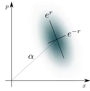
Gaus-sian. For a single qumode, Gaussian states are parameter-ized by two continuous complex variables: a displacement parameter α ∈ C and a squeezing parameter z ∈ C (of-ten expressed as z = rexp(iφ), with r ≥ 0). Gaussian states are so-named because we can identify each Gaussian state with a corresponding Gaussian distribution. For single qumodes, the identification proceeds through its displace-ment and squeezing parameters. The displacedisplace-ment gives

2_{It is common to picture} ħ

has a (dimensionless) scaling parameter for the ˆxand ˆpoperators rather than a physical constant. However, there are several conventions for the scaling value in common use [58]. These self-adjoint operators are proportional to the Hermitian and anti-Hermitian parts of the operator ˆa. Strawberry Fields allows the user to specify this value, with the defaultħh=2.

FIG. 1:Schematic representation of a Gaussian state for a single mode. The shape and orientation are parameterized by the displacementαand squeezing z=rexp(iφ).

the centre of the distribution, while the squeezing deter-mines the variance and rotation of the distribution (see Fig. 1). Multimode Gaussian states, on the other hand, are pa-rameterized by a vector of displacements ¯rand a covariance matrixV. Many important pure states in the CV model are special cases of the pure Gaussian states; see TableIIfor a summary.

State family Displacement Squeezing

Vacuum state|0〉 α=0 z=0

Coherent states|α〉 α∈C z=0

Squeezed states|z〉 α=0 z∈C

Displaced squeezed

states|α,z〉 α∈C z∈C

ˆ

xeigenstates|x〉 α∈C,

x₌2qħh

2Re(α)

φ=0,r→ ∞

ˆ

peigenstates|p〉 α∈C,

p=2qħh

2Im(α)

φ=π,r→ ∞

Fock states|n〉 N.A. N.A.

Table II:Common single-mode pure states and their relation to the displacement and squeezing parameters. All listed families are Gaussian, except for the Fock states. The n=0 Fock state is also the vacuum state.

Fock states

the form

|α〉=exp€−|α2|2 ŠX∞

n=0 αn

p

n!|n〉, (6)

while (undisplaced) squeezed states only have even number states in their expansion:

|z〉= p 1 coshr

∞ X

n=0 p

(2n)! 2n_n! [−e

iφ_tanh(r)]n

|2n〉. (7)

Mixed states

Mixed Gaussian states are also important in the CV pic-ture, for instance, thethermal state

ρ(n):=

∞ X

n=0 nn

(1+n)n+1|n〉〈n|, (8)

which is parameterized via the mean photon numbern:= Tr(ρ(n)nˆ). Starting from this state, we can consider a mixed-state-creation process similar to Eq. (5), namely

ρ=exp(−i t H)ρ(n)exp(i t H). (9)

Analogously to pure states, by applying Hamiltonians of second-order (or lower) to thermal states, we generate the family of Gaussian mixed states.

CV Gates

Unitary operations can be associated with a generating HamiltonianH via the recipe (cf. Eqs. (5) & (9))

U:=exp(−i t H). (10)

For convenience, we classify unitaries by the degree of their generator. A CV quantum computer is said to be universal if it can implement, to arbitrary precision and with a finite number of steps, any unitary which is polynomial in the mode operators[48]. We can build a multimode unitary by applying a sequence of gates from auniversal gate set, each of which acts only on one or two modes. We focus on a universal set made from the following two subsets:

Gaussian gates: Single and two-mode gates which are at most quadratic in the mode operators, e.g., Displace-ment, Rotation, Squeezing, and Beamsplittergates.

Non-Gaussian gate: A single-mode gate which is degree 3 or higher, e.g., theCubic phasegate.

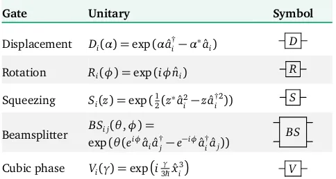
A number of fundamental CV gates are presented in Ta-bleIII. Many of the Gaussian states from the previous sec-tion are connected to a corresponding Gaussian gate. Any multimode Gaussian gate can be implemented through a suitable combination of Displacement, Rotation, Squeezing, and Beamsplitter Gates[50], making these gates sufficient for constructing all quadratic unitaries. The cubic phase gate is presented as an exemplary non-Gaussian gate, but any other non-Gaussian gate could also be used to achieve

universality. A number of other useful CV gates are listed in AppendixB.

Gate Unitary Symbol

Displacement Di(α) =exp(αaˆ

†

i −α∗ˆai) D

Rotation Ri(φ) =exp(iφnˆi) R

Squeezing Si(z) =exp(

1 2(z∗ˆa

2

i −zˆa

†2

i )) S

Beamsplitter BSi j(θ,φ) = exp(θ(eiφ_aˆ

iaˆ

†

j−e− iφ_aˆ†

iˆaj))

BS

Cubic phase Vi(γ) =exp i

γ 3ħhˆx

3

i

V

Table III:Some important CV model gates. All listed gates except the cubic phase gate are Gaussian.

CV Measurements

As with CV states and gates, we can distinguish between Gaussian and non-Gaussian measurements. The Gaus-sian class consists of two (continuous) types: homodyne and heterodyne measurements, while the key non-Gaussian measurement is photon counting. These are summarized in TableIV.

Homodyne measurements

Ideal homodyne detection is a projective measurement onto the eigenstates of the quadrature operator ˆx. These states form a continuum, so homodyne measurements are inherently continuous, returning valuesx ∈R. More gen-erally, we can consider projective measurement onto the eigenstatesx_φ

of the Hermitian operator

ˆ

x_φ:=cosφ ˆx+sinφ ˆp. (11)

This is equivalent to rotating the state clockwise byφand performing an ˆx-homodyne measurement. If we have a multimode Gaussian state and we perform homodyne mea-surement on one of the modes, the conditional state of the unmeasured modes remains Gaussian.

Heterodyne measurements

Measurement Measurement Operators

Measurement values

Homodyne |x_φ〉〈x_φ| x∈R

Heterodyne 1_π|α〉〈α| α∈C

Photon counting |n〉〈n| n∈N

Table IV:Key measurement types for the CV model. The ‘-dyne’ measurements are Gaussian, while photon-counting is non-Gaussian.

Photon Counting

Photon counting (also known as as photon-number re-solving measurement), is a complementary measurement method to the ‘-dyne’ measurements, revealing the particle-like, rather than the wave-particle-like, nature of qumodes. This measurement projects onto the number eigenstates|n〉, re-turning non-negative integer valuesn∈N. Except for the outcomen=0, a photon-counting measurement on a sin-gle mode of a multimode Gaussian state will cause the re-maining modes to become non-Gaussian. Thus, photon-counting can be used as an ingredient for implementing non-Gaussian gates. A related process is photodetection, where a detector only resolves the vacuum state from non-vacuum states. This process has only two measurement op-erators, namely|0〉〈0|andI− |0〉〈0|.

The Strawberry Fields Software Platform

The Strawberry Fields library has been designed with sev-eral key goals in mind. Foremost, it is a standard-bearer for the CV model, laying the groundwork for future photonic quantum computers. As well, Strawberry Fields is designed to be simple to use, giving entry points for as many users as possible. Finally, since the potential applications of near-term quantum computers are still being worked out, it is important that Strawberry Fields provides powerful tools to easily explore many different use-cases and applications. Strawberry Fields has been implemented in Python, a modern language with a gentle learning curve which is al-ready familiar to many programmers and scientific practi-tioners. The accompanying quantum simulator backends are built upon the widely used Python packages NumPy and TensorFlow. All Strawberry Fields code is open source. Strawberry Fields can be accessed programmatically as a Python package, or via a browser-based interface for de-signing quantum circuits.

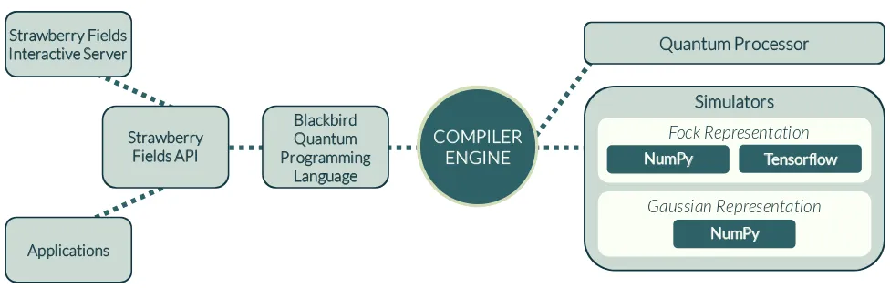
A pictorial outline of Strawberry Fields’ key elements and their interdependencies is presented in Fig. 2. Conceptu-ally, the software stack is separated into two main pieces: a user-facing frontend layer and a lower-level backends com-ponent. The frontend encompasses the Strawberry Fields Python API and the Blackbird quantum assembly language.

These elements provide access points for users to design quantum circuits. These circuits are then linked to a back-end via a quantum compiler engine. For a backback-end, the engine can currently target one of three included quantum computer simulators. When CV quantum processors be-come available in the near future, the engine will also build and run circuits on those devices. Further, high-level quan-tum computing applications can be built by leverging the Strawberry Fields frontend API. Existing examples include the Strawberry Fields Interactive website, the Quantum Ma-chine Learning Toolbox (for streamlining the training of variational quantum circuits), and SFOpenBoson (an inter-face between the electronic structure library OpenFermion [45]and Strawberry Fields).

In the remainder of this section, the key elements of Strawberry Fields will be presented in more detail. Proceed-ing through a series of examples, we show how CV quantum computations can be defined using the Blackbird language, then compiled and run on a quantum computer backend. We also outline how to use Strawberry Fields for optimiza-tion and machine learning on quantum circuits. Finally, we discuss the suite of quantum computer simulators included within Strawberry Fields.

Blackbird: A Quantum Programming Language

As classical computers have become progressively more powerful, the languages used to program them have also undergone considerable paradigmatic changes. Machine code gave way to human-readable assembly languages, fol-lowed by higher-level procedural and object-oriented lan-guages. With each generation, the trend has been towards higher levels of abstraction, separating the programmer more and more from details of the actual computer hard-ware. Quantum computers are still at an early stage of development, so while we can imagine what higher-level quantum programming might look like, in the near term we first need to build languages which are conceptually closer to the quantum hardware.

Blackbird is a standalone domain specific language (DSL) for continuous-variable quantum computation. With a well-defined grammar in extended Backus-Naur form, and both Python and C++parsers available, Blackbird provides op-erations that match the basic CV states, gates, and mea-surements, and maps directly to low-level hardware instruc-tions. The abstract syntax keeps a close connection between code and the quantum operations that they implement; this syntax is modeled after that of ProjectQ[41], but special-ized to the CV setting. Blackbird can be used as part of the Strawberry Fields stack, but also directly with photonic quantum computing hardware systems.

COMPILER ENGINE

BACK-ENDS

FRONT-ENDS

Strawberry Fields Interactive Server

Applications

Strawberry Fields API

Blackbird Quantum Programming

Language

Quantum Processor

Simulators

Fock Representation

Gaussian Representation

NumPy Tensorflow

NumPy

FIG. 2:Outline of the Strawberry Fields software stack. The Strawberry Fields Interactive server is available online at

strawberryfields.ai.

quantum operations that are decomposed into lower-level Blackbird assembly commands. We will introduce the ele-ments of Blackbird through a series of basic examples, dis-cussing more technical aspects as they arise.

Operations

Quantum computations consist of four main ingredients: state preparations, application of gates, performing mea-surements, and adding/removing subsystems. In Blackbird, these are all considered asOperations, and share the same basic syntax. In the following code examples, we use the variable

q

for a set of qumodes (more specifically, a quan-tum register), the details of which are deferred until the next section.

Our first considered Operation is state preparation. By default, qumodes are initialized in the vacuum state. Var-ious other important CV states can be created with simple Blackbird commands.

1 # Create the vacuum state in qumode 0 2 Vac | q[0]

3

4 # Create a coherent state in qumode 1 5 alpha = 2.0 + 1j

6 Coherent(alpha) | q[1]

7

8 # Create squeezed states in qumodes 0 & 1 9 S = Squeezed(2.0)

10 S | q[0] 11 S | q[1]

12

13 # Create a Fock state in qumode 1 14 Fock(4) | q[1]

Codeblock 1: Blackbird code for creating various CV quantum states.

Blackbird state preparations such as those used in Code-block 1 implicitly reset the existing state of the qumodes.

Conceptually, the vertical bar symbol ‘|’ separates Opera-tions – like state preparation – from the registers that they act upon. Notice that we can use Operations inline, or con-struct them separately and reuse them several times.

After creating states, we will want to transform these us-ing quantum gates.

1 # Apply the Displacement gate to qumode 0 2 alpha = 2.0 + 1j

3 Dgate(alpha) | q[0]

4

5 # Apply the Rotation gate 6 phi = 1.157

7 Rgate(phi) | q[0] 8

9 # Apply the Squeezing gate 10 Sgate(2.0, 0.17) | q[0] 11

12 # Apply the Beamsplitter gate to qumodes 0 & 1 13 BSgate(0.314, 0.223) | (q[0], q[1])

14

15 # Apply Cubic phase gate (VGate) to qumode 0 16 gamma = 0.1

17 Vgate(gamma) | q[0] 18

19 # Apply Hermitian conjugate of a gate 20 V = Vgate(gamma)

21 V.H | q[0]

Codeblock 2:Blackbird code for applying various CV gates. Blackbird supports all of the gates listed in the previous sec-tion as well as a number of composite gates, each of which can be decomposed using the universal gates. The sup-ported composite gates are: controlled X (CXgate), con-trolled Z (CZgate), quadratic phase (Pgate), and two-mode squeezing (S2gate). A full list of gates currently supported in Blackbird can be found in AppendixB.

1 # Homodyne measurement at angle phi 2 phi = 0.785

3 MeasureHomodyne(phi) | q[0]

4

5 # Special homodyne measurements 6 MeasureX | q[0]

7 MeasureP | q[1]

8

9 # Heterodyne measurement 10 MeasureHeterodyne() | q[0]

11 MeasureHD | q[1] # shorthand 12

13 # Number state measurements of various qumodes 14 MeasureFock() | q[0]

15 MeasureFock() | (q[1], q[2]) # multiple modes 16 Measure | q[3] # shorthand

Codeblock 3: Blackbird code for carrying out CV measurements.

Measurements have several effects. For one, the numeri-cal result of the measurement is placed in a classinumeri-cal regis-ter. As well, the state of all remaining qumodes is projected to the (normalized) conditional state for that measurement value. Finally, the state of the measured qumode is reset to the vacuum state. This is the typical behaviour of pho-tonic hardware, where measurements absorb all the energy of the measured qumode.

Running Blackbird Programs in Python

Within Python, Blackbird programs are managed by an Engine. The function

Engine

in the Strawberry Fields API will instantiate an Engine, returning both the Engine and its corresponding quantum register. The Engine is used as a Python context manager, providing a convenient way to encapsulate Blackbird programs.

1 # Create Engine and quantum register 2 import strawberryfields as sf

3 eng, q = sf.Engine(num_subsystems=2)

4

5 # The register is also available via

eng.register ,→

6 assert q == eng.register

7

8 # Put Blackbird Operations in namespace 9 from strawberryfields.ops import *

10

11 # Declare a Blackbird program 12 from math import pi

13 z = 4.

14 S = Sgate(z)

15 B = BSgate(pi / 4, 0)

16 with eng:

17 S | q[0]

18 S.H | q[1]

19 B | q

20 MeasureP | q[0] 21 MeasureP | q[1]

22

23 # Execute Blackbird program and extract values

24 eng.run(backend="gaussian")

25 vals = [reg.val for reg in q]

Codeblock 4:Code for declaring and running Blackbird programs using the Strawberry Fields library.

The above code example is runnable and carries out a com-plete quantum computation, namely the preparation and measurement of an EPR entangled state. Note that Oper-ations can be declared outside of the Engine, but their ac-tion on the quantum registers must come within the En-gine context. Also notice that our register has a length of 2, so any single-mode Operations must act on specific elements, i.e.,

q[i], while two-mode Operations can act

on

q

directly. Finally, the user must specify a backend – as well as any backend-dependent settings – when calling

eng.run(). We will discuss the Strawberry Fields

back-ends further in a later section.

Quantum and Classical Registers

When a Strawberry Fields Engine is constructed, the user must specify the number of qumode subsystems to be-gin with. This number is required for the initialization of the Engine, but may change within a computation (e.g., when temporary ancilla modes are used). Qumodes can be added/deleted by using the

New

and

Del

Operations.

1 # A Blackbird circuit where gates 2 # are added and deleted

3 alice = q[0]

4 with eng:

5 Sgate(1) | alice

6 bob, charlie = New(2)

7 BSgate(0.5) | (alice, bob) 8 CXgate(1) | (alice, charlie)

9 Del | alice

10 S2gate(0.4) | (charlie, bob) 11

12 # Attempting to act on registers which have 13 # been removed will raise an IndexError

14 try:

15 with eng:

16 Dgate(0.1) | alice

17 except Exception as e:

18 assert isinstance(e, IndexError)

Codeblock 5:Adding and deleting qumode subsystems.

An Engine maintains a unique numeric indexing for the quantum registers based on the order they were added. When a subsystem is deleted from the circuit, no further gates can act on that register.

and unique to Strawberry Fields. For example, prior to mea-surement,

q[i]

simply references a quantum register. Once a measurement operation is performed,

q[i]

continues to represent a quantum register — now reset to the vacuum state — as well as storing the numerical value of the mea-surement, accessible via the attribute

q[i].val. Note that

this numerical value is only available if a computation has been run up to the point of measurement. We may also use a classical measurement resultsymbolicallyas a parameter in later gates without first running the computation. To do this, we simply pass the measured register (e.g.,

q[i])

ex-plicitly as an argument to the required gate. As before, the Strawberry Fields quantum register object is contextual — when passed as a gate argument, Strawberry Fields implic-itly accesses the encapsulated classical register.

1 # Numerical evaluation of a measurement 2 # result using eng.run()

3 with eng:

4 MeasureX | q[0] 5 eng.run("gaussian")

6 val = q[0].val

7

8 # Use a measured register symbolically 9 # in another gate

10 with eng:

11 MeasureX | q[0]

12 Dgate(q[0]) | q[1]

13 eng.run("gaussian")

Codeblock 6: Evaluating measurement results numerically

and using them symbolically.

In quantum algorithms, it is common to process a measure-ment result classically and use the post-processed value as a parameter for further operations in a circuit. Strawberry Fields provides the

convert

decorator to transform a user-specified numerical function into one which acts on regis-ters.

1 @sf.convert

2 def neg(x):

3 return -x

4

5 # A Blackbird computation using classical 6 # data processing

7 with eng:

8 MeasureX | q[0]

9 Dgate(neg(q[0])) | q[1]

10 eng.run("gaussian")

Codeblock 7: Symbolically processing a measured value

before using it.

Post-selection

The measurement Operations in Strawberry Fields are stochastic in nature, with outcomes determined by some underlying quantum probability distribution. Often it is convenient to select specific values for these measurements rather than sampling them. For instance, we might want to

explore the conditional state created by a specific value, de-termine the measurement-dependent corrections we need to make in a teleportation circuit, or even design an algo-rithm which inherently contains post-selection. This func-tionality is supported in Strawberry Fields through the op-tional keyword argument

select, which can be supplied

for any measurement Operation. The measurement out-come will then return exactly this value, while the remain-ing modes will be projected into the conditional state cor-responding to this value3.

1 with eng:

2 Fock(3) | q[0]

3 Fock(2) | q[1]

4 BSgate() | (q[0], q[1]) 5 MeasureFock(select=4) | q[0]

6 MeasureFock() | q[1]

7 eng.run("fock", cutoff_dim=6) 8 assert q[0].val == 4

Codeblock 8:Selecting a specific desired measurement outcome.

Decompositions

In addition to the core CV operations discussed above, Strawberry Fields also provides support for some impor-tant decompositions frequently used in quantum optics. These include the (a) Williamson decomposition [59], for decomposing arbitrary Gaussian states to a symplectic transformation acting on a thermals state, (b) the Bloch-Messiah decomposition[60–62], for decomposing the ac-tion of symplectic transformaac-tions to interferometers and single-mode squeezing, and (c) the Clements decomposi-tion[63], for decomposing multi-mode linear interferom-eters into arrays of beamsplitters and rotations of fixed depth. In all cases, the resulting decomposition into the universal CV gate set may be viewed via the engine method

eng.print_applied(). Strawberry Fields thus provides

a natural environment for embedding graphs and matrices in quantum optical circuits, and viewing the resulting phys-ical components.

1 U = np.array([[1-1j, np.sqrt(2)],

2 [-np.sqrt(2), 1+1j]])/2

3

4 eng, q = sf.Engine(2) 5

6 with eng:

7 Squeezed(0.43) | q[0]

8 Interferometer(U) | (q[0], q[1])

9

10 eng.run("gaussian")

11 eng.print_applied()

3_{Users should be careful to avoid post-selection on measurement values}

12 # >> Squeezed(0.43, 0) | (q[0]) 13 # >> Rgate(2.356) | (q[0])

14 # >> BSgate(0.7854, 0) | (q[0], q[1]) 15 # >> Rgate(-3.142) | (q[0])

16 # >> Rgate(0.7854) | (q[1])

Codeblock 9: Using the in-built Clements decomposition to decompose a2×2

Interferometer

into beamsplitters and phase rotations.

Optimization and Quantum Machine Learning

Strawberry Fields can perform quantum circuit simula-tions using both numerical and symbolic representasimula-tions. Numerical computation is the default operating mode and is supported by all three supplied backends. Symbolic com-putation is enabled only for the TensorFlow backend. In this section, we outline the main TensorFlow functionali-ties accessible through the Strawberry Fields frontend in-terface. More details about the corresponding TensorFlow backend are discussed in the next section. TensorFlow[55] models calculations abstractly using acomputational graph, where individual operations are represented as nodes and their dependencies by directed edges. This viewpoint sep-arates the symbolic representation of a computation from its numerical evaluation, and makes optimization and ma-chine learning more amenable. On top of this, TensorFlow provides a number of advanced functionalities, including automatic gradient computation, GPU utilization, built-in optimization algorithms, and various other machine learn-ing tools. Note that the term ‘quantum machine learnlearn-ing’ will be used here in a hybrid sense, i.e., applying conven-tional machine learning methods to quantum systems.

To build a TensorFlow computational graph using Straw-berry Fields, we instantiate an Engine, declare a circuit in Blackbird code, then execute

eng.run

on the TensorFlow ("tf") backend. To keep the underlying simulation fully symbolic, the extra argument

eval=False

must be given.

1 # Create Engine and run symbolic computation 2 import strawberryfields as sf

3 from strawberryfields.ops import *

4 import tensorflow as tf

5

6 eng, q = sf.Engine(num_subsystems=1)

7 with eng:

8 Dgate(0.5) | q[0]

9 MeasureX | q[0]

10 eng.run("tf",

11 cutoff_dim=5,

12 eval=False)

13

14 # Registers contain symbolic measurements 15 print(q[0].val)

16 # >> Tensor("Measure_homodyne/Meas_result:0",

shape=(), dtype=float64) ,→

Codeblock 10: Creating a TensorFlow computational graph

for a quantum circuit.

When we do this, any registers measured in the circuit will be populated with unevaluated

Tensor

objects rather than numerical values (without

eval=False, the TensorFlow

backend returns purely numerical results, similar to the other simulators). These Tensors can still be evaluated nu-merically by running them in a TensorFlow

Session. In

this case, measurement results will be determined stochas-tically on each evaluation.

18 # Evaluate Tensors numerically 19 sess = tf.Session()

20 sess.run(tf.global_variables_initializer())

21 print(sess.run(q[0].val))

22 # >> a numerical measurement value 23 print(sess.run(q[0].val))

24 # >> a (different) numerical measurement value

Codeblock 11:Numerically evaluating Tensors.

When specifying a circuit in Blackbird, we can make use of various special symbolic TensorFlow classes, such as

Variable,

Tensor,

placeholder, or

constant.

26 # Declare circuits using Tensorflow objects 27 alpha = tf.Variable(0.1)

28 phi = tf.constant(0.5)

29 theta_bs = tf.placeholder(tf.float64)

30 phi_bs = tf.nn.relu(phi) # a Tensor object 31

32 eng, q = sf.Engine(num_subsystems=2)

33 with eng:

34 Coherent(alpha) | q[0]

35 Measure | q[0]

36 BSgate(theta_bs, phi_bs) | (q[0], q[1]) 37 MeasureHomodyne(phi) | q[1]

38 eng.run("tf",

39 cutoff_dim=5,

40 eval=False)

41

42 sess = tf.Session()

43 sess.run(tf.global_variables_initializer())

44 feed_dict = {theta_bs: 0.5, q[0].val: 2}

45 print(sess.run(q[1].val, feed_dict=feed_dict)) 46 # >> a numerical measurement value

Codeblock 12:Using abstract TensorFlow classes as circuit parameters.

In the above example, we supplied an additional

feed_dict

argument when evaluating. This is a Python dictionary which specifies the numerical values (typically, coming from a dataset) for every

placeholder

that appears in a circuit. However, as can be seen from the example, it is also possible to substitute desired values for other nodes in the computation, including the values stored in quantum registers. This allows us to easily post-select measurement values and explore the resulting conditional states.

48 # Use a simple neural network as 49 # a processing function

50 @sf.convert

51 def NN(x):

52 weight = tf.Variable(0.5, dtype=tf.float64)

53 bias = tf.Variable(0.1, dtype=tf.float64) 54 return tf.sigmoid(weight * x + bias)

55

56 eng, q = sf.Engine(num_subsystems=2)

57 with eng:

58 MeasureP | q[0]

59 Dgate(NN(q[0])) | q[1]

60 MeasureX | q[1]

61 eng.run("tf",

62 cutoff_dim=5,

63 eval=False)

64 print([r.val for r in q])

65 # >> [<tf.Tensor

'Measure_homodyne_2/Meas_result:0'

shape=() dtype=float64>, <tf.Tensor

'Measure_homodyne_3/Meas_result:0'

shape=() dtype=float64>] ,→

,→ ,→ ,→

66

Codeblock 13: Processing a measurement result using a

neural network. For compactness, the example uses a width 1 perceptron, but any continuous processing function supported by TensorFlow can be used.

The TensorFlow backend additionally supports the use of batched processing, allowing for many evaluations of a quantum circuit to potentially be computed in paral-lel. Scalars are automatically broadcast to the specified batch size. Finally, we can easily run circuit simulations on special-purpose hardware like GPUs or TPUs.

68 batch_size = 3

69 eng, q = sf.Engine(num_subsystems=1)

70

71 alpha = tf.Variable([0.1] * batch_size)

72 # scalars are automatically cast to batch size 73 beta = tf.Variable(0.5)

74

75 sess = tf.Session()

76 sess.run(tf.global_variables_initializer())

77

78 with tf.device("/gpu:0"):

79 with eng:

80 Dgate(alpha) | q[0]

81 Dgate(beta) | q[0]

82 MeasureX | q[0]

83 eng.run("tf",

84 cutoff_dim=10,

85 batch_size=batch_size,

86 eval=False)

87 print(q[0].val)

88 # >>

Tensor("Measure_homodyne_4/Meas_result:0", shape=(3,), dtype=float64,

device=/device:GPU:0) ,→

,→ ,→

Codeblock 14: Running a batched computation and

explicitly placing the computation on a GPU.

By taking advantage of these additional functionalities of the TensorFlow backend, we can straightforwardly perform optimization and machine learning on quantum circuits in Strawberry Fields[64,65]. A complete code example for optimization of a quantum circuit is located in AppendixC.

Strawberry Fields’ Quantum Simulators

The ultimate goal is for Blackbird programs to be carried out on photonic quantum computers. To lay the ground-work for these emerging devices, Strawberry Fields comes with a suite of three CV quantum computer simulators spe-cially designed for the CV model. These simulators tar-get different use-cases and support different functionality. For example, many important algorithms in the CV formal-ism involve only Gaussian states, operations, and measure-ments. We can take advantage of this structure to more efficiently simulate such computations. Other circuits have inherently non-Gaussian elements to them; for these, the Fock basis provides the standard description. These repre-sentations are available in Strawberry Fields in theGaussian backendand theFock backend, respectively. The third built-in backend is theTensorFlow backend. Also using the Fock representation, this backend is geared primarily towards optimization and machine learning applications.

Most Blackbird operations are supported across all three backends. A small subset, however, are not supported uni-formly due to mathematical incompatibility. For example, the Gaussian backend does not generally support non-Gaussian gates or the preparation/measurement of Fock states. Sometimes it is also useful to work with a backend directly. To allow this, Strawberry Fields provides a back-end API, giving access to additional methods and properties which are not part of the streamlined frontend API. A stan-dalone backend can be created in Strawberry Fields using

strawberryfields.backend.load_backend(name)

where

name

is one of

"gaussian",

"fock", or

"tf"

(for comparison, the backend associated to an Engine

eng

is available via

eng.backend).

Three important backend methods, common to all simu-lators, are

begin_circuit,

reset, and

state. The first

command instantiates the circuit simulation, the second re-sets the simulation back to an initial vacuum state, clearing all previous operations, and the third returns a class which encapsulates the current quantum state of the simulator. In addition to containing the numerical (or symbolic) state data, state classes also contain a number of useful meth-ods and attributes for further exploring the quantum state, such as

fidelity,

mean_photon, or

wigner. As a

conve-nience for the user, all simulations carried out via

eng.run

will return a state class representing the final circuit state (see AppendixCfor examples).

Gaussian Backend

repre-sentation tracks the quantum state of anN-mode quantum system using two Gaussian components: a 2N-dimensional displacement vector ¯rand a 2N×2N-dimensional covari-ance matrix V (a deeper technical overview is located in Appendix A). After we have created a Gaussian state (either via

state = eng.run(backend="gaussian")

or by directly calling the

state

method of a Gaussian backend), we can access ¯r andV via

state.means

and

state.cov, respectively.

Other useful Gaussian state methods are

displacement

and

squeezing, which

re-turn the Gaussian parameters associated to the underlying state.

The scaling of the symplectic representation with the number of modes isO(N2). On one hand, this is quite pow-erful. It allows us to to efficiently simulate any computa-tions which are fully Gaussian. On the other, the formalism is not expressive enough to simulate more general quan-tum computations. Only a small number of non-Gaussian methods are available for this backend. These are auxiliary methods where we extract some non-Gaussian information from a Gaussian state, but do not update the state of the circuit. One such method is

fock_prob, which is

imple-mented using an optimized – yet still exponentially scaling – algorithm. This method enables simulation of theGaussian boson samplingalgorithm[10]using the Gaussian backend; see AppendixCfor a complete code example.

Fock Backend

This backend, also written in NumPy, uses a fundamen-tally different description for qumodes than the Gaussian representation. As discussed in the introductory sections, the Fock representation encodes quantum computation in a countably infinite-dimensional Hilbert space. This repre-sentation is faithful, allowing a precise description of CV systems, in particular non-Gaussian circuits. Yet simulating infinite-dimensional systems leads to some computational tradeoffs which are not present for qubit simulators. Most importantly, we impose a cutoff dimension D for simula-tions (chosen by the user), so the Fock backend only covers a restricted set of number states{|0〉, ...,|D−1〉}for each mode. The size of simulated quantum systems thus depends on both the number of subsystemsN and the cutoff, being

O(DN_{). We contrast this with qubit systems, where the base}

is fixed, i.e., O(2N_{). While these scalings are both}

expo-nential, in practice simulating qumode systems forD>2 is more computationally demanding than qubits. This is be-cause the (truncated) qumode subsystems have a higher di-mension and thus encode more information than their qubit counterparts.

Physically, imposing a cutoff is a reasonable strategy since higher photon-number states must have higher energy and, in practice, quantum-optical systems will have bounded en-ergy (e.g., limited by the power of a laser). On the other hand, there are certainly states which can be easily pre-pared in the lab, yet would not fit accurately on the sim-ulator. Thus, some care must be taken to trade off between the numerical cutoff value, the number of modes, and the energy scale of the circuit. If the energy scale is sufficiently

low that all states fit within the specified cutoff, then sim-ulations with the Fock and Gaussian backends will be in numerical agreement.

Like the Gaussian backend, the Fock backend has a

state

method which encapsulates the numerical state, while also providing a number of methods and attributes specific to the Fock representation (such as

ket,

trace,

and

all_fock_probs.). Unlike the Gaussian

representa-tion, mixed state simulations take up more resources than pure states. Pure states are represented in the Fock back-end by anDN-dimensional complex vector and mixed states by aD2N-dimensional density matrix. Because of this extra overhead, by default the Fock backend will internally rep-resent a quantum circuit as long as possible as a pure state, switching to the mixed state representation only when it becomes necessary. Most importantly, forN>2 qumodes, all state preparation Operations(Vacuum,

Squeezed,

Fock,

etc.) cause the representation to become mixed. This is be-cause the mode where the state is prepared could be entan-gled with other modes. To keep physically consistent, the Fock backend will first trace out the relevant mode, neces-sitating a mixed state representation. When possible,it is recommended to apply gates to the (default) vacuum state in order to efficiently prepare pure states. If desired, a mixed state simulation can be enforced by passing the argument

pure=False

when calling

begin_circuit.

TensorFlow Backend

The other built-in backend for Strawberry Fields is coded using TensorFlow. As a simulator, it uses the same internal representation as the Fock backend (Fock basis, finite cut-off, pure vs. mixed state representations, etc.) and has the same methods. It can operate as a numerical simulator sim-ilar to the other backends. Its main purpose, however, is to leverage the many powerful tools provided by TensorFlow to enable optimization and machine learning on quantum circuits. Much of this functionality was presented in the previous section, so we will not repeat it here.

Like the other simulators, users can query the TensorFlow backend’s

state

method to access the internal representa-tion of a circuit’s quantum state. This funcrepresenta-tions similarly to the Fock backend’s

state

method, except that the state returned can be an unevaluated Tensor object when the keyword argument

eval

is set to

False. This state

Ten-sor can be combined with any supported TenTen-sorFlow op-erations (norm,

self_adjoint_eig,

inv, etc.) to enable

optimization and machine learning on various properties of quantum circuits and quantum states.

Conclusions

applications – have been presented in detail. Further infor-mation is available in both the Appendices and the Straw-berry Fields online documentation.

The stage is now set for the broader community to use Strawberry Fields for exploration, research, and develop-ment of new quantum algorithms, specialized circuits, and machine learning models. We anticipate the creation of further software applications and backend modules for the Strawberry Fields platform (developed both internally and externally), providing advanced functionality and applica-tions for quantum computing and quantum machine learn-ing.

Acknowledgements

Appendix A: The CV model

In this Appendix, we provide more technical and mathe-matical details about the CV model, the quantum comput-ing paradigm underlycomput-ing Strawberry Fields.

Universal Gates for CV Quantum Computing

In discrete qubit systems, the notion of auniversal gate set has the following meaning: given a set of universal gates, we can approximate an arbitrary unitary by composition of said gates. In the CV setting, we have a similar situation: we can approximate a broad set ofgenerators– i.e., the Hamil-tonians appearing in Eq. (10) – by combining elements of a CV universal gate set. However, unlike the qubit case, we do not try to approximate all conceivable unitaries. Rather, we seek to create all generators that are apolynomial func-tion of the quadrature (or mode) operators of the system [48,49]. Remember that generators of second-degree or lower belong to the class ofGaussianoperations, while all higher degrees arenon-Gaussian.

We can create a higher-order generator out of lower-order generators ˆAand ˆBby using the following two con-catenation identities[48]:

e−iAˆδte−iBˆδteiAˆδteiBˆδt =e[Aˆ, ˆB]δt2+O(δt3), (A1a) eiAˆδt/2eiBˆδt/2eiˆBδt/2eiAˆδt/2=ei(Aˆ+Bˆ)δt+O(δt2). (A1b)

If we have two second-degree generators, such as ˆu = ˆ

x2 + ˆp2 (the generator for the rotation gate) and ˆs = ˆ

xˆp +ˆpxˆ (the generator for the squeezing gate), and a third-degree (or higher) generator, such as ˆx3 (the gen-erator for the cubic phase gate), we can easily construct generators of all higher-degree polynomials, e.g., ˆx4 = −[xˆ3,[ˆx3, ˆu]]/(18ħh2). This reasoning can be extended by induction to any finite-degree polynomial in ˆxand ˆp (equiv-alently, in ˆaand ˆa†)[48,49].

In the above argument, it is important that at least one of the generators is third-degree or higher. Indeed, com-mutators of second-degree polynomials of ˆxand ˆpare also second-degree polynomials and thus their composition us-ing Eq. (A1) cannot generate higher-order generators. The claim can be easily extended toN-mode systems and mul-tivariate polynomials of the operators

ˆ

r= (ˆx₁, . . . , ˆx_N, ˆp₁, . . . , ˆp_N). (A2)

Combining single-mode universal gates (including at least one of third-degree or higher) with some multimode in-teraction, e.g., the beamsplitter interaction generated by ˆ_bi

,j= ˆpiˆxj−xˆiˆpj, we can construct arbitrary-degree

poly-nomials of the quadrature operators of anN-mode system. With the above discussion in mind, we can combine the set of single-qumode gates generated by{ˆxi, ˆx2i, ˆx

3

i, ˆui}

and the two-mode gate generated by ˆbi,j for all pairs of

modes into a universal gate set. The first, third and fourth single-mode generators correspond to the displacement,

cu-bic phase and rotation gates in TableIII, while the two-mode generator corresponds to the beamsplitter gate. Fi-nally, the ˆx2 generator corresponds to a quadratic phase gate, ˆP(s) =exp(isˆx2/(2ħh)). This gate can be written in terms of the single-mode squeezing gate and the rotation gate as follows: ˆP(s) = ˆR(θ)Sˆ(r eiφ), where cosh(r) = p

1_{+ (}s/2₎2_{, tan(θ) =s/2,φ= −θ−sign(s)π/2.} Equiv-alently, we could have included the squeezing generator ˆ

xˆp+ˆpˆxin place of the quadratic phase and still had a uni-versal set.

We have just outlined an efficient method to construct any gate of the form exp(−iH t), where the generatorHis a polynomial of the quadrature (or mode) operators. How can this be used for quantum computations? As shown in Eq. (4), the eigenstates of the ˆx quadrature form an (or-thogonal) basis for representing qumode states. Thus, these states are often taken as the computational basis of the CV model (though other choices are also available). By apply-ing gates as constructed above and performapply-ing ments in this computational basis (i.e., homodyne measure-ments), we can carry out a CV quantum computation. One primitive example[49]is to compute the product of two numbers – whose values are stored in two qumode regis-ters – and store the result in the state of a third qumode. Consider the generator ˆx₁xˆ₂ˆp3/ħh, which will cause the “po-sition” operators to evolve according to

ˆ

x_1→xˆ₁, ˆx_2→ˆx₂, ˆx_3→xˆ₃+ˆx₁ˆx₂t. (A3)

A measurement in the computational basis of mode 3 will reveal the value of the productx₁x₂. Note that these encod-ings of classical continuous degress of freedom into quan-tum registers allows for the generalization of neural net-works into the quantum regime[66]. In the following sec-tions we show how more complicated algorithms are con-structed.

Multiport Gate Decompositions

One important set of gates for which it is critical to de-rive a decomposition in terms of universal gates is the set of multiport interferometers. A multiport interferometer, rep-resented by a unitary operator ˆU acting onN modes, will map (in the Heisenberg picture) the annihilation operator of modeiinto a linear combination of all other modes

ˆ

ai→Uˆ†ˆaiUˆ=

X

j

(Ui jˆaj). (A4)

In order to preserve the commutation relations of different modes, the matrixUmust also be unitaryU U†=U†U=IN.

layers. Recently this result was improved upon by Clements et al. [63_], who showed that an equivalent decomposition can be achieved with the same number of beamsplitters but using onlyN+1 layers.

Gaussian Operations

As mentioned in the previous subsections, generators that are at most quadratic remain closed under composi-tion of their associated unitaries. In the Heisenberg picture these quadratic generators will produce all possible linear transformations between the quadrature (or mode) opera-tors,

ˆ ai→

X

j

Ui jˆaj+Vi jaˆ†j. (A5)

These operations are known as Gaussian operations. All gates in TableIIIare Gaussian operations except for the cu-bic phase gate. Pure Gaussian states are the set of states that can be obtained from the (multimode) vacuum state by Gaussian operations [50, 68]. Mixed Gaussian states are obtained by applying Gaussian operations to thermal states or marginalizing pure Gaussian states. Analogous to Gaussian states, we can also define Gaussian measurements as the set of measurements whose positive-operator valued measure (POVM) elements can be obtained from vacuum via Gaussian transformations. Homodyne and heterodyne measurements are prominent examples of Gaussian mea-surements, whereas photon counting and photodetection are prominent examples ofnon-Gaussian measurements.

An important result for the CV formalism is that Gaussian quantum computation, i.e., computation that occurs with Gaussian states, operations and measurements, can be effi-cientlysimulated on a classical computer (this is the foun-dation for the Gaussian backend in Strawberry Fields). This result is the CV version[69]of the Gottesman-Knill theorem of discrete-variable quantum information_[49_]. Hence we need non-Gaussian operations in order to achieve quantum supremacy in the CV model. Interestingly, even in the re-stricted case where all states and gates are Gaussian, with only the final measurements being non-Gaussian, there is strong evidence that such a circuit cannot be efficiently sim-ulated classically[10,70]. More discussion and example code for this situation (known asGaussian boson sampling) is provided in AppendixC.

Symplectic Formalism

In this section we review the symplectic formalism which lies at the heart of the Gaussian backend of Strawberry Fields. The symplectic formalism is an elegant and compact description of Gaussian states in terms of covariance matri-ces and mean vectors_[50,68_]. To begin, the commutation relations of the 2N position and momentum operators of Eq. (A2) can be easily summarized as[ˆr_i, ˆr_j] =ħhiΩi jwhere

Ω= 0 IN −IN 0

is thesymplectic matrix. Using the symplectic matrix, we can define theWeyl operator D(ξ)(a multimode displacement operator) and thecharacteristic functionχ(ξ)

of a quantumNmode stateρ:

ˆ

D(ξ) =exp₍iˆr_Ωξ), _{χ(ξ) =}〈Dˆ(ξ)〉ρ, (A6)

whereξ∈R2N. We can now consider the Fourier transform of the characteristic function to obtain theWigner function of the state ˆρ

W(r) = Z

R2N

d2Nξ

(2π)2N exp(−irΩξ)χ(ξ). (A7)

The 2N real arguments rof the Wigner function are the eigenvalues of the quadrature operators from ˆr.

The above recipe maps an N-mode quantum state liv-ing in a Hilbert space to the real symplectic spaceK :₌ (R2N

,Ω), which is calledphase space. The Wigner function is an example of aquasiprobability distribution. Like a prob-ability distribution over this phase space, the Wigner func-tion is normalized to one; however, unlike a probability dis-tribution, it may take negative values. Gaussian states have the special property that their characteristic function (and hence their Wigner function) is a Gaussian function of the variablesr. In this case, the Wigner function takes the form

W(r) = exp − 1

2(r−¯r)V−1(r−¯r)

(2π)Np_detV (A8)

where ¯r=〈ˆr〉ρ=Tr(ˆrρ)ˆ is the displacement or mean vector andVi j= 12〈∆ri∆rj+∆ri∆rj〉ρwith∆ˆr=ˆr−¯r. Note that the only pure states that have non-negative Wigner func-tions are the pure Gaussian states[58].

Each type of Gaussian state has a specific form of co-variance matrixVand mean vector ¯r. For the single-mode vacuum state, we haveV = ħh

2I2 and ¯r = (0, 0)

T_{. A}

ther-mal state (Eq. (8)) has the same (zero) displacement but a covariance matrixV= (2¯n+1)ħh

2I2, where ¯nis the mean photon number. A coherent state (Eq. (6)), obtained by displacing vacuum, has the same V as the vacuum state but a nonzero displacement vector ¯r=2qħh

2(Re(α), Im(α)). Lastly, a squeezed state (Eq. (7)) has zero displacement and covariance matrixV = ħh

2diag(e− 2r

dis-cussion of these transformations, see Sec. 2 of[50]. Given a 2N ×2N real symmetric matrix, how can we check that it is a valid covariance matrix? If it is valid, which operations (displacement, squeezing, multiport in-terferometers) should be performed to prepare the corre-sponding Gaussian state? To answer the first question: a 2N×2N real symmetric matrix ˜Vcorresponds to a Gaus-sian quantum state if and only if ˜V+iħh

2Ω≥0 (the matrix inequality is understood in the sense that the eigenvalues of the quantity ˜V+iħh

2Ω are nonnegative). The answer to the second question is provided by theBloch-Messiah reduc-tion[60–62_]. This reduction shows that anyN-mode Gaus-sian state (equivalently any covariance matrix and vector of means) can be constructed by starting with a product of Nthermal statesN

iρi(n¯i)(with potentially different mean

photon numbers), then applying a multiport interferometer ˆ

U, followed by single-mode squeezing operationsN

iSi(zi),

followed by another multiport ˆV, followed by single-mode displacement operationsN

iDi(αi). Explicitly,

ρGaussian=_Wˆ

O

i

ρi(n¯i)

ˆ

W†_{, (A9)}

ˆ

W=

O

i

Di(αi)

ˆ

V

O

i

Si(zi)

ˆ

U. (A10)

Note that if the Gaussian state is pure (which happens if and only if det(V) = (ħh/2)2N), the occupation number of the thermal states in the Bloch-Messiah decomposition are all zero and the first interferometer will turn the vac-uum to vacvac-uum again. Thus for pure Gaussian states we need only generateNsingle-mode squeezed states and send them through a single multiport interferometer ˆV before displacing. For a recent discussion of this decomposition see Ref. [71,72]. More generally, the occupation numbers of the different thermal states in Eq. (A9)ni = (νi−1)/2

can be obtained by calculating the symplectic eigenvalues νiof the covariance matrixV. The symplectic eigenvalues

Appendix B: Strawberry Fields Operations

In this Appendix, we present a complete list of the CV states, gates, and measurements available in Strawberry Fields.

Operation Name Definition

Vacuum()

Vacuum state The vacuum state|0〉, representing zero photons

Coherent(a)

Coherent state A displaced vacuum state,|α〉=D(α)|0〉,α∈C

Squeezed(r,phi)

Squeezed state A squeezed vacuum state,_{wherez=r e}iφ_{, r,φ∈} |z〉=S(z)|0〉, R,r≥0,φ∈[0, 2π)

DisplacedSqueezed(a,r,phi)

Displaced squeezed state A squeezed then displaced vacuum state,_{|α,z〉=D(α)S(z)|0〉}

Thermal(n)

Thermal state ρ(n¯) = P∞

n=0[n

n

/(1₊n)n+1]|n〉〈n|, where ¯n∈R+is the mean photon number

Fock(n)*

Fock state or number state |n〉, wheren∈N0represents the photon number

Catstate(a,p)*

Cat state

1

p

N(|α〉+exp(iπp)|−α〉), where p=0, 1 gives an

even/odd cat state andN is the normalization

Ket(x)*

Arbitrary Fock-basis ket Prepare an arbitrary multi-mode pure state, repre-_{sented by array}

_{x, in the Fock basis.}

DensityMatrix(x)*

Arbitrary Fock basis state Prepare an arbitrary multi-mode mixed state, repre-sented by a density matrix array

x

in the Fock basis.

Table V:State preparations available in Strawberry Fields. Those indicated with an asterisk (*) are non-Gaussian.

Operation Name Definition

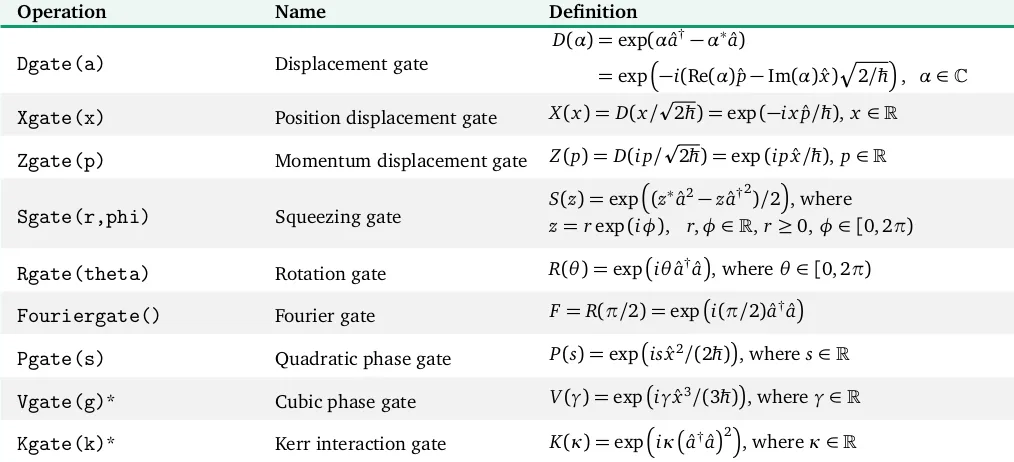
Dgate(a)

Displacement gate

D(α) =exp(αˆa†−α∗_ˆa)

=exp€−i(Re(α)ˆp₋Im(α)ˆx)Æ2/ħhŠ, α∈C

Xgate(x)

Position displacement gate X(x) =D(x/p2ħh) =exp(−i xˆp/ħh),x∈R

Zgate(p)

Momentum displacement gate Z(p) =D(i p/p2ħh) =exp(i pˆx/ħh),p∈R

Sgate(r,phi)

Squeezing gate

S(z) =exp€(z∗aˆ2−zaˆ†2)/2Š, where z=rexp(iφ), r,φ∈R,r≥0,φ∈[0, 2π)

Rgate(theta)

Rotation gate R(θ) =exp iθaˆ†aˆ, whereθ∈[0, 2π)

Fouriergate()

Fourier gate F=R(π/2) =exp i(π/2)aˆ†aˆ

Pgate(s)

Quadratic phase gate P(s) =exp isˆx2/(2ħh), wheres∈R

Vgate(g)*

Cubic phase gate V(γ) =exp iγˆx3/(3ħh), whereγ∈R

Kgate(k)*

Kerr interaction gate K(κ) =exp€iκ ˆa†ˆa2Š, where_κ∈R

Operation Name Definition

BSgate(theta,phi)

Beamsplitter

B(θ,φ) =exp θ(eiφ_aˆ

1aˆ†2−e−

iφ_aˆ† 1aˆ2)

, where the transmissivity and reflectivity amplitudes aret=cosθ,r=eiφsinθ

S2gate(r,p)

Two-mode squeezing gate S2(z) =exp z∗ˆa1aˆ2−zaˆ†1aˆ † 2

, wherez=rexp(iφ)

CXgate(s)

Controlled-X or addition gate C X(s) =exp(−isxˆ₁ˆp2/ħh),s∈R

CZgate(s)

Controlled phase shift gate C Z(s) =exp(isxˆ₁ˆx2/ħh),s∈R

CKgate(k)*

Controlled Kerr interaction gate C K(κ) =exp iκˆa₁†aˆ₁aˆ†₂ˆa₂,κ∈R

Table VII:Two-mode gate operations available in Strawberry Fields.

Operation Name Definition

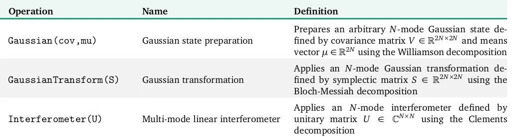
Gaussian(cov,mu)

Gaussian state preparation

Prepares an arbitrary N-mode Gaussian state de-fined by covariance matrixV _∈R2N×2N _{and means}

vectorµ∈R2Nusing the Williamson decomposition

GaussianTransform(S)

Gaussian transformation

Applies an N-mode Gaussian transformation de-fined by symplectic matrix S _{∈ R}2N×2N _{using the}

Bloch-Messiah decomposition

Interferometer(U)

Multi-mode linear interferometer

Applies an N-mode interferometer defined by unitary matrix U _{∈ C}N×N _{using the Clements}

decomposition

Table VIII:Multi-mode Gaussian decompositions available in Strawberry Fields.

Operation Name Definition

MeasureHomodyne(phi)

Homodyne measurement Projects the state onto|xφ〉〈xφ| where ˆx_φ=cosφˆx+sinφˆp

MeasureHeterodyne()

Heterodyne measurement Projects the state onto the coherent states, sam-pling from the joint Husimi distribution _π1〈α|ρ|α〉

MeasureFock()*

Photon counting Projects the state onto|n〉〈n|

Table IX:Measurement operations available in Strawberry Fields. Those indicated with an asterisk (*) are non-Gaussian and can only be used with a backend that uses the Fock representation.

Gate Decompositions

In addition, the Strawberry Fields frontend can be used to provide decompositions of certain compound gates. The following gate decompositions are currently supported.

Quadratic phase gate

The quadratic phase shift gate

Pgate(s)

is decomposed into a squeezing and a rotation,

P(s) =R(θ)S(r eiφ),

where cosh(r) = p1+ (s/2)2_{, tan(θ) = s/2, and φ =} −sign(s)π₂−θ.

Two-mode squeeze gate

The two-mode squeeze gate

S2gate(z)

is decomposed into a combination of beamsplitters and single-mode squeezers

Controlled addition gate

The controlled addition or controlled-X gate

CXgate(s)

is decomposed into a combination of beamsplitters and single-mode squeezers

C X(s) =B(φ, 0) [S(r)⊗S(−r)]B(π/2+φ, 0),

where sin(2φ) = −1/cosh(r), cos(2φ) = −tanh(r), and sinh₍r) =−s/2.

Controlled phase gate

The controlled phase shift gate

CZgate(s)

is decomposed into a controlled addition gate, with two rotation gates act-ing on the target mode,