[Wang* 5(3): March, 2018] ISSN 2349-4506
Impact Factor: 3.799
G
lobal
J
ournal of
E
ngineering
S
cience and
R
esearch
M
anagement
http: // www.gjesrm.com © Global Journal of Engineering Science and Research Management
PREDICTIVE COMPLEX EVENT PROCESSING USING EVOLVING BAYESIAN
NETWORK
HUI GAO, YONGHENG WANG*
*College of Computer Science and Electronic Engineering, Hunan University, Changsha 410082, China
DOI: 10.5281/zenodo.1204185
KEYWORDS
:
streaming big data, evolving Bayesian network, complex event processing, incremental learning, structure learning.ABSTRACT
In view of the real-time change of data distribution and poor performance of fixed models in the streaming big data environment, we propose a novel structure learning method based on evolving Bayesian network. On the basis of Minimum Description Length and Max-Min Hill-Climbing algorithm, we improve the process of model construction and take Gaussian mixture model and EM algorithm for reasoning. When learning the model structure from the event flow, our method supports incremental calculation of scoring metric, and when the data and the model do not match, it can modify the model in time and support the dynamic updating of the network structure. The experimental results show that the proposed method is superior to the traditional methods in dealing with synthetic data and real data, which is more accurate and applicable to the prediction of complex events.
INTRODUCTION
With the rapid development of Internet technology and the advent of the big data era, the data generated by applications such as e-commerce, online advertising and Weibo data is continuously accumulated and a large number of applications are being transformed into data-centric, data-intensive computing and big data analysis are gradually attracting people's attention.Big data has the characteristics of huge amount of data, high real-time requirement and low value density. Therefore, how to deal with the continuously generated data streams in real time and get more valuable information is the key point of streaming big data research.
The most important thing in dealing with streaming data is to grasp the relationship between online data streams, the less time it takes to make decision and the more valuable information you get. Most data streams consist of primitive events generated by the Internet, social networks and sensor networks. The semantic information within the primitive events is quite limited.In practice, people usually pay more attention to higher-level information such as business logic and rules. For example, traffic management systems generate huge events flow daily, but accident detection systems are only concerned with events that may lead to traffic accidents. There are many device-aware terminals in the Internet of Things, and the events that are directly obtained are called primitive events. Complex event processing (CEP) is the process of identifying top-level events by interpreting and combining the primitive event streams, and the identified top-level events are often of significant importance to the user [1]. Predictive complex event processing is to predict possible future events by monitoring and analyzing event streams.For example, in order to predict the possibility of congestion at an intersection, it can be obtained by analyzing the traffic data of the intersection, later, the vehicle navigation system can be used to guide the traffic diversion so as to reduce the congestion.
Currently, there are some challenges with predictive CEP for streaming big data.First of all, the traditional method of predictive analysis is designed for the database, which means that all the data can be obtained at any time in the process. However, the system can only process single-pass data when predicting streaming data and cannot control the sample order over time. Secondly, the data distribution in the data stream may change in real time, meaning that there is a concept drift and the fixed models learned from historical data may no longer fit the new data.Finally, the event flow often has a high incoming rate, if the model training time is too long, it will cause data backlog problems, more difficult to achieve the real-time requirements.
[Wang* 5(3): March, 2018] ISSN 2349-4506
Impact Factor: 3.799
G
lobal
J
ournal of
E
ngineering
S
cience and
R
esearch
M
anagement
RELATED WORK
There are four main ideas in CEP: Get primitive events from huge data streams; The aggregation events and correlation events are detected according to the specific patterns and rules, and meaningful events are extracted through the event operators; Proceed with the primitive events or complex events to obtain the temporal, hierarchical, causal and other semantic relationships among these events; Ensure that complex event information can be sent to users for decision making [2].The basic models for detecting complex events mainly include four types:Model based on Petri nets, model based on finite automata, model based on directed graph and model based on tree matching.As a typical directed graph model, Bayesian Network (BN) [3] adopts Directed acyclic graph (DAG) to represent complex events, has powerful modeling and inference mechanisms. Various queries and predictions are made by effectively integrating prior knowledge and current observations.
Some domestic and foreign researchers have studied the prediction analysis for many years and put forward a series of models and algorithms.Among these models, deep neural networks and Bayesian networks are widely used and they are more popular in streaming data prediction.Huang et al. proposed a method of predictive analysis based on deep belief networks, using deep belief networks at the bottom and regression models at the top to support the final prediction [4]. Predictive analysis method using deep learning model usually achieve better accuracy, but the model training is complicated and prone to over-fitting problem. As one of the well-known theoretical models in the field of reasoning, Bayesian Network has its own unique advantages in representing uncertain knowledge and is widely used in predictive analysis. Zhu et al. proposed a Bayesian network traffic flow estimation model based on a priori link flows. The model first determines the prior distribution of the variables by a priori segment flow, and then gives the posterior distribution by updating some of the observed flows. Finally, the point prediction and the corresponding probability interval are given based on the obtained posterior distribution [5].To solve the concept drift in the data stream, an evolving Bayesian network is needed. For a sudden drift, a common way to evolve Bayesian networks is to learn different models and switch between different models as the data distribution changes [6]. Li et al. proposed an incremental BN structure learning framework based on BIC metric and a new evaluation criterion ABIC (Adopt Bayesian Information Criterion), and then used a three-phase algorithm to learn BN structure [7]. Compared with this article, their method is not designed for the data stream.
As the number of possible structures of Bayesian network increases exponentially with the number of nodes, learning Bayesian network structure from data has been proved to be an NP-Hard problem. It is usually infeasible to use deterministic exact algorithms to solve the optimal network structure, so approximate algorithms and heuristic search algorithms are generally used to solve them. Approximate structure learning algorithms are usually divided into two groups, namely constraint-based approaches and search-and-score approaches. The commonly used score metrics include Bayesian Information Criterion (BIC) [8], Bayesian Dirichlet equivalent (BDe) [9] and Minimum Description Length (MDL) [10], etc.Because only the best network structure needs to be obtained in streaming data prediction, heuristic search-based methods usually find them faster, such as hill-climbing algorithm [11], simulated annealing algorithm [12], genetic algorithm [13], and so on. Based on the dependency analysis and hill-climbing algorithm, Tsamardinos et al. proposed a Max-Min Hill-Climbing (MMHC) algorithm [14], which uses the Max-Min Parents and Children (MMPC) algorithm [15] to generate candidate parent nodes, finally, the greedy search algorithm to determine the dependencies for the edges in the structure.MMHC algorithm is one of the most effective algorithms for learning Bayesian networks. Compared with the related works, our work is mainly to consider how to calculate incremental scoring metrics for streaming data and to evolve the Bayesian network model, so that the model does not need to be trained all over again.
CONSTRUCTION OF STREAMING DATA PREDICTION MODEL
Bayesian network model
A Bayesian network can be expressed as 𝐵 = (𝐺, ∅)where 𝐺 = (𝑋, 𝐴) represents a directed acyclic graph.X is a set of nodes in the network and 𝑋𝑖∈ 𝑋 is a random variable in the finite field. A corresponds to a set of directed arcs between nodes, indicating a direct dependency between variables, 𝑎𝑖𝑗 ∈ 𝐴 represents the directional connection between variables Xi and Xj, denoted Xi→Xj,node Xi is referred to as the parent node of node Xj and
[Wang* 5(3): March, 2018] ISSN 2349-4506
Impact Factor: 3.799
G
lobal
J
ournal of
E
ngineering
S
cience and
R
esearch
M
anagement
http: // www.gjesrm.com © Global Journal of Engineering Science and Research Management
distribution of node Xi given its parent node set 𝜋(𝑋𝑖). It can be seen that a Bayesian network 𝐵 = (𝐺, ∅) can uniquely determine a joint probability distribution over a set of random variables 𝑋 = {𝑋1, 𝑋2, … , 𝑋𝑛} using the graph structure and network parameters:
𝑃(𝑋1, 𝑋2, … , 𝑋𝑛) = ∏𝑛𝑖=1𝑃(𝑋𝑖|𝜋(𝑋𝑖)) (1)
The Bayesian network model structure for streaming data prediction is shown in Figure 1, where the X-axis represents the type of event and the Y-axis represents time.The type of event is related to some of the properties of the object (such as the location of the object) or to some state of the system (such as road traffic flow).Assuming a certain event type N, the state of a node (i,t) in the forecasting task is related to several groups of states (parent nodes) before time t, and the node directly connected to the node (i,t) by directed edge in Figure 1 is its parent node.Let xi,t denotes the state variable of node (i,t), pa(i,t) denotes the parent node set of (i,t),NP represents the
number of nodes in pa(i,t), NTΔt represents a time window,this means that only the nodes from time t-NTΔt to
t-Δt are considered as the parent nodes of the node at time t.The set of state variables of pa(i,t) are represented as
𝑋𝑝𝑎(𝑖,𝑡)= {𝑥𝑗,𝑠|(𝑗, 𝑠)𝜖𝑝𝑎(𝑖, 𝑡)}. According to Bayesian network theory, the joint probability distribution of all nodes in the network can be expressed as:
𝑝(𝑋) = ∏ 𝑝(𝑥𝑖,𝑡 𝑖,𝑡|𝑋𝑝𝑎(𝑖,𝑡)) (2)
The conditional probability 𝑝(𝑥𝑖,𝑡|𝑋𝑝𝑎(𝑖,𝑡)) can be calculated as:
𝑝(𝑥𝑖,𝑡|𝑋𝑝𝑎(𝑖,𝑡)) =
𝑝(𝑥𝑖,𝑡 , 𝑋𝑝𝑎(𝑖,𝑡))
𝑋𝑝𝑎(𝑖,𝑡) (3)
Since it is not easy to calculate the joint probability distribution 𝑝(𝑥𝑖,𝑡, 𝑋𝑝𝑎(𝑖,𝑡)), this article uses the Gaussian Mixture Model (GMM) [16] to approximate it like the following:
𝑝(𝑥𝑖,𝑡 , 𝑋𝑝𝑎(𝑖,𝑡)) = ∑𝑀𝑚=1𝜋𝑚𝑔𝑚(𝑥𝑖,𝑡 , 𝑋𝑝𝑎(𝑖,𝑡)|𝜇𝑚 , ∑𝑚) (4)
Where M represents the number of Gaussian models, 𝑔𝑚(· |𝜇𝑚, ∑𝑚) is the distribution of the m-th Gaussian model, 𝜇𝑚 is the mean vector, ∑𝑚 is the covariance matrix, 𝜋𝑚 is the coefficient of the m-th Gaussian model, and ∑𝑀𝑚=1𝜋𝑚= 1.Using the EM algorithm [16] we can deduce {𝜋𝑚, 𝜇𝑚, ∑𝑚}𝑚=1𝑀 from historical data, then according to the obtained parameters, the conditional distribution 𝑝(𝑥𝑖,𝑡, 𝑋𝑝𝑎(𝑖,𝑡)) can be calculated, thus, 𝑝(𝑥𝑖,𝑡|𝑋𝑝𝑎(𝑖,𝑡)) is calculated.Since the GMM parameters can be updated based on the EM algorithm, the main consideration in the research is how to evolve the structure of the Bayesian network.
Event type
ti
m
e
1 i N
t
t-Δt
t-NTΔt
···
···
···
··
· ···
Figure 1. The structure of Bayesian network model
Bayesian network structure learning
[Wang* 5(3): March, 2018] ISSN 2349-4506
Impact Factor: 3.799
G
lobal
J
ournal of
E
ngineering
S
cience and
R
esearch
M
anagement
and-score method as the scoring function of the structure.MDL is a data compression-based scoring method that is defined as follows:𝑠𝑐𝑜𝑟𝑒𝑀𝐷𝐿(𝐺: 𝐷) = ∑ log2𝑃(𝑡𝑖) + |𝐺|log2𝑚
2 𝑚
𝑖=1 , 𝑡𝑖∈ 𝐷 (5)
In the scoring function, D is the sample data set, m is the total number of samples, ti represents a sample in the
sample set D, that is, a certain row in the data set. |𝐺|=∑𝑛 2|𝜋(𝑋𝑖)|
𝑖=1 ,
|𝜋(𝑋
𝑖)|
represents the number of parents of node Xi.The Bayesian network G with the smallest score is the result, and the smaller the score, the better thematch between structure G and sample dataset D.The model with the smallest score will be used as the basis for the next search iteratively until the score does not decrease.
Since we are studying evolutionary learning of Bayesian networks, the impact of new data on the current structure needs to be considered.The current structure is based on previous data learning and needs to determine how well the current structure G matches the new data set ∆𝑡𝐷,if the matching degree is good, the current structure need not be changed and continue to wait for the incremental data to arrive, otherwise, new structures need to be learned. Let 𝜀 = |𝑠𝑐𝑜𝑟𝑒𝑀𝐷𝐿(𝐺: ∆𝑡𝐷) − 𝑠𝑐𝑜𝑟𝑒𝑀𝐷𝐿(𝐺: 𝐷)|, we set a threshold 𝛿, if 𝜀 ≤ 𝛿, indicating that the current structure is better matched to the new dataset, do not need to change the current structure. If 𝜀 > 𝛿, this indicates that the current structure is less well-matched to the new dataset and the current structure needs to be relearned.
Evolving structure learning method
At the beginning of structure learning, we need to determine the initial structure under the previous dataset. In this paper, the original Bayesian network structure is obtained through MMHC (Max-Min Hill-Climbing) algorithm [14], and the time window is used to control the amount of new data.Due to the fact that the data stream continuously generates data characteristics in actual situations, it is impossible to determine the end time of the data, so the current time is taken as the end time. When the new data set ∆𝑡𝐷 arrives, a new data set Dnew is formed in combination with the previous data set D.Judging whether the current structure matches the new dataset or not, if the matching degree is good, the current structure is already the best structure and continues to wait for the new data to arrive. Otherwise, the current structure needs to be adjusted to match new data set to achieve the best fit.Evolving structure learning algorithm as shown in Algorithm 1, each stage of the algorithm learns a new structure based on the previous structure.Among them, the third line is to determine whether the current structure and data match the basis, lines 6-10 indicate that edges are added to the structure in turn, and the structure is scored. If a lower fractional structure is obtained, the previous structure is replaced with the current one and the process is repeated until the lowest fractional structure is obtained.Similarly, lines 11-15 indicate that the edges in the structure are sequentially removed, and then the structure is scored. If a lower fractional structure is obtained, the previous structure is replaced by the current one and the process is repeated until the lowest fractional structure is obtained. Lines 16-20 indicate that the edges of existing edges are converted in turn, and then the structure is scored. If a lower fractional structure is obtained, the previous structure is replaced by the current one and the process is repeated until the lowest fractional structure is obtained. In the algorithm, add_edge (), remove_edge (), reverse_edge () all need to satisfy the DAG structure, that is, the ring structure cannot appear in the evolution of the edge.
Algorithm 1 Evolving structure learning algorithm
Input The initial structure G obtained by MMHC, initial data set D, data time window ∆𝑡𝐷, threshold 𝛿 Output The best BN structure
1 while (∆𝑡𝐷 is not none) 2 Dnew=D+∆𝑡𝐷 ;
3 ε = |scoreMDL(G: Dnew)-scoreMDL(G: D)|; 4 if (ε ≤ δ ) continue;
5 else
6 for i=1: length (G) 7 G_cur=add_edge (G);
[Wang* 5(3): March, 2018] ISSN 2349-4506
Impact Factor: 3.799
G
lobal
J
ournal of
E
ngineering
S
cience and
R
esearch
M
anagement
http: // www.gjesrm.com © Global Journal of Engineering Science and Research Management
9 if (∆𝑆 <0) G=G_cur; 10 end for
11 for i=1: length (G)
12 G_cur =remove_edge (G);
13 ∆S = scoreMDL(G_cur: Dnew)-scoreMDL(G: Dnew); 14 if (∆𝑆 <0) G=G_cur;
15 end for
16 for i=1: length (G)
17 G_cur =reverse_edge (G);
18 ∆S = scoreMDL(G_cur: Dnew)-scoreMDL(G: Dnew); 19 if (∆S <0) G=G_cur;
20 end for 21 end else 22 end while 23 return BN;
EXPERIMENT
The experiment is divided into two parts. The experimental models are analyzed respectively by the known classical Bayesian networks and real traffic data, which fully validate the validity of the evolving Bayesian network prediction model.
Predict known networks
When using the well-known Bayesian networks, the commonly used Alarm Network [17] and Pathfinder Network [18] are chosen. The parameters of the two networks are shown in Table 1 below.
Table 1. Parameters of networks
Benchmark Variables Edges Instances Av.Deg Max.Deg
Alarm 37 46 10000 2.5 6
Pathfinder 109 195 10000 1.7 106
Since this article presents an evolutionary structure learning model based on Bayesian network in streaming big data environment, Evol_BN, an evolutionary learning model, is compared with Batch_BN, a batch model based on Bayesian network to illustrate the experimental results. We analyze the impact of different time windows on the network model construction in streaming data environment. The criteria for evaluating the accuracy of structural learning methods are to extract samples from a known Bayesian network, apply structural learning methods to the data, and compare the learned structure with the original structure. Judgment is based on the structural Hamming Distance (SHD), SHD (G) = IN (G) + DE (G) + RE (G), where IN (G) denotes the number of added edges compared to the original structure,DE (G) denotes the number of edges reduced compared to the original structure, and RE (G) denotes the number of reverse edges compared to the original structure.In this experiment, the size of the time window is set at 1000, and the SHD comparison chart about the Alarm and Pathfinder networks are shown in Figure 2 and Figure 3 respectively.
[Wang* 5(3): March, 2018] ISSN 2349-4506
Impact Factor: 3.799
G
lobal
J
ournal of
E
ngineering
S
cience and
R
esearch
M
anagement
It can be seen from Figure 2 and Figure 3 that when the initial number of instances is 1000, the SHD obtained by the method of evolutionary structure learning is the same as the traditional batch method, indicating that the initial network models constructed by these two methods have the same accuracy. As the time window expands, i.e., the number of instances increases, it can be clearly seen that the evolutionary structure learning method has better model accuracy, less SDH than the batch processing method, especially the more complicated the network structure, the difference is more obvious. By comparing the experimental results, we can see that the network structure built by evolutionary Bayesian network model is closer to the real structure. It automatically adjusts the original structure in the continuous learning of the data stream, which is a dynamic optimization process, and thus closer and closer to the original network structure.Predict real data
The real data obtained from the experiment is derived from the PeMS Traffic Monitoring System (https://pems.eecs. berkeley.edu/), it is the real-time traffic data obtained by the California Department of Transportation Highway Performance Monitoring System.We selected the one-week traffic data from March 6, 2017 through March 12, 2017 for the experiment, including speed, flow, and occupancy. Speed represents the average speed of the vehicle passing the sensor over the time interval Δt. Flow represents the total number of
vehicles passing the sensor over the time interval Δt.Occupancy, as a measure of the vehicle's density, represents
the ratio of the occupancy time of the vehicle observed by the induction coil to the total observed time over the time interval Δt.As can be seen from Figure 4 and Figure 5, there is a clear dependency between the three data
sources and a clear period of peak period.
Figure 4. Flow - speed diagram Figure 5. Flow - occupancy diagram
In simple terms, the state of traffic flow in urban roads can be divided into free flow and congestion flow.Free flow describes the situation in which vehicles do not interact with each other and tend to travel at the maximum allowable speed of Vmax. On the other hand, congestion flow characterizes the increase of traffic density and the
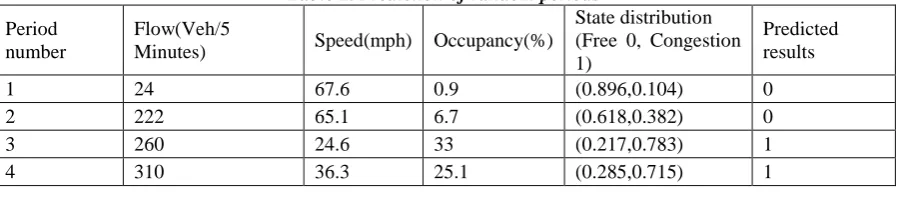
decrease of speed due to vehicle interaction.Set the time window is 5min, the three data sources of speed, flow and occupancy were considered.The evolutionary Bayesian network structure learning is applied to the research of traffic flow state prediction model, and the traffic flow state of a specific time period is predicted by combining the observations of various data sources.This method effectively overcomes the limitations of relying on a single parameter and fully embodies the process of identifying complex events (such as traffic state) from the primitive events.In the experiment, the prediction result is 0, indicating that the current time period is in a free flow state, and a prediction result of 1 indicates that the current time period is in a congestion flow state. The traffic conditions are selected randomly for 4 periods, and the prediction results are shown in Table 2.
Table 2. Prediction of random periods
Period number
Flow(Veh/5
Minutes) Speed(mph) Occupancy(%)
State distribution (Free 0, Congestion 1)
Predicted results
1 24 67.6 0.9 (0.896,0.104) 0
2 222 65.1 6.7 (0.618,0.382) 0
3 260 24.6 33 (0.217,0.783) 1
[Wang* 5(3): March, 2018] ISSN 2349-4506
Impact Factor: 3.799
G
lobal
J
ournal of
E
ngineering
S
cience and
R
esearch
M
anagement
http: // www.gjesrm.com © Global Journal of Engineering Science and Research Management
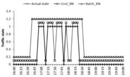
In order to verify the validity of the traffic flow state prediction model, the actual traffic state in the experiment was compared with that predicted by Evol_BN, an evolutionary structure learning method, and Batch_BN, a batch learning method.Figure 6 is a comparison chart of prediction results of time period 16: 00-20: 00.To see the difference clearly from the chart, here the results of Evol_BN are increased by 0.1, and the results of Batch_BN are increased by 0.2.In other words, the traffic state is 0/0.1/0.2 at each time period indicates the free flow state, and the traffic state is 1/1.1/1.2 indicates the congestion flow state.
Figure 6.Comparison chart of traffic state prediction results
The trend of traffic state from free flow to congestion flow can be clearly seen from the figure, and the Bayesian network model constructed by evolutionary structure learning method can get more realistic forecast results than the traditional batch method model, closer to the real traffic conditions.For example, at 17:10, the actual traffic state is free flow, the free flow is predicted by Evol_BN method, and the congestion flow is obtained by Batch_BN method.The experimental results show that the proposed method can effectively and accurately predict traffic flow state. Compared with traditional BN, it improves accuracy and can solve the prediction problem of complex flow events.
CONCLUSION
Based on the traditional Bayesian network model, this paper proposes a predictive complex event processing method using evolving Bayesian networks.Based on the time window, the incremental learning of new data is realized, the new data is more matched with the model structure, and a process for automatic adjustment of different environments is implemented, which is suitable for a complex data environment.This method is mainly to improve the structure model construction process of Bayesian network. First of all, according to the existing knowledge to learn the initial network structure, afterwards, through continuous adjustments to adapt to the new data, an optimal score is obtained, and there is a criterion for the current structure and data, so that it is not necessary to relearn each time to improve the inefficiency, finally, on the basis of the local structure, the search space is reduced through effective constraints and the complexity is reduced.This method effectively solves the problem of predicting complex events in the streaming big data environment. However, the data flow is simulated through the time window in this experiment. How to improve it to bring it closer to the real-time streaming big data environment is the focus of the next study.
ACKNOWLEDGEMENT
This project is sponsored by the "Research on Autonomous Knowledge Obtaining Technology for big streaming data (kq1706020)" project of Changsha technological plan.
REFERENCES
1. Etzion O, Niblett P. Event Processing in Action [M]. Stamford: Manning Publications Company, 2010. 2. Cao K, Wang Y, Li R, et al. A Distributed Context-Aware Complex Event Processing Method for
Internet of Things [J]. Journal of Computer Research & Development, 2013, 50(6):1163-1176.
[Wang* 5(3): March, 2018] ISSN 2349-4506
Impact Factor: 3.799
G
lobal
J
ournal of
E
ngineering
S
cience and
R
esearch
M
anagement
4. Huang W, Song G, Hong H, et al. Deep Architecture for Traffic Flow Prediction: Deep Belief NetworksWith Multitask Learning [J]. IEEE Transactions on Intelligent Transportation Systems, 2014, 15(5):2191-2201.
5. Zhu S, Cheng L, Chu Z. A Bayesian network model for traffic flow estimation using prior link flows [J]. Journal of Southeast University, 2013, 29(3):322-327.
6. Pascale A, Nicoli M. Adaptive Bayesian network for traffic flow prediction [C]//Statistical Signal Processing Workshop. IEEE, 2011:177-180.
7. Li S, Zhang J, Sun B, et al. An Incremental Structure Learning Approach for Bayesian Network [C]//Control and Decision Conference. IEEE, 2014:4817-4822.
8. Schwarz G. Estimating the Dimension of a Model [J]. Annals of Statistics, 1978, 6(2):15-18.
9. Cooper G F, Herskovits E. A Bayesian Method for the Induction of Probabilistic Networks from Data [J]. Machine Learning. 1992, 9(4):309-347.
10. Rissanen J. A universal prior for integers and estimation by minimum description length [J]. The Annals of Statistics, 1983, 11(2):416-431.
11. Gámez J A, Mateo J L, Puerta J M. Learning Bayesian networks by hill climbing: efficient methods based on progressive restriction of the neighborhood [J]. Data Mining & Knowledge Discovery, 2011, 22(1-2):106-148.
12. Ye S, Cai H, Sun R. An Algorithm for Bayesian Networks Structure Learning Based on Simulated Annealing with MDL Restriction [C]//International Conference on Natural Computation. IEEE Computer Society, 2008:72-76.
13. Xiufeng W, Yimei R. Learning Bayesian networks using genetic algorithm [J]. Journal of Systems Engineering & Electronics, 2012, 18(1):142-147.
14. Tsamardinos I, Brown L E, Aliferis C F. The max-min hill-climbing Bayesian network structure learning algorithm [J]. Machine Learning, 2006, 65(1):31−78.
15. Tsamardinos I, Aliferis C F, Statnikov A. Time and sample efficient discovery of Markov blankets and direct causal relations [C]//In: Proceedings of the 9th ACM SIGKDD International Conference on Knowledge Discovery and Data Mining. New York, USA: ACM, 2003. 673-678.
16. Bishop, C.M.: Pattern Recognition and Machine Learning [M]. New York: Springer, 2006.
17. Beinlich I A, Suermondt H J, Chavez R M, et al. The ALARM Monitoring System: A Case Study with two Probabilistic Inference Techniques for Belief Networks [M]. Springer Berlin Heidelberg, 1989:247-256.