A Novel Concise Adaptive Neural Control for a
Class of Nonlinear MIMO Systems with
Unknown Time Delays
Guoqing Zhang, Xianku Zhang and Guoping Xu
Navigation College, Dalian Maritime University, Dalian, Liaoning, 116026, China Email: [email protected], [email protected], [email protected]
Abstract—This note makes effort at the problem of robust adaptive control for a class of nonlinear MIMO systems with unknown time-delays. A concise adaptive neural control scheme is developed by using the Backstepping method, the Lyapunov-Krasovskii functional and a novel “MLN” technique. Unlike the existing literatures, the actual control laws are only composed of the state variables, the reference signals and their derivatives, independent of the designed virtual controls and the other intermediate variables. In addition, only n (the number of system outputs) neural networks are introduced to compensate the nonlinear uncertainties of the whole system. Thus, the outstanding advantage of the proposed scheme is that the control law with a concise structure is model-independent and easy to implement in practical engineering, due to less computational burden. The corresponding scheme guarantees uniform ultimate boundedness of all the signals in the closed-loop system, and the tracking errors can converge to a arbitrary small neighborhood of zero. Finally, a simulation example illustrates the effectiveness of the proposed scheme.
Index Terms—robust adaptive control, neural networks, MIMO systems, time delays
I. INTRODUCTION
Recently, the development of adaptive neural control algorithms for uncertain nonlinear systems has been a focus of engineering interest as well as theoretical significance. Many positive results have shown that semi-global uniform ultimate boundedness (SGUUB) of the closed-loop adaptive control system can be achieved and the output of the system is proven to converge to a small neighborhood of the desired trajectory, refer to [1-3] and the references therein for details. In [4], direct adaptive neural network (NN) control was proposed for a class of affine nonlinear systems with unknown nonlinearities. The scheme could avoid the controller singularity problem completely, by using a special property of the affine term. With the help of the Lyapunov-Krasovskii thermo, the control scheme was extended to control uncertain nonlinear systems with unknown time delays [5]. The extensively significant results on adaptive neural control also have been reported in [6, 7].
For multi-input multi-output (MIMO) nonlinear systems, the control task is very difficult due to the state
and input interconnections among various subsystems, which often severely limits system performance, even leading instability. Therefore, there exist relatively few research results available for nonlinear MIMO systems [8-10], comparing with the vast amount of results on control design for single-input, single-output (SISO) systems. In these results, the tracking control of nonlinear MIMO systems was addressed. Unlike the other literatures, this algorithm introduced NNs to approximate and compensate for both unknown functions and the uncertain time-delay function bounds, and simulation results have illustrated the effectness of the corresponding scheme. However, the aforementioned algorithm suffered from two major problems as expounded in [11]: the first one is the well known “explosion of complexity”, which is inherent in the conventional backstepping technique [12]. It is caused by the repeated differentiations of virtual controls, which is impossible to implement in practice and leads to a complicated algorithm with heavy computational burden, especially for the high-order nonlinear system. The second problem is the so-called “curse of dimensionality”, i.e., to satisfy the approximation requirement of high-order uncertain nonlinear system, the number of NNs and that of parameters to be updated online in the previous adaptive schemes is very large. In order to solve these problems, the dynamic surface control (DSC) technique [6, 13] and the minimal learning parameters (MLP) algorithm [14, 15] were extended to NNs-based adaptive control for nonlinear MIMO system in [16-18].
for a class of nonlinear MIMO systems with unknown time delays. The nonlinear uncertainties and unknown state time delays at each step are delivered to the next step, without being compensated as in the conventional adaptive neural control. In the sequel, the uncertainties of the whole system are dealt with by introducing a radial-basis-function (RBF) NNs in the final step.
The main contributions of this note can be summarized as follows: 1) In the proposed scheme, the problems of “explosion of complexity” and “curse of dimensionality” are solved from the root causes, different from DSC and MLP. The number of online learning NNs is reduced to
only n, which is equal to the number of the systems outs
and independent of the system orders. The intermediate controls would not appear in the control scheme. That will lead to a much simpler controller with less computational burden. 2) The adaptive law proposed in this note is merely dependent on the state variables, the reference signals and their mth order derivatives. With the special property and structure of our algorithm, the potential controller singularity problem existing in may adaptive control algorithm is avoided.
II. PROBLEM FORMULATION
In this note, we solve the adaptive control problem of the following nonlinear MIMO system with unknown time delays.
, , , , , , 1 , ,
, , 1 , 1 ,
,1
( ) ( ) ( ),
1, 2, , 1
( , ) ( , ) ( )
, 1, 2, ,
j j j j j j j j
j j j j
j i j i j i j i j i j i j i j i
j j
j m j m j j m j j j m j j
x f x g x x h x
i m
x f X u g X u u h X
y x j n
τ
τ +
− −
= + +
⎧ ⎪
= −
⎪
⎨ = + +
⎪
⎪ = =
⎩
"
"
(1)
where, T T T
1
[ , , ] n m n
X= x " x ∈R× with xj=[xj,1, ", xj m, j]T
denotes the matrix of state variables, T
1
[ , , ] n n
y= y " y ∈R is
the system output. T
,j [ ,1, , ,j] j i j i j j i
x = x " x ∈R , uj=[ ,u1"uj]T . ,j ,j( ,j)
j i j i j i
xτ =x t−τ with τjijas unknown time delays of the
states. T
,j [ ,1, , ,j] j i j j i
xτ = xτ " xτ , 1
T T T
1, ,
[ , , ]
n m n m
Xτ = xτ " xτ are the vector of delayed state variables. fj i,j( )⋅ ,gj i,j( )⋅ and hj i,j( )⋅
are all unknown nonlinear continuous functions. For
,
[ , 0]
j j i
t∈ −τ , xj i,j( )t are assumed to be smooth and bounded.
Remark1: Comparing with [9], e.g. the control gain
function gj m,j( )⋅ includes all state variables and the inputs
of the previous subsystems. Obviously, the plant (1) describes a class of nonlinear MIMO systems with more general form.
The following assumptions on system (1) are introduced.
Assumption1: The unknown virtual control gain
functions are confined within a certain range such that
, ,
0 ( )
j j
j j i j i
g g g
< ≤ ⋅ ≤ < ∞ (2)
where gj and gj i,j are the positive constant lower and
upper bound parameters.
Remark2: Assumption is reasonable for gj i,j( )⋅ being
away from zero is the controllable condition of (1), which is made in current literatures. It should be mentioned that
j
g and gj i,jare only required for analytical purpose, which
is not necessarily known in the proposed scheme.
Assumption2: The reference signals ydj( ), t j=1, ,"n and
their time derivatives up to the mjth order are continuous
and bounded.
Assumption3: The unknown smooth function hj i,j(xτj i,j)
satisfies the following inequality:
,
, , , ,
1
( ) j j( ) j j
i j i j i j i j l j l
l
h xτ Q xτ
=
≤
∑
(3)where ,
,j( ) j i j l
Q ⋅ are the positive functions for l=1, ",ij.
The control objective is to develop a novel concise adaptive neural tracking controller such that 1) all states of the uncertain nonlinear MIMO system (1) are SGUUB,
and 2) the tracking error zj=yj−ydj can be rendered
arbitrary small.
In this note, RBF NNs are introduced to compensate all the systems uncertainties. As pointed out in [9, 16], universal approximation results indicate that, given a
desired level of accuracy δ, approximation to that level
of accuracy can be guaranteed by making l sufficiently
large. Therefore, the NNs T ( )
W S Z can approximate any
given real continuous function f Z( ) with f(0) 0= , which
is written as (4).
T
( ) ( ) ( ), Z q Z
f Z =W S Z +δ Z ∀ ∈Ω ⊂R (4)
where, l>1is the number of the NN nodes. δ( )Z is the
approximation error with unknown upper bound
δ . T
1 2 [ , , , ]l
W=w w "w is the weight vector, T
1 2
( ) [ ( ), ( ), , ( )]l
S Z =s Z s Z "s Z is a vector of RBF basic
functions with the form of Gaussian functions defined by
(5). T
,1 ,2 ,
[ , , , ]
i i i i q
μ = μ μ "μ is the center of the receptive fields,
η is the width of the Gaussian function, and ζ is gain
coefficient.
T 2
( ) ( )
( ) exp , 1,2, ,
2
i i
i
Z Z
s Z ζ μ μ i l
η
⎡ − − ⎤
= ⎢− ⎥ =
⎣ ⎦ " (5)
In order to design the novel adaptive law, Lemma1 will be explored.
Lemma1: [19, 20] Consider the RBF NNs described in
(4), let : 1min
2 i j i j
φ = ≠ μ μ− . Then one may take an upper
bound of S Z( ) as (6).
1 2 2 *
0
( ) 3 ( 2)q exp( 2 ) : k
S Z q k φ k η S
∞
−
=
≤
∑
+ − = (6)The limited value S* is independent of Z andl.
III. DESIGN OF CONCISE ADAPTIVE NEURAL CONTROL
In this section, we develop a concise adaptive neural controller for uncertain nonlinear MIMO system (1) with Assumptions 1-3. The backstepping design procedure
contains ( , ),j mj j=1, ,"n steps. At each step, the
Lyapunov- Krasovskii functional is constructed to compensate for the unknown time delays, and the
nonlinear functions Fj i,( )⋅ and Fj i,( )⋅ shall be induced to
described the nonlinear uncertainties, which is component
the next step. In the j m, jstep, the RBF NNs is exploited
to approximate the uncertainties of the whole jth
subsystem, and the actual control ujis derived.
To illustrate the design synthesis, the notion (7) is useful, with the properties of relationship as (8).
1 2 1 2
, , , ,
1
( ), 1, 2, , ,
p p
j
i p j l j l j l l l l i
K k k k l i p i
≤ < < ≤
=
∑
= ≤"
" " (7)
1,1 , ,1
1, , 1, 1 ,
, 1, 1 ,
j j
i j i i
j j j
i p j i i p i p
j j
j i i i i i
K k K
K k K K
k K K
− − − − − − ⎧ + = ⎪⎪ + = ⎨ ⎪ = ⎪⎩ (8)
Throughout this note, ⋅ is Euclidean norm of a vector;
max( )
λ ⋅ denotes the largest eigenvalue of a square matrix.
( )ˆ⋅ is the estimate of ( )⋅ , and the estimate error ( ) ( ) ( )⋅ = ⋅ − ⋅ˆ .
For notation simplicity, let fj i, =fj i,( ),⋅ gj i, =gj i,( ),⋅
, ,( ) j i j i
h =h ⋅ where j=1, , , 1, ,"n i= "mj.
A. Controller Design
The following coordinate transformation (9) is useful to design concise adaptive laws.
,1 ,1
, , ,
, 1, 2, , , 1, 2,,
j j dj
j j i j i j i
z x y
j n i m
z x α
= −
⎧⎪ = =
⎨ = −
⎪⎩ " (9)
Furthermore, αj i, is the intermediate control laws at
each step and is chosen as follows:
,2 ,1 ,1 ,1 ,1
1
( ) ( ) ( 1)
, 1 , , 1, , 1 , ,
1
( , )
[ ] ( , )
j j j dj j j dj i
i j i p i
j i j i j i dj i p j i p dj j i j i dj p
k z y F x y
k z y K x y F x y
α α − − − + − + − = = − + − ⎧ ⎪ ⎨ = − + − − − ⎪ ⎩
∑
(10)where, kj i, >0 are design parameters, 1,
j i p
K− have been
defined in (7). Fj i,( )⋅ denotes the previous i nonlinear
uncertainties of the jth subsystem, which will be specified in each step.
Using the similar operation, the desired control laws *
j u
are derived.
1
( ) ( ) ( 1)
*
, , 1, , 1 , ,
1
[ ] ( , )
j
j j j
j j j j j
m
m j m p m
j j i j m dj m p j m p dj j m j m dj p
u k z y K x y F x y
− − − − + − = = − + −
∑
− − (11)Step (j, 1 (1 ≤ j ≤ n)). For the first differential equation of
the jth subsystem, one has
,1 ,1( ,1) ,1( ,1) ,2 ,1( ,1)
j j j j j j j j dj
z =f x +g x x +h xτ −y
(12)
With Assumption 3, completing the square gives
2 ,1 2
,1 ,1 ,1 ,1 ,1 ,1
1 1
( ) [ ( )]
2 2
j
j j j j j j
z h xτ ≤ z + Q xτ (13)
To deal with the delay term in (12), consider the Lyapunov-Krasovskii functional as follows (14).
2
,1 ,1 ,1
1 2
j j Uj
V = z +V (14)
with
,1
2 ,1
,1 ,1
1 ( ( )) d 2 j t j Uj j t
V τ Q x s s
− ⎡ ⎤
=
∫
⎣ ⎦Take time derivative of (14) alone (12), (13), it is easy to obtain (15).
,1 2
,1 ,1 ,1 ,1 ,1 ,2 ,1 ,1 ,2 ,1 ,1
,1 2
,1 ,1 ,1 ,1 ,1 ,1 ,1 ,2 ,1
,1
1 1
( ) [ ( )]
2 2
( ( ) ) [1 2 tan ( )]
j
j j j dj j j j j j j j j
j
j j j dj j j j j j j
j
V z f y z g z g z Q x
z
z g F y g z g z U
α α η ≤ − + + + + ≤ ⋅ − + + + − (15)
where, Fj,1( )⋅ is defined in (16),
,1 2
,1 ,1 ,1
1
[ ( )] 2
j
j j j
U = Q x . As
pointed out in (8), 1tanh ( )2 z
z η is well defined at z=0and
can be approximated by a RBF NNs.
,1
1 2
,1 ,1 ,1 ,1 ,1
,1 ,1
2 1
( ) ( )[ tanh ( ) ]
2 j
j j j j j
j j
z
F g x f z
z η
−
⋅ = + + (16)
Thus, substituting (10) into (15) results in
2 2 2
,1 ,1 ,1 ,1 ,1 ,1 ,2
,1 2
,1 ,1
1
[ ( 1) ]
4
[1 2 tanh ( )]
j j j j dj j j j j
j j j
V k g g y z z g z
z U η ≤ − − − + + + − (17)
The second error variable z2shall be presented.
,2 ,2 1,1( ,1 ) ,1( )
j
j j dj j dj j
z =x −y +K x −y +F ⋅ (18)
where Fj,1( )⋅ =Fj,1(xj,1, )ydj .
Step (j, i (for i=2, …, mj-1)). A similar procedure is
employed recursively for each step (j, i). The (i)th error
variable zj i, is
1
( 1) ( 1 )
, , 1, , , 1
1
[ ] ( )
i
i j i p
j i j i dj i p j i p dj j i p
z x y K x y
−
− − −
− − −
=
= − +
∑
− +F ⋅ (19)where, ( 2)
, 1( ) , 1( , 1, ) i j i j i xj i ydj
−
− ⋅ = − −
F F is constructed to represent
the nonlinear uncertainties of the previous (j,i-1) differential equations.
Using (1), then the derivative of zj i, is
1
( ) ( )
, , , , +1 1, , , 1
1
1 2
, 1 , 1 ( )
, , , 1 ( )
1 , 0
1
, 1
, 1, , ,
1 ,
[ ]
( )
i
i j i p
j i j i j i j i dj i p j i p j i p i p dj p
i i
j i j i p
j p j p j p p dj
p j p p dj
i
j i j
j i i p j i p j p
p j p
z f g x y K f g x y
f g x y
x y
h K h h
x − − − − − + − = − − − − + = = − − − − = = + − + + − ∂ ∂ + + + ∂ ∂ ∂ + + + ∂
∑
∑
∑
∑
F F F 1 1 i p − =∑
(20)With Assumption 3, the inequalities (21) can be obtained.
2 , 2
, , , , , ,
1 1
1 1
, 1
, 1, , , ,
1 1 ,
1 1 1
, 1
2 2 2 2 , 2
, 1, , , ,
1 1 1 1 , 1 1
1 1
( ) [ ( )] 2 2
1 [ ] 1 [ ] [ ( )]
2 2
i i
j i j i j i j i j i j k j k
k k
i i
j i j
j i i p j i p j i j p
p p j p
p p p
i i i
j i
j j p
j i i p j i j k j k
p k p k j p p k
z h x z Q x
z K h z h
x
z K z Q x
x τ τ τ = = − − − − − = = − − − − − = = = = = = ≤ + ∂ + ∂ ∂ ≤ + + ∂
∑
∑
∑
∑
∑∑
∑∑
∑∑
F F (21)Consider the Lyapunov-Krasovskii functional (22), whose time derivative alone (10), (20), (23) is derived in (24).
2
, , ,
1 2 j i j i Uj i
V = z +V (22)
with , , 1 2 2 , , , , ,
1 1 1
1 ( ( )) d ( ( )) d
2
j k j k
p
i t i t
j i j p
Uj i j k j k
t t
k p k
V τ Q x s s τ Q x s s
− − − = = = ⎡ ⎤ ⎡ ⎤ =
∑
∫
⎣ ⎦ +∑∑
∫
⎣ ⎦ 1 2 2 , , , , , , , ,1 1 1
1 ( ) ( ) 2
p
i i
j i j p
Uj i j i j k j k j k j k
k p k
V U Q xτ Q xτ
−
= = =
⎡ ⎤ ⎡ ⎤
= −
∑
⎣ ⎦ −∑∑
⎣ ⎦(23)
where, , 2 1 , 2
, , , , ,
1 1 1
1 ( ) + ( ) 2
p
i i
j i j p
j i j k j k j k j k
k p k
U Q x Q x
− = = = ⎡ ⎤ ⎡ ⎤ =
∑
⎣ ⎦∑∑
⎣ ⎦ . 1 ( ) ( ), ,1 , , , 1 1, , , , 1
1
1 2
, 1 , 1 ( )
, , , 1 ( )
1 , 0
( )
( )
i
i j i p
j i j j i j i j i dj i p j i p j i p j i p dj p
i i
j i j i l
j p j p j p p dj
p j p p dj
V z f g y K f g x y
f g x y
1 1
, 1
2 2
, , 1, ,
1 1 1 1 1 ,
1
2 2
, ,
, , , 1 , , , ,
1 1 1
( ) (
,1 , , , 1, , 1
1 1 1
( ) ( )
2 2 2
1
( ) ( ) 2
( ) (
p p
i i i
j i j
j i j i i p j i
k p k p k j p
p
i i
j i j p
j i j i j i j k j k j k j k
k p k
i j
j j i j i dj j i i p j i p dj
z z K z
x
z g z Q x Q x
z g F y g K x y
− − − − = = = = = − + = = = − + − ⎤ ∂ + + + ∂ ⎥ ⎥⎦ ⎡ ⎤ ⎡ ⎤ + + ⎣ ⎦ − ⎣ ⎦ ≤ ⋅ − + −
∑
∑∑
∑∑
∑
∑∑
F 1 ), , 1 1
, 2
, , , 1 ,
,
) [1 2 tanh ( )]
i
i p
j i j i p
j i j i j i j i j i
j i
g z
z g z U
α η − − + = + ⎡ ⎤ + ⎢ ⎥ ⎣ ⎦ + + −
∑
(24)where, ( 1)
,( ) ,( ,, ) i j i j i j i dj
F ⋅ =F x y − is defined in (25).
1
1 ( )
, , , 1, , , , 1
1
, 1 ( )
, , 1 , , , 1
,
2 1
, 1 ( ) 2
, , 1,
( )
0 1 1 1
( ) ( ) ( ) 1 1 [ ] 2 2 1 i
j i p
j i j i j i i p j i p j i p j i p dj p
j i i l
j i j i l dj j p j p j p j p
p
i i i
j i p j
dj j i j i i p
p
p dj k p k
F g f K f g x y
g x y f g x
x
y z z K
y − − − − − − + − = − − + − + − − − − = = = = ⎧⎪ ⎡ ⋅ = ⎨⎪⎩ + ⎣ + − ⎤ ∂ − − + ∂ + ⎥ ⎥⎦ ∂ + + + ∂ +
∑
∑
∑
∑∑
F F 1, 12 2 ,
, ,
1 1 , , ,
2
[ ] tanh ( ) 2
p i
j i j i
j i j i
p k j p j i j i
z
z U
x z η
− − = = ⎫ ∂ ⎪ + ⎬ ∂ ⎪⎭
∑∑
F (25)Substituting (10) into (25), the inequality below can be obtained easily.
2 ( )2 2
, , , , , , , 1
, 2
, ,
1 [ ( 1) ]
4 [1 2 tanh ( )]
i
j i j i j j i dj j i j i j i j i j i
j i j i
V k g g y z z g z
z U η + ≤ − − − + + + − (26)
Now, considering (8) derives the following (27), which is very useful for the design procedure.
1
( 1) ( 1 )
, , , 1, ,
1 1
( ) 1, , 1 1
( 1) ( 1)
,1 , , 1, 1 ,1 1,1 ,
( 1
, 1, 1, 1 ,
( ) [ ]
[ ]
( ) ( ) ( ) [( )(
i
i j i p
j i j i dj j i i p j i p dj p
i
j i p
i p j i p dj p
j i j j i
i j i dj j i i i j dj i j i dj
j j i
j i i p i p j i p dj
k x y k K x y
K x y
K x y k K x y K x y
k K K x y
− − − − − − = − − − + − = − − − − − − − − − + − − + − + − = − + − + − + + −
∑
∑
2 ) 1 )] i p p − =∑
( ) , , 1 1[ ( )]
i
j i p
i p j i p dj p
K x + − y −
=
=
∑
− (27)It follows from (9), (10), (19) and (27) that
( ) , 1 , 1
1
( 1) ( 1 )
, , 1, , , 1
1 1
( )
1, , 1 ,
1
( ) ( )
, 1 , , 1 ,
1
[ ( ) ( )] ( ) ( )
[ ] ( )
i j i j i kj
i
i j i p
j i j i dj i p j i p dj j i p
i
j i p
i p j i p dj j i p
i
i j i p
j i dj i p j i p dj j i p
z x y
k x y K x y
K x y F
x y K x y
+ + − − − − − − − = − − − + − = − + + − = = − + − + − + ⋅ + − + ⋅ = − + − + ⋅
∑
∑
∑
F F (28)where ( 1)
,( ) ,( ,, ) , , 1( ) ,( ) i
j i j i xj i ydj kj i j i Fj i
−
−
⋅ = = ⋅ + ⋅
F F F .
Step (j, mj). In this step, the desired actual control (11) is
firstly derived by the similar operation in step (j, i), then a RBF NNs is induced to compensate the sum of the unknown nonlinear terms.
Different from the step (j, i), the unknown functions
, j( ), ( ), ( ), j , j j m j m j m
f ⋅ g ⋅ h ⋅ contain all state variables and the
inputs of the previous subsystems. Thus, we select the
Lyapunov-Krasovskii functional 2
, , ,
1 2
j j j
j m j m Uj m
V = z +V . Using
the desired actual control (11), the corresponding time derivative is
( )
2 2 2
, , , , , 2 , , 1
[ ( 1) ]
4
[1 2 tanh ( )] j
j j j j
j j j
m j m j m j j m dj j m
j m j m j m
V k g g y z
z U η ≤ − − − + + − (29) with 1 2 2 , , , , , , ,
1 1 1 1
1 ( ) + ( )
2
j j
j j
m m p
n
j m j p
j m j k j k j k j k
j k p k
U Q x Q x
−
= = = =
⎡ ⎤ ⎡ ⎤
=
∑∑
⎣ ⎦∑ ∑
⎣ ⎦, j( ) j m
F ⋅ is constructed as (30)
1
( )
1
, , , 1, , , , 1
1
, 1 ( )
, , 1 , , , 1
, 2
, 1 ( )
, ,
( )
0 1 1
( ) ( ) ( ) 1 1 [ 2 2 j j
j j j j j j j
j j j j j j j j j m m p j
j m j m j m m p j m p j m p j m p dj p
j m m l
j m j m l dj j p j p j p j p
m n m
j m p
dj j m j m
p
p dj j k
F g f K f g x y
g x y f g x
x
y z z
y − − − − − − + − = − − + − + − − = = = ⎧⎪ ⎡ ⋅ = ⎨ + ⎣ + − ⎪⎩ ∂ ⎤ − − + ∂ + ⎥ ⎥⎦ ∂ + + + ∂
∑
∑
∑∑
F F 1 2 1, 1 1 1, 1 2 2 ,
, ,
1 1 , , ,
] 1 [ ] 2 tanh ( )
2 j j j j j j j j j m p j m p p k m p
j m j m
j m j m
p k j p j m j m
K z
z U
x z η
− − = = − − = = ⎫ ∂ ⎪ + ∂ + ⎬ ⎪⎭
∑ ∑
∑ ∑
F(30)
Substituting zj m, j =xj m, j−αj m, j into (11), we obtain (31)
by (27).
( ) ( )
*
, , 1 ,
1
[ ] ( )
j
j j
j j j
m
m j m p
j dj m p j m p dj j m p
u y K x + − y −
=
= −
∑
− −F ⋅ (31)According to (4) and Lemma1, a RBF NNs Fˆj m, j( )⋅
with input vector T T ( 1)T T ( 1 ) 1
1
[ , , mj ] n m j mj
j j dj
Z = X u− y − ∈Ω × + − + × , where
(n m j× + − +1mj) 1×
Ω is a compact set, is introduced to approximate
the Fj m, j( )⋅ with Wj being ideal constant weights.
Considering Lemma1, we choose the following actual control law (32), the weights online learning law is designed as (33).
( ) ( ) T
, , 1
1 ˆ [ ] ( ) j j j j j m
m j m p
j dj m p j m p dj j j j p
u y K x + − y − W S Z
=
= −
∑
− − (32)ˆ [ ( ) ˆ]
j j j j j j
W = Γ S Z −σW (33)
where T 0
j j
Γ = Γ > , σ >j 0are the design matrixes.
C. Stability Analysis
In this section, we state the main result in this note as follows.
Theorem1. Consider the closed-loop system consisting
of the nonlinear MIMO time-delay system (1) satisfying Assumption 1-3, the controller (32) and the concise adaptive law (33). For all initial conditions satisfying
T 1
, ,
1 1 1
1 + 2 2 j j m n n
j i j m j j j
j i j
V g W −W
= = =
Γ ≤ Δ
∑∑
∑
, with any Δ >0 , one cantune the controller parameters kj,1,"kj m, j, Γj andσj such
that all the signals in the system are semi-global uniformly ultimately bounded (SGUUB).
Proof: Consider the following Lyapunov function candidate.
2 T 1
, , ,
1 1 1
1 1 ( )+ 2 2 j j m n n
j i Uj i j m j j j
j i j
V z V g W −W
= = =
=
∑∑
+∑
Γ (34)2 2
, , , 1 , , , , 1
2
2 2
, , , ,
T T
, , ,1 ,
,
*2 2 *2 2 T
, , , ,1
1 , 4
, 4 ( ) ( )
2
j j j j
j j j
j j j j
j i j i j i j i j i j i j i j j j m j m j m j m
j j j j m j m j j j j j m j m j m j j m j m j j j j
z g z g z g z
z g g z
W S Z z g W S Z z g
g
g S z g S z W W
δ δ
+ ≤ + +
≤ +
− +
≤ + +
(35)
Based on (17), (26), (29), and (35), the time derivative of (34) is
2 2 *2 2
,1 ,1 ,1 , ,1
1 1
,
2 ( )2 2
, , ,
1 2
, ( )2
2 *2 2 2
, , , , ,1
1
, T
1
[ ( 1) ]
5
[ ( 1) ]
4
[ ( 1) ]
4
( ) (
2 2 4
j j
j j
j j j j
j n
j j j dj j j m j j j
m n
j i i
j i j j i dj j i j i
n
j m m
j m j j m dj j m j j m j
j n
j m
j j j
j j j
V k g g y g g S z
g
k g g y z
g
k g g y g S g z
g
g m
W W
σ δ
= −
= =
=
=
≤ − − − − −
− − − −
− − − − − −
− − + +
∑
∑ ∑
∑
∑
2
, 2
1 , 2
,
1 1 ,
)
4 2
[1 2 tanh ( )]
j j
n
j j m j j
m n
j i j i
j i j i
g W z
U
σ
η
=
= =
+
+ −
∑
∑∑
(36)
Letting,
1 2 2 *2
,1 0 ,1 ,1 ,
,
1 2 ( )2
, 0 ,
[ ( 1) ],
5
[ ( 1) ],
4 j
j j j j dj j j m j
j i i j i j j j i dj
k g g y g g S
g
k g g y
α
α
−
−
= + − + +
= + − +
{ }
, ( )2
1 2 *2 2
, 0 , , ,
2
, 2
,0 1
max 1
1
[ ( 1) ]
4 1
min 2 , ,
( ) 4 4 2
min , =
j j
j j j j
j j m
m
j m j j j m dj j m j j m
j j m
j j j
j j j
j n
j j
j n
j
g
k g g y g S g
g m
W
α
σ
σ δ
α α ε
λ
α α ε ε
−
−
≤ ≤ =
= + − + + +
⎧ − ⎫
⎪ ⎪
= ⎨ Γ ⎬ = + +
⎪ ⎪
⎩ ⎭
=
∑
with αj0being positive constant, (36) finally becomes
, 2
,
1 1 ,
[1 2 tanh ( )] j
m n
j i j i
j i j i
z
V αV ε U
η
= =
≤ − + +
∑∑
−(37)
Thus, by (37) the SGUUB stability follows immediately from the same line used in the proof of Theorem1 in [9, 16]. The proof is completed.
Remark3: It can be observed from (32) and (33) that the
proposed control scheme is concise and with less computational burden. Different from the current literatures, the actual control law and the adaptive law are constructed only by the state variables, the reference signals and their derivatives, independent of the designed virtual control and the other intermediate variables. Only n(equal to the number of system outputs) neural networks are introduced to compensate for the sum of all the uncertainties, regardless of the number of system orders. Thus, the problems “explosion of complexity” and “curse of dimensionality” are circumvented from the root causes. That is a novel “minimum learning networks (MLN)” technique.
IV. SIMULATION EXAMPLE
In this section, a simulation example is presented to illustrate the effectiveness of the proposed control scheme. For comparison, we consider the following uncertain nonlinear MIMO time-delay system, which has been employed in [16].
2 2
1,1 1,1 1,1 1,2 1,1
1,2 1,1 1,2 2,1 2,2
2 2
1,1 2,2 1 1,2
2,1 2,1 2,2 2,1 2,2 1,2 2,1 2,2 1,1 1
2
1 2,1 2,2 1,1 2 1,1 2,2
(1 sin ( ))
(1 sin ( ) 0.5cos ( ))
( )
(2 sin ( ) sin( ))
x x x x x
x x x x x
x x u x
x x x x
x x x x x u
u x x x u x x
τ
τ
τ
τ τ
⎧ = − + + +
⎪
= + +
⎪
⎪ + + + +
⎪
⎨ = − + +
= + −
+ + − − +
⎩
⎪ ⎪ ⎪ ⎪
(38)
where xτj i, =xj i,(t−τj i,) , for j=1, 2, 1,2i= , and
1,1 2, 1.5, 0.5, 11,2 1,2 1,2
τ = τ = τ = τ = .
The reference signals are assumed to be (39). In the
simulation, letting the signals ( )i, 0,1,2
dj
y i= pass through a
first order tilter ( )i ( )i ( )i, 5t
iyrj yrj ydj i e
τ + = τ = − +0.001, the ( )i rj
y is for
the control design.
1 2
( ) 0.5(sin( ) sin(0.5 )), ( ) 0.5sin( ) sin(0.5 ) d
d
y t t t
y t t t
= +
= + (39)
According to the control scheme in this note, the concise adaptive neural controller and the adaptive laws are as follows.
T
1 1 1,1 1,2 1,2 1 1,1 1,2 1,1 1 1 1 1
T
2 2 2,1 2,2 2,2 2 2,1 2,2 2,1 2 2 2 2
T
1 1 1 1 1,1 1 1 1 1 1
2 2 2 2 2,1 2 2
ˆ
( )( ) ( ) ( )
ˆ
( )( ) ( ) ( )
ˆ ( ) ˆ , [ , , ]
ˆ ( ) ˆ ,
r r r
r r r
r r
u y k k x y k k x y W S Z
u y k k x y k k x y W S Z
W S Z z W Z X y y
W S Z z W
σ
σ
= − + − − − −
= − + − − − −
⎡ ⎤
= Γ ⎣ − ⎦ =
⎡ ⎤
= Γ ⎣ − ⎦
T
2 [ , ,1 r1, r1] Z = X u y y
(40)
In this simulation, the initial condition is
1,1( ) 0.5, ( ) 0.1, ( ) 0.3, ( )0 1,2 0 2,1 0 2,2 0 0.15
x t = x t = x t = x t = − . The
corresponding control parameters are taken as
1,1 1,2 30, 20, 2,1 2,2 1 diag{1.0}, 2 diag{0.5},
k =k = k =k = Γ = Γ =
1 0.5, 0.22
σ = σ = . The RBF NNs in (40) includes 25 nodes,
with centers μp spaced in
6 [ 2.5, 2.5]− × for
1
u and
7 [ 2.5, 2.5]− × for
2
u , and widths η=5.
0 10 20 30 40 50 60
-1 -0.5 0 0.5 1
time(s)
0 10 20 30 40 50 60
-2 -1 0 1 2
time(s) a
b
1
1
,
d
yy
2
2
,
d
yy
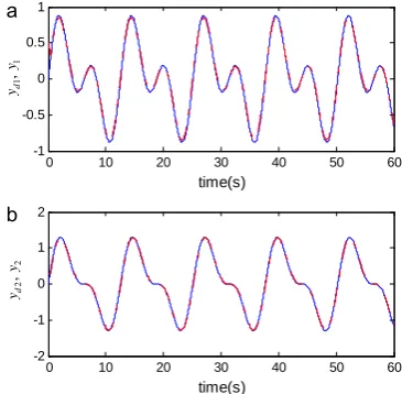
Figure 1. (a) The first reference signal yd1(solid line) and the subsystem output y1(dashed line); (b) The second reference signal
2 d
y (solid line) and the subsystem output y2(dashed line).
Simulation results are shown in Figs. 1-3. Fig. 1(a) and 1(b) present the response curves of system outputs
1, 2
y y and the reference signalsyd1, yd2. Fig.2 show that the
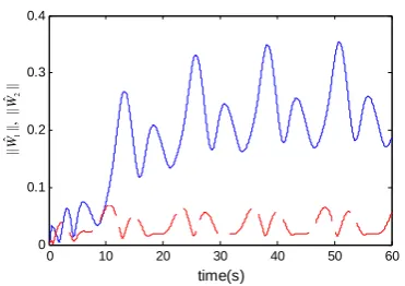
reasonable range. Fig. 3 illustrates the L2 norms of the
NNs weights adaptation. Comparing with the results [16], the results illustrate the control performance of the proposed scheme.
0 10 20 30 40 50 60
-4 -2 0 2 4
time(s)
0 10 20 30 40 50 60
-2 -1 0 1 2
time(s)
1
u
2
u
Figure 2. (a) The control u1of the first subsystem; (b) the control 2
u of the second subsystem.
0 10 20 30 40 50 60
0 0.1 0.2 0.3 0.4
time(s)
12
ˆˆ
||
||,
||
||
WW
Figure 3. L2 norms of the NNs weights adaptation: ||Wˆ1||(solid line) and ||Wˆ2||(dashed line).
V. CONCLUSION
In this note, the tracking control problem of uncertain nonlinear MIMO system with unknown time delays is addressed. A novel concise adaptive neural control scheme is developed with the “MLN” technique, which obtain some advantages: a concise structure and ease to implementation in control engineering, due to its computational burden. Both the problems of “explosion of complexity” and the “curse of dimensionality” are circumvented from the root causes, which are ever-presented in the current literatures on approximation-based adaptive control.
ACKNOWLEDGMENT
This work was supported by the National Natural Science Foundation of China (Grant No. 50979009), the Major State Basic Research Development Program of China (973Program) (Grant No. 2009CB320805) and the
Fundamental Research Funds for the Central University (Grant No. 2012TD002).
REFERENCES
[1] Marios M. Polycarpou, “Stable Adaptive Neural Control Scheme for Nonlinear Systems”, IEEE Transactions on Automatic Control, vol. 41, no. 3, pp.447-450, 1996. [2] Marios M. Polycarpou, M. J. Mears, “Stable Adaptive
Tracking of Uncertain Systems using Nonlinearly Parameterized On-line Approximators”, International Journal of Control, vol. 70, no. 3, pp.363-384, 1998. [3] Wangqiang Niu, Jianxin Chu, Wei Gu, “Robust tension
control of the anchor chain of the ship windlass under sea wind”, Journal of Computers, vol. 5, no. 4, pp.631-637, 2010.
[4] S.S. Ge, Cong Wang, “Direct Adaptive NN Control of a Class of Nonlinear Systems”, IEEE Transactions on Neural Networks, vol. 13, no. 1, pp.214-221, 2002.
[5] S.S. Ge, F. Hong, T.H. Lee, “Adaptive Neural Network Control of Nonlinear Systems with Unknown Time Delays”, IEEE Transactions on Automatic Control, vol. 48, no. 11, pp.2004-2010, 2003.
[6] Dan Wang, Jie Huang, “Neural Network-based Adaptive Dynamic Surface Control for a Class of Uncertain Nonlinear Systems in Strict-Feedback Form”, IEEE Transactions on Neural Networks, vol. 16, no. 1, pp.195-202, 2005.
[7] Min Wang, Xiaoping Liu, Peng Shi, “Adaptive Neural Control of Pure-Feedback Nonlinear Time-Delays Systems via Dynamic Surface Technique”, IEEE Transactions on Systems, Man, and Cybernetics—Part B, vol. 41, no. 6, pp.1681-1691, 2011.
[8] Z. Hou, Madan M. Gupta, Peter N. Nikiforuk, Min Tan, “A Recurrent Neural Network for Hierarchical Control of Interconnected Dynamic Systems”, IEEE Transactions on Neural Networks, vol. 18, no. 2, pp.466-480, 2007.
[9] S.S. Ge, K.P. Tee, “Approximation-based control of nonlinear MIMO time-delays systems”, Automatica, vol. 43, pp.31-43, 2007.
[10]Y. Liu, S. Tong, T. Li, “Observer-based adaptive fuzzy tracking control for a class of uncertain nonlinear MIMO systems”, Fuzzy Sets and Systems, vol. 164, no. 1, pp.25-44, 2011.
[11]Tie-Shan Li, Dan Wang, Gang Feng, Shao-Cheng Tong, “A DSC Approach to Robust Adaptive NN Tracking Control for Strict Feedback Nonlinear Systems”, IEEE Transactions on Systems, Man, and Cybernetics—Part B, vol. 40, no. 3, pp.915-926, 2010.
[12]M. Krstic, I. Kanellakopoulos, and P. Kokotovic, Nonlinear and Adaptive Control Design, New York: Wiley, 1995.
[13]D. Swaroop, J. Hedrick, P. Yip, J. Gerdes, “Dynamic surface control for a class of nonlinear systems”, IEEE Transactions on Automatic Control, vol. 45, no. 10, pp.1893-1900, 2000.
[14]Y. Yang, C. Zhou, “Robust adaptive fuzzy tracking control for a class of perturbed strict-feedback nonlinear systems via small-gain approach”, Information Sciences, vol. 170, pp.211-234, 2005.
[15]Y. Yang, X. Wang, “Adaptive NN tracking control of a class of uncertain nonlinear systems using radial-basis-function neural networks”, Neurocomputing, vol. 70, pp.932-941, 2007.
[17]Tieshan Li, Ronghui Li, Dan Wang, “Adaptive neural control of nonlinear MIMO systems with unknown time delays”, Neurocomputing, vol. 78, pp.83-88, 2012.
[18]Tieshan Li, ShaoCheng Tong, Gang Feng, “A Novel Robust Adaptive Fuzzy Tracking Control for a Class of Nonliear Multi-Input/Multi-Output Systems”, IEEE Transactions on Fuzzy Systems, vol. 18, no. 1, pp.150-160, 2010.
[19]Cong Wang, David J. Hill, S.S. Ge, Guanrong Chen, “An ISS-modular approach for adaptive neural control of pure-feedback systems”, Automatica, vol. 42, pp.723-731, 2006. [20]Hui Hu, Peng Guo, “Neural network adaptive control for a
class of matched SISO nonlinear uncertain systems with zero dynamics”, Journal of Computers, vol. 7, no. 6, pp.1490-1496, 2012.
Guoqing Zhang was born in 1987. He is a doctor degree candidate of Dalian Maritime University (DMU), China. His recent research areas are adaptive nonlinear control and its applications to marine control.
Xianku Zhang was born in 1968. He received his PH.D in 1998 from Dalian Maritime University(DMU), China, now he is a professor/doctor director of DMU. He is a scholarship leader of national key discipline named traffic information engineering and control and vice institute director of marine simulation and control. He authored or co-authored 120 papers, in which there are 50 papers indexed by SCI and EI, 9 books in the fields of ship motion control, robust control, intelligent control and computer programming. He has got 1 second class scientific awards from China and 2 second class scientific awards from Liaoning Province. His recent research areas are robust control, intelligent control and its applications to marine control. He is now responsible for a National Natural Science Foundation of China and Science Foundation of Ministry of Education of China, take part in a grant from the Major State Basic Research Development Program of China (973 Program).