Evaluation of Moving Average Model and Autoregressive Moving Average Model (ARMA) for Prediction of Industrial Electricity Consumption in Nigeria

(1)

http://www.sciencepublishinggroup.com/j/ajsea doi: 10.11648/j.ajsea.20170603.12

ISSN: 2327-2473 (Print); ISSN: 2327-249X (Online)

Evaluation of Moving Average Model and Autoregressive

Moving Average Model (ARMA) for Prediction of Industrial

Electricity Consumption in Nigeria

Idorenyin Markson

1

, Mfonobong Charles Uko

2

, Aneke Chikezie

2

1

Department of Mechanical Engineering, University of Uyo, Uyo, Nigeria

2_{Department of Electrical/Electronic and Computer Engineering, University of Uyo, Uyo, Nigeria}

Email address:

[email protected] (A. Chikezie)

To cite this article:

Idorenyin Markson, Mfonobong Charles Uko, Aneke Chikezie. Evaluation of Moving Average Model and Autoregressive Moving Average Model (ARMA) for Prediction of Industrial Electricity Consumption in Nigeria. American Journal of Software Engineering and Applications. Vol. 6, No. 3, 2017, pp. 67-73. doi: 10.11648/j.ajsea.20170603.12

Received: January 29, 2017; Accepted: March 30, 2017; Published: June 12, 2017

Abstract:

In this paper, evaluation of moving average model and autoregressive moving average model (ARMA) for prediction of industrial electricity consumption in Nigeria is presented. Industrial electricity consumption data obtained from Central Bank of Nigeria (CBN) Statistical Bulletin for the year 1979-2014 is used to determine the model parameters and prediction performance in terms of Root Mean Square Error (RMSE) and Coefficient of determination r2 values. The results show that the Autoregressive Moving Average (ARMA) model with coefficient of determination value of 66.0% and RMSE value of 68.628 gives better prediction performance than the Moving Average with coefficient of determination value of 42.6% and value of 84.749. However, coefficient of determination value of 66% is not particularly adequate for acceptable prediction accuracy. In that case, for better prediction accuracy for the industrial electricity consumption in Nigeria, other models may need to be examined apart from the two models considered in this paper.

Keywords:

Moving Average Model, Autoregressive Moving Average Model, Industrial Electricity Consumption, Prediction Accuracy, Time Series Models

1. Introduction

Globally, reliable and adequate electricity supply has been identified as paramount to socio-economic and technological development of every nation [1-8]. Particularly, the industrial sector with their job creation and poverty alleviation potentials is heavily reliant on electricity. In this wise, electricity is central to industrialization of any nation [9-13]. However, in Nigeria, there has been perennial acute shortage of power supply [14-16]. Some of the challenges include insufficient power generation, excessive power losses, poor maintenance of power plants, lack of political will to tackle the problems associated with the power sector.

In any case, since the last decades, Nigerian government has continued to introduce reforms in the power sector ranging from privation to expansion in the power generation and distribution capacities [17-25]. In all, there has been noticeable marginal improvement in the power supply across

the nation. However, the industrial sectors are still overwhelmed by grossly inadequate power supply. The effect has been on high cost of production in Nigeria and disproportional dependence on imported goods. In order to plan for adequate power supply to the industrial sector, the existing and projected industrial energy demand profile is needed. In this wise, models need to be developed and evaluated for prediction and possibly forecasting of the industrial electricity consumption in Nigeria.

(2)

performance is expressed in terms of Root Mean Square Error (RMSE) and Coefficient of determination .

2. Theoretical Background

In this paper, two time series models are considered, namely, Moving Average Model and Autoregressive Moving Average Model (ARMA). The two models are used to predict industrial electricity consumption in Nigeria. The prediction performance of the two models are then compared in terms of RMSE and r2 values.

2.1. Moving Average Model (MA) (of Order 1)

The moving average model of order 1 is given as;

0 1 1

t t t

Y = θ θ ε− ₋ +U (1)

0

θ and θ1 are the model parameters and Ut is the error

term with mean 0 and constant variance. Making Ut the subject in equation (1) gives

0 1 1

t t t

U = Y −θ θ ε− ₋ (2)

(

)

2 2

0 1 1

t t t

U = Y −θ +θ ε₋ (3)

Let 1 n t i S U =

=

∑

(4)

Taking partial derivatives of equation (3) with respect to

0

θ and θ1 gives

(

)

2

0 1 1

1

n

t t

t

S Y

θ θ ε

₋

=

∑

− + (5)

(

0 1 1

)

1 0 2( 1) n t t t S

Y θ θ ε

θ −

=

∂ ₌ ₋ ₋ ₊

∂

∑

(6)

0 1 1

1 2

2

n n

t t

Y n

θ θ

ε

−

= =

 

= − _ − + _



∑

 (7)

( )(

1 0 1 1

)

1 1

2

n

t t t

t S Y ε θ θ ε θ − − = ∂ _{= −} _ ₋ ₊ _  

∂

∑

(8)

2

1 0 1 1 1

2 2 2

2

n n n

t t t t

t t t

Y

ε

−

θ

ε

−

θ

ε

−

= = =

 

= − _ − + _



∑

 (9)

Setting

0 S θ ∂

∂ and 1

0

S θ ∂ ₌

∂ gives

0 1 1

1 2

0

n n

t t

Y n

θ θ

ε

₋

= =

− + =

∑

(10)

2

0 1 1

1 2 1

n n n

t t

t t i

n

θ

ε

₋ Y

= = =

− =

∑

(11)

2

1 0 1 1 1

2 2 2

0

n n n

t t t t

t t t

Y

ε

−

θ

ε

−

θ

ε

−

= = =

− + =

∑

(12)

2

0 1 1 1 1

1 1 2

n n n

t t t t

t t t

Y

θ

ε

−

θ

ε

−

ε

−

− − =

− =

∑

(13)

Arranging equations 10 to 13 in matrix form gives

1 2 2 1 1 2 2 n t t n n t t t t n ε ε ε − = − − = =   −       −    

∑

2 0 1 1 2 n t t n t t t Y Y θ θ _ε = − =      _{ } _ =   _ _      

∑

(14)

Let

M3 =

1 1 1 1 2 2 n n t t t t n n

t t t t

t t Y Y ε ε ε ε = = − − = =   −       −    

∑

(15)

3 p

= 0

1 θ θ      , 2 3 1 2 n t t n t t t Y V Y ε = − =       =      

∑

(16)

Then equation 14 becomes

3 3 3

p M =V (17)

1

3 3 3

p =M V− (18)

The solution of equation (18) gives the parameters of the Moving Average model.

2.2. Autoregressive Moving Average Model, (ARMA)

The ARMA can be expressed as:

0 1 1 1 1

t t t t

Y = β β+ Y₋ − θ ε₋ + a (19) Where, β β θ0, 1, 0andθ1are the parameters of the model

and a_tis the error term.

0 1 1 1 1

t t t t

a = Y −β − βY− +θ ε− (20)

(

)

2

0 1 1 1 1

t t t t

a = Y −β − βY− +θ ε− (21) Let D denote sum of square errors

Therefore; 2 1 n t t D a =

=

∑

(22)

(3)

(

0 1 1 1 1

)

1 0

2( 1)

n

t t t

t

D

Y β βY θ ε

β − −

=

∂ = − − − +

∂

∑

(23)

0 1 1 1 1

1 2 2

2

n n n

t t t

Y n

β

Y₋

θ

ε

₋

= = =

 

= − _ − − + _

 

∑

(24)

1 0 1 1 1 1

1 1

2( 1) ( ) ( )

n

t t t t

t

D

Y Y β βY θ ε

β − − −

=

∂ = − − − +

∂

∑

(25)

2

1 0 1 1 1 1 1 1

2 2 2 2

2

n n n n

t t t t t t

t t t t

Y Y₋ β Y₋ β Y₋ θ Y₋ε₋

= = = =

 

= − _

∑

−

∑

−

∑

+

∑

_ (26)

(

1

)(

0 1 1 1 1

)

1 1

2( 1)

n

t t t t

t D Y Y ε β β θ ε θ − − − = ∂ = − _ − − + _

∂

∑

(27)

2

1 0 1 1 1 1 1 1

2 1 2 2

2

n n n n

t t t t t t

t t t t

y y

ε− β ε− β ε− − θ ε −

= = = =

 

= −  − − + 



∑

 (28)

Setting 0 , D β ∂ ∂ then;

0 1 1 1 1

1 2 2

0

n n n

t t t

Y n

β

Y₋

θ

ε

₋

= = =

− − + =

∑

(29)

0 1 1 1 1

2 2 1

n n n

t t t

n

β

Y₋

θ

ε

₋ Y

= = =

⇒ ₋

∑

₊

∑

₌

∑

₍₃₀₎

Setting

1 D β ∂

∂ to zero

2

1 0 1 1 1 0 1 1 1 1

2 2 2 2 2

0

n n n n n

t t t t t t t

t t t t t

Y₋Y β Y₋ β Y₋ θ Y₋ θ Y₋ε₋

= = = = =

− − − + =

∑

(31)

2

0 1 1 1 1 1 1 1 1

2 2 2 2 2

n n n n n

t t t t t t t

t t t t t

Y Y Y Y Y Y

β ₋ β ₋ θ ₋ ₋ε₋ ₋

= = = = =

+ + − =

∑

(31)

Setting

1 D θ ∂

∂ to zero,

(

1

)(

0 1 1 1 1

)

1 1

2( 1)

n

t t t t

t D Y Y ε β β θ ε θ − − − = ∂ = − _ − − + _

∂

∑

(32)

2

1 0 1 1 1 1 1 1

2 2 2 2

2 0

n n n n

t t t t t t

t t t t

Y Y

ε− β ε− β ε− − θ ε −

= = = =

 

= −  − − + =



∑

 (33)

Divide through by -2 gives

2

0 1 1 1 1 1 1 1

2 2 2 2

n n n n

t t t t t t

t t t t

Y Y

β

ε

₋

β

ε

₋ ₋

θ

ε

₋

ε

₋

= = = =

+ − =

∑

(34)

Arranging the sets of equations 29 to-34 in matrix form give

1 1

2 2

2

1 2 1 1

2 2 2

2

1 1 1 1

2 2 2

n n t t t t

n n n

t t t t t t t

n n n t t t t t t t

n y

y y y

y ε ε ε ε ε − − = = − − − − = = = − − − − = = =         −          

∑

0 1 1 β β θ           = 1 1 2 1 2 n t t n t t t n t t t y y y y ε = − = − =                  

∑

(35) Let 1 1 2 2 2

4 1 2 1 1

2 2 2

2

1 1 1 1

2 2 2

n n t t t t n n n

t t t t t t t

n n n t t t t t t t

n y

M y y y

y ε ε ε ε ε − − = = − − − − = = = − − − − = = =         = −         

∑

, 0 4 1 1 p β β θ     =_ _     and 1 4 1 2 1 2 n t t n t t t n t t t y

V y y

y ε = − = − =         =         

∑

. Hence, equation 35 becomes:

4 4 4

M p

=

V

(36)

Making p₄ the subject of the formula in equation (36) gives

1 4

4 4

p

=

M

−

V

(37)

The solution of equation (37) gives the parameters of the ARMA model.

2.3. Performance Evaluation of the Models 2.3.1. Coefficient of Determination

The coefficient of determination is used to determine the effectiveness of using the models in predicting the predict industrial electricity consumption in Nigeria. gives the coefficient of the total variance in the department variable explained by the model.

2 RSS

r TSS

= (38)

RSS for model is = 11 1 1 1

t t

p V Y JY n

  −   

Generally, the RSS is:

1 1 1

i i i t t

SSR p V Y JY n

 

= − 

  , i = 1, 2, 3, 4 (39)

TSS for model

1 = Y_t1*Y_t 1 Y JY_t1 _t n

  − 

  (40)

(4)

(SSE) = SST- SSR (41)

2.3.2. Root Mean Square Error (RMSE)

The Means Square Error (MSE) is computed using the formula:

(

)

2

1

1 n _ˆ

t t

i

MSE Y Y

n =

=

∑

− (42)

The Root Means Square Error (RMSE) is given as

RMSE = √MSE (43)

Where, Yt is the actual industrial electricity consumption

and Yˆt is the predicted value from the model.

3 Results and Discussions

3.1. Moving Average Model

Table 1. Summary results of model estimation for industrial electricity consumption using moving average model.

Variables Coefficient Standard. Error r2

(%) RMSE

0

θ 293.7405 24.9958 42.60 84.749

1

θ 0.8911 0.123077

Table 1 gives results showing the model parameters and the model performance parameters namely r2 and RMSE for the moving average model. Based on the results, the Moving Average (MA) model of order 1 for predicting the industrial electricity consumption in Nigeria is given as:

Yt = 293.7405 + 0.8911 εt−1 (44)

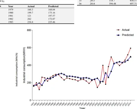
The results also show that the Moving Average model accounted for 42.6 percent of the variation in industrial electricity consumption (r2 = 0.426 = 42.6%). The actual and the Moving Average model predicted values of industrial electricity consumption are as shown in Table 1 and figure 1.

Table 2. Actual and predicted industrial electricity consumption using moving average industrial electricity consumption in Nigeria (MW/h).

S/N Year Actual Predicted

1 1979 160.3 191.35

2 1980 199.7 250.99

3 1981 121 244.00

4 1982 262 178.81

5 1983 254.4 350.47

6 1984 217.2 222.51

7 1985 259.8 279.7

8 1986 280.5 277.28

9 1987 294.1 297.43

10 1988 291.1 295.32

11 1989 257.9 294.14

12 1990 230.1 265.39

13 1991 253.7 260.92

14 1992 245.3 285.11

15 1993 237.4 260.54

16 1994 233.3 270.84

17 1995 218.7 259.92

18 1996 235.3 254.62

19 1997 236.8 273.15

20 1998 218.9 261.41

21 1999 191.8 253.75

22 2000 223.8 235.01

23 2001 241.9 276.75

24 2002 146.2 263.41

25 2003 196 187.55

26 2004 398 285.48

27 2005 182.3 396.34

28 2006 383.438 125.87

29 2007 494.01 496.05

30 2008 421.6 333.24

31 2009 428.954 383.66

32 2010 395.591 354.61

33 2011 426.37 345.39

34 2012 457.92 379.33

35 2013 518.7 383.48

36 2014 594.48 434.71

(5)

3.2. Autoregressive Moving Average (ARMA) Model

Table 3 gives results showing the model parameters and the model performance parameters namely r2 and RMSE for the autoregressive moving average (ARMA) model. Based on the results, the autoregressive moving average (ARMA) model for predicting the industrial electricity consumption in Nigeria is given as:

Yt = 24264.43 + 9996 Yt-1 - 0.5259εt−1 (45)

Table 3. Summary results of model estimation for industrial electricity consumption using autoregressive moving average (ARMA) model.

Model Parameter Coefficient r2_(%) _RMSE

0

β 24264.43 66.0 68.628

1

β 0.9996

1

θ -0.5259

The results also show that the ARMA model accounted for 66 percent of the variation in industrial electricity consumption (r2 = 0.66 = 66 %). The actual and the ARMA model predicted values of industrial electricity consumption are as shown in Table 4 and figure 2.

Table 4. Actual and predicted industrial electricity consumption using autoregressive moving average (ARMA) Industrial electricity consumption (MW/h).

1 1979 160.3 168.04

2 1980 199.7 175.16

3 1981 121 197.57

4 1982 262 172.07

5 1983 254.4 225.46

6 1984 217.2 249.93

7 1985 259.8 245.18

8 1986 280.5 262.86

9 1987 294.1 281.96

10 1988 291.1 298.45

11 1989 257.9 305.7

12 1990 230.1 293.78

13 1991 253.7 274.35

14 1992 245.3 275.31

15 1993 237.4 271.83

16 1994 233.3 266.26

17 1995 218.7 261.39

18 1996 235.3 251.92

19 1997 236.8 254.8

20 1998 218.9 257.02

21 1999 191.8 249.71

22 2000 223.8 233.03

23 2001 241.9 239.42

24 2002 146.2 251.35

25 2003 196 212.29

26 2004 398 215.34

27 2005 182.3 312.63

28 2006 383.438 261.62

29 2007 494.01 330.07

30 2008 421.6 418.44

31 2009 428.954 430.61

32 2010 395.591 440.5

33 2011 426.37 429.89

34 2012 457.92 438.89

35 2013 518.7 458.57

36 2014 594.48 497.71

(6)

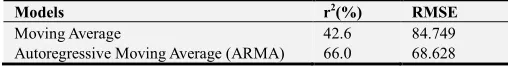
3.3. Evaluation of the Prediction Performance of the Models Table 5. Comparison of the Prediction Performance of the Moving Average Model and Autoregressive Moving Average Model (ARMA) Model.

Models r2_(%) _RMSE

Moving Average 42.6 84.749

Autoregressive Moving Average (ARMA) 66.0 68.628

Table 5 reveals that the Autoregressive Moving Average (ARMA) model with r2= 66.0% and RMSE = 68.628 gives better prediction performance than the Moving Average with r2=42.6% and RMSE = 84.749. As such, the ARMA model is recommended for forecasting industrial electricity consumption in Nigeria. However, r2 value of 66% is not particularly adequate for acceptable prediction accuracy. In that case, for better prediction accuracy, other models may need to be examined apart from the two models considered in this paper.

4. Conclusion

Moving Average Model and Autoregressive Moving Average Model (ARMA) are evaluated for their suitability in the prediction of the industrial electricity consumption in Nigeria. Industrial electricity consumption data from 1979-2014 is used to determine the model parameters and prediction performance in terms of RMSE and values. In all, ARMA model gives better prediction performance than the Moving Average model. However, the relatively low values for the two models shows that the models are not particularly adequate for prediction of the industrial electricity consumption in Nigeria. In that case, for better prediction accuracy, other models may need to be examined.

References

[1] Faridi, M. Z., & Murtaza, G. (2014). Disaggregate energy consumption, agricultural output and economic growth in Pakistan.

[2] Onakoya, A. B., Onakoya, A. O., Jimi-Salami, O. A., & Odedairo, B. O. (2013). Energy consumption and Nigerian economic growth: An empirical analysis. European Scientific Journal, 9(4).

[3] Sambo, A. S. (2008). Matching electricity supply with demand in Nigeria. International Association of Energy Economics, 4, 32-36.

[4] Essien, A. U., & Igweonu, E. I. (2014). Coal based generation: a solution to Nigeria electricity problem. Int Archive Appl Sci Technol, 5(1), 74-80.

[5] Sambo, A. S., Garba, B., Zarma, I. H., & Gaji, M. M. (2012). Electricity generation and the present challenges in the Nigerian power sector. Journal of Energy and Power Engineering, 6(7), 1050.

[6] Oluwalami, A. S. Review of Sustainable Energy and Electricity Generation from Non-Rewneable Energy Sources. Journal of Energy Technologies and Policy Vol.5, No.1, 2015

[7] Chukwu, P. U., Ibrahim, I. U., Ojosu, J. O., & Iortyer, H. A. (2014). Sustainable energy future for Nigeria: the role of engineers. Journal of Sustainable Development Studies, 6(2), 242.

[8] Oyedepo, S. O. (2012). Energy and sustainable development in Nigeria: the way forward. Energy, Sustainability and Society, 2(1), 15.

[9] Chong, C., Ni, W., Ma, L., Liu, P., & Li, Z. (2015). The use of energy in Malaysia: Tracing energy flows from primary source to end use. Energies, 8(4), 2828-2866.

[10] Barbiroli G. (2009 ) Principles of Sustainable Development - Volume II. Encyclopedia of Life Support Systems (EOLSS). Available at:

http://www.eolss.net/ebooklib/ebookcontents/e1-46a-themeco ntents.pdf Accessed on January 28th 2017.

[11] Seidler, R., & Bawa, K. S. (2016). Dimensions of sustainable development. RELIGION, CULTURE AND SUSTAINABLE DEVELOPMENT-Volume III, 161.

[12] Khatib, H. (2012). IEA world energy outlook 2011—A comment. Energy policy, 48, 737-743.

[13] Masjuki, H., Jahirul, M., Saidur, R., Rahim, N., Mekhilef, S., Ping, H., & Zamaluddin, M. (2006). Energy and electricity consumption analysis of malaysian industrial sector. Wood Wood Prod, 331(8).

[14] Kaunda, C. S., Kimambo, C. Z., & Nielsen, T. K. (2012). Potential of small-scale hydropower for electricity generation in Sub-Saharan Africa. ISRN Renewable Energy, 2012. [15] Uduma, K., & Arciszewski, T. (2010). Sustainable energy

development: the key to a stable Nigeria. Sustainability, 2(6), 1558-1570.

[16] Saifuddin, N., Bello, S., Fatihah, S., & Vigna, K. R. (2016). Improving Electricity Supply in Nigeria-Potential for Renewable Energy from Biomass. International Journal of Applied Engineering Research, 11(14), 8322-8339.

[17] Usman, Z. G., & Abbasoglu, S. (2014). An overview of power sector laws, policies and reforms in Nigeria. Asian Trans Eng, 4(2).

[18] Nnaji, B. A. R. T. (2011). Power sector outlook in Nigeria: government renewed priorities. presentation at Securities and Exchange Commission, Abuja, June.

[19] Okoro, O. I., & Chikuni, E. (2007). Power sector reforms in Nigeria: opportunities and challenges. Journal of Energy in Southern Africa, 18(3), 52-57.

[20] Wara, S. T., Abayomi-Alli, A., Umo, N. D., Oghogho, I., & Odikayor, C. (2009). An impact assessment of the Nigerian power sector reforms. In Advanced Materials Research (Vol. 62, pp. 147-152). Trans Tech Publications.

[21] Omoleke, I. I. (2011). Management of electricity generation and supply in Africa: The Nigerian experience. Journal of Public Administration and Policy Research, 3(10), 266. [22] Aminu, I., & Peterside, Z. B. (2014). The Impact of Privatization

of Power Sector in Nigeria: A Political Economy Approach. Mediterranean Journal of Social Sciences, 5(26), 111.

(7)

[24] Onyi-Ogelle, H. O. (2016). The implications of legal reform in the Nigeria power sector. African Research Review, 10(3), 279-289.

[25] Adenikinju, A. (2008). Efficiency of the Energy Sector and its Impact on the Competitiveness of the Nigerian Economy. International Association for Energy Economics, 27(32), 131-9.

[26] Almeshaiei, E., & Soltan, H. (2011). A methodology for electric power load forecasting. Alexandria Engineering Journal, 50(2), 137-144.

[27] Citroen, N., Ouassaid, M., & Maaroufi, M. (2015, March). Long term electricity demand forecasting using autoregressive integrated moving average model: Case study of Morocco. In Electrical and Information Technologies (ICEIT), 2015 International Conference on (pp. 59-64). IEEE.

[28] Meng, M., Shang, W., & Niu, D. (2014). Monthly electric energy consumption forecasting using Multiwindow Moving Average and Hybrid Growth models. Journal of Applied Mathematics, 2014.

[29] Meng, M., Niu, D., & Sun, W. (2011). Forecasting monthly

electric energy consumption using feature extraction. Energies, 4(10), 1495-1507.

[30] Karim, S. A. A., & Alwi, S. A. (2013). Electricity Load Forecasting in UTP Using Moving Averages and Exponential Smoothing Techniques. Applied Mathematical Sciences, 7(80), 4003-4014.

[31] As' ad, M. (2012). Finding the best ARIMA model to forecast daily peak electricity demand.

[32] Oyelami, B. O., & adedoyin Adewumi, A. (2014). Models for Forecasting the Demand and Supply of Electricity in Nigeria. American Journal of Modeling and Optimization, 2(1), 25-33. [33] Nowicka-Zagrajek, J., & Weron, R. (2002). Modeling

electricity loads in California: ARMA models with hyperbolic noise. Signal Processing, 82(12), 1903-1915.

[34] Central Bank of Nigeria (2006). CBN Statistical Bulletin Vol. 17 (December, 2006). Available at