Article Title & Authors

(1)

Performance Analysis of Public Banks in Turkey

Dr. Aşır Özbek

Vocational school, Kırıkkale University 71450 Kırıkkale, Turkey

Abstract

As financial institutions bridging investors and depositors, banks play an important role in the national economy. Efficient operation of the banking sector is crucial for the strategic objectives of banks as well as investors and the national economy. In other words, if the banking system does not work properly, national economy is badly affected. Therefore, performance measurement in the banking sector is an important issue that should be taken seriously.

In this study, the performance of public banks in Turkey, from 2005 to 2014, was measured by an integrated model combining the Analytic Hierarchy Process (AHP) and the Operational Competitiveness Rating method (OCRA). The input and output weights were calculated by AHP while efficiency of the banks was measured by OCRA. The study reveals that Vakifbank showed the highest performance until 2012, but Ziraat Bank took the lead in 2012.

Keywords:

Bank Performance, Analytic Hierarchy Process, Competitiveness Operational Rating, Turkey

JEL Classification: C6, C44, C67, G21

1.INTRODUCTION

Commercial banks are institutions that play a central role in the financial system of a country. Banking sector should keep working effectively, for this is vital for the national economy. It is because banks are financial agents that help use savings properly and undertake brokerage activities in a sector where resources are limited. Severe competition in the banking sector makes it essential for banks to use their deposits effectively. Therefore, they need to measure their efficiency at regular intervals and take necessary precautions to maximize their performance. Financial institutions with higher performance become more robust against financial crises caused by domestic or external influences. So they can evade a financial crisis with the least cost.

Measurement systems used in the performance and efficiency analysis in the banking sector can be divided into three basic groups structurally: ratio analyses, parametric and non-parametric methods. All the methods within these groups have their own advantages and disadvantages (İnan, 2000: 83). Parametric and non-parametric methods are called frontier analysis methods, which differ from each other depending on whether the technical or economic efficiency is measured (Ekren and Emirali, 2002: 8).

Measuring the efficiency and performance of banks involves a large number of inputs and outputs. However, there is no agreement on what these inputs and outputs are. Determined in the light of literature review, deposits, interest expenses and other expenses were used as the inputs in this study while loans, interest incomes and other incomes were used as the outputs. Obtained from the 2015 resources of the Union of Turkish Banks (www.tbb.org.tr), the data of 2005-2014 of 3 public banks in Turkey were used to present a model to measure the efficiency of the banks. It is an integrated model combining the Analytic Hierarchy Process (AHP) and the Competitiveness Operational Rating (OCRA). The input and output weights were determined by AHP while the efficiency of the three banks between 2005 and 2014 was measured by OCRA. The second part of the study focuses on the literature review. The third part deals with theoretical structure of AHP and OCRA methods. The application of the model was realized in the fourth part. In the final part, the results were analyzed and recommendations were made for future researchers.

2.LITERATURE REVIEW

(2)

and Eastern Europe between 2004-2008 by Andries (2011); the Chinese banks in 2007-2008 by Avkiran (2011); the banks of Nepal between 2007-2011 by Thagunn and Poudel (2012), and the efficiency of the Tunisian banks between 1990-2009 by Ayadi and Ellouze (2013). In addition, many other DEA based studies on the measurement and evaluation of bank performances can be found in the literature, such as Bauer et al. (1998), Camanho and Dyson (2006), and Portela and Thanassoulis (2007).

Different methods for measuring bank performances, separately or integrally used, can be found in the literature. For example, Mareschal and Brans (1991), Mareschal and Mertens (1992), Zopounidis and Doumpos (2010) used the PROMETHEE method. Home (2006) employed Gray Relation Analysis, Garcia et al. (2010) used goal programming, and Phuong Ta and Yin Har (2000) used the AHP.

There are also many studies based on the fuzzy approximation methods to measure financial parameters in the banking sector. For example, Weifeng and Huihuan (2008) as well as Ishizaka and Nguyen (2013) recommended the fuzzy AHP. Seçme et al. (2009), Mahrooz et al. (2013), Akkoç and Vatansever (2013) used the fuzzy AHP and fuzzy TOPSIS. Mandic et al. (2014) applied the fuzzy AHP and TOPSIS method to measure the performance of the banking sector in Serbia.

Among those who employed statistical methods are Ibrahim (2014) in the comparative study of Dubai Commercial Bank and Abu Dhabi National Bank; Abata (2014) in the performance measurement of the commercial banks in Nigeria; Kaya and Pastory (2013) in the performance analysis of 11 banks in Tanzania, and Kiptui (2014) in the performance measurement of the commercial banks in Kenya.

3.METHODOLOGY 3.1. Analytic Hierarchy Process

AHP is a Multiple Criteria Decision Making (MCDM) method developed by Saaty (1980), which is widely used to solve problems in different areas. AHP is an easy method whereby the decision alternatives, determined according to the factors set by the decision maker, are put in order of importance. AHP makes it possible to evaluate qualitative and quantitative criteria, and also it helps to add human judgments in the decision-making process. (Saaty, 1980)

The steps of the AHP process are described below (Saaty, 1994):

Step 1: Establishment of the Hierarchical Structure.

AHP defines the problem in a hierarchical structure consisting of minimum one factor in each level. It is based on the assumption that a factor below has an impact on another one above. Therefore, the aim is to determine by making pairwise comparisons to what extent a lower factor affects a higher one. AHP hierarchy should be established in at least three levels. The upper level includes the goal while the bottom one consists of the decision alternatives.

Step 2: Creating the Pairwise Comparison Matrices

While creating pairwise comparison matrices, factors in a level in the hierarchical structure are compared with the others in the upper level in pairs. The comparison of the alternatives is made separately to each factor, and as a result, there are as many pairwise comparison matrices as the number of factors. The comparison scale proposed by Saaty, shown in Table 1, is used in the creation of these matrices (Saaty, 2007). Such intermediate values as 2, 4, 6, and 8 can also be used if necessary.

The comparison of each element is realized in the corresponding level and the calibration of them is done on the numerical scale. This requires n(n-1)/2 comparisons, where n is the number of elements with the considerations that diagonal elements are equal or ‘1’ and the other elements will simply be the reciprocals of the earlier comparisons (Saaty, 1999). These comparison matrices are size n × n as formulated in Equation (1).

Table 1: Comparison Scale Intensity of

Importance Definition Explanation

1 Equal Importance Two activities contribute equally to the objective

3 Moderate importance Experience and judgment slightly favor one activity over another 5 Strong importance Experience and judgment strongly favor one activity over another

7 Very strong or demonstrated _importance An activity is favored very strongly over another; its dominance demonstrated in _practice

9 Extreme importance The evidence favoring one activity over another is of the highest possible order of _affirmation

A

1 a … a a 1 … a … … … …

… … … … … … … …

a a … 1

, a 1

(3)

Step 3: Creating the Normalized Decision Matrix.

The pairwise comparison matrix formulated in Equation (1) is normalized by using Equation (2)

a a

∑ a 2

Step 4: Calculating the Factor Weights

Factor weights are calculated by applying Equation (3) to the elements of the matrix normalized by Equation (2)

w 1

n a , i, j 1, 2, … , n 3

Step 5: Calculating Consistency Index and Consistency Ratio

The consistency of the matrix of the pairwise comparisons should be checked. If the Consistency Ratio (CR) is over 0.10, it means that the matrix is inconsistent. When this ratio is exceeded, the pairwise comparison matrix should be revised with different values (Saaty, 1980). To determine if the matrix is consistent, the Consistency Index (CI) coefficient must be calculated. CI is calculated by using Equation (5) (Saaty, 1994). In order to calculate CI, the , known as eigenvalue, should be calculated first. The eigenvalue is calculated by Equation (4). In addition, in order to evaluate the consistency, the Random Index (RI) value must be found. RI value corresponding to the size of each matrix is given in Table 2. After the CI and RI are determined, CR is calculated according to the Equation (6).

Table 2: Random Index Values

n 1 2 3 4 5 6 7 8 9 10 11 12 13 14

RI 0,00 0,00 0,58 0,90 1,12 1,24 1,32 1,41 1,45 1,49 1,51 1,53 1,56 1,57

λ 1

n.

∑ a . w

w 4

TI λ n

n 1 5

TO TI

RI 6

3.2. OCRA

OCRA is a simple and convenient method developed by Parkan (1994) to solve performance and efficiency analysis problems. OCRA is used in the measurement of the relative efficiency of the Product Units (PU) producing similar outputs using similar inputs. OCRA has been implemented in various areas successfully, such as investment banking, performance measurement of service buildings of public institutions, industrial enterprises, hotels and food production facilities (Peters and Zelewski, 2010).

In OCRA, input and output values should be different than zero to avoid zero division error in the normalization process. There is no way in OCRA to determine the input and output weights, called Calibration Constants in literature. The input and output weights can be calculated by simple scoring techniques such as cost-benefit analysis or by detailed evaluation methods such as AHP. It is possible to specify the input and output weights by using a scale in benefit-cost analysis. For example, in a scale going from 1 to 5; 5 shows the highest weight while1 symbolizes the lowest weight.

The sum of and values denoting the input and output weights should be 1 (Parkan, 2003). This is shown in Equation (7). The sum of the input and output weights may not be 1 depending on the method used. In this case, the normalized weight values are calculated by dividing the weight value of each factor, which is not normalized, by the total factor weight value.

a b 1 7

OCRA is a six-step process (Parkan and Wu, 2000; Peters and Zelewski, 2010):

Step 1: Calculation of the Unscaled Input Index

By taking the inputs into account, the unscaled Input Index, , is calculated for each PU by using the Equation (8).

i a max,…, X X min

,…, X

(4)

Step 2: Calculation of the Unscaled Output Index

Taking into account the outputs, unscaled output index, , is calculated for each PU, using the Equation (9).

o b Y min,…, Y min

,…, Y

, ∀n 1, … , K; Y 0; ∀k 1, … , K 9

Step 3: Scaling Input Indices

The scaling is done by subtracting the minimum value of the input index set from kth input index value of each PU by using the Equation (10).

I i min

,…, i , ∀k 1, … , K 10

Step 4: Scaling Output Index

The scaling is done by subtracting the minimum value of the index set from kth output index value of each PU by using the Equation (11).

O o min

,…, o , ∀k 1, … , K 11

Step 5: Calculation of the Unscaled Efficiency Index

The unscaled efficiency index is calculated by adding the scaled input index value and output index value of each PU using the Equation (12).

e I O , ∀k 1, … , K 12

Step 6: Calculation of the Scaled Efficiency Index

The scaled efficiency index is calculated by subtracting the smallest element in the unscaled efficiency index from each of the elements in the set using the Equation (13).

E I O min

,…, I O , ∀k 1, … , K 13

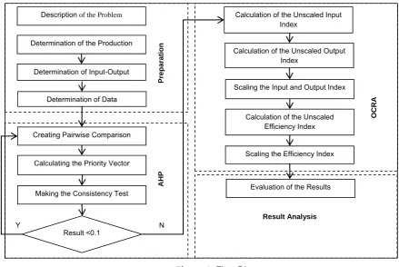
3.3. Flow Diagram of the Model

The data used to measure the efficiency of the public banks from 2005 to 2014 was obtained from the books of the relevant years, titled “Our Banks”, published by the Union of Turkish Banks (UTB) (Table 3). The literature review resulted in 2 inputs and 2 outputs: Deposits and interest expenses and other expenses as inputs and, loans and interest incomes and other incomes as outputs.

OCRA has no application for determining the input and output weights. The input and output weights were calculated by AHP. The performances of the banks for each year were determined by OCRA method. The flow chart of the model is shown in Figure 1 below.

Figure 1: Flow Diagram Description of the Problem

Determination of the Production U i

Determination of Input-Output

Determination of Data

Creating Pairwise Comparison

Calculating the Priority Vector

Making the Consistency Test

Calculation of the Unscaled Input Index

Calculation of the Unscaled Output Index

Result <0.1

Scaling the Input and Output Index

Calculation of the Unscaled Efficiency Index

Scaling the Efficiency Index

Evaluation of the Results

Y N

Preparatio

n

AHP

O

C

RA

(5)

4.RESULTS AND DISCUSSION

The data of all the three banks related to the years 2005-2014 was obtained from the books published by the Union of Turkish Banks (Table 3).

Table 3: Data of Banks

Name of Bank Ziraat Bank (ZB)

Year 2005 2006 2007 2008 2009 2010 2011 2012 2013 2014

PU (k) 1 2 3 4 5 6 7 8 9 10

Inputs Deposits 51.778 59.653 68.250 83.883 98.529 125.796 113.067 118.966 141.735 153.255

Interest expenses and other expenses 5.066 6.034 7.528 9.266 8.134 7.036 8.465 7.910 6.631 9.558

Outputs Loans 13.425 17.371 21.604 30.836 36.729 57.443 71.430 71.426 111.048 141.915

Interest incomes and other incomes 8.956 10.317 12.096 14.304 15.016 13.913 14.736 16.090 16.698 20.345

Name of Bank Halkbank (HB)

Year 2005 2006 2007 2008 2009 2010 2011 2012 2013 2014

PU (k) 11 12 13 14 15 16 17 18 19 20

Inputs Deposits 20.898 27.188 30.841 40.271 43.950 54.782 66.247 79.974 100.756 103.708

Outputs Loans 6.219 11.646 18.121 25.836 34.458 44.296 56.216 65.894 84.848 101.677

Name of Bank Vakifbank (VB)

Year 2005 2006 2007 2008 2009 2010 2011 2012 2013 2014

PU (k) 21 22 23 24 25 26 27 28 29 30

Inputs Deposits 22.946 24.842 28.863 37.120 44.652 47.701 60.939 67.242 81.533 91.757

Outputs Loans 11.905 18.043 23.470 30.502 34.573 44.861 57.309 68.133 86.752 104.584

The input and output weights were determined by means of AHP after the creation of pairwise comparison matrices. Then the matrix was normalized and subsequently, the factor weights, called the Priority Vector (PV), were calculated by means of the Equations (2) and (3). Table 4 shows the pairwise comparison matrix, and PV.

Table 4: Pairwise Comparison Matrix and Priority Vector

Deposits Interest expenses and

other expenses Loans

Interest incomes and other incomes PV

Deposits 1,000 7,000 1,000 7,000 0,451

Interest expenses and other

expenses 0,143 1,000 0,200 1,000 0,071

Loans 1,000 5,000 1,000 7,000 0,415

Interest incomes and other

incomes 0,143 1,000 0,143 1,000 0,065

After the input and output weights were determined, the unscaled input index was calculated. The unscaled input index, shown in table 5, was formed by the Equation (8). The input indices were calculated for all PUs.

Table 5: Unscaled Input Index

PU (k) 1 2 3 4 5 6 7 8 9 10

ZB 2,3303 2,1301 1,8979 1,5063 1,2255 0,6714 0,9014 0,7915 0,3400 0,0000

PU (k) 11 12 13 14 15 16 17 18 19 20

HB 3,0678 2,9194 2,8168 2,5911 2,5417 2,3250 2,0574 1,7390 1,2949 1,1698

PU (k) 21 22 23 24 25 26 27 28 29 30

VB 3,0398 2,982 2,868 2,666 2,538 2,4781 2,1782 2,0089 1,708 1,4158

(6)

Table 6: Unscaled Output Index

PU (k) 1 2 3 4 5 6 7 8 9 10

ZB 0,5609 0,8462 1,1575 1,8093 2,2141 3,5786 4,5254 4,5470 7,2010 9,3200

PU (k) 11 12 13 14 15 16 17 18 19 20

HB 0,0020 0,3823 0,8341 1,3666 1,9417 2,5976 3,4116 4,0837 5,3604 6,5184

PU (k) 21 22 23 24 25 26 27 28 29 30

VB 0,3266 0,7161 1,0650 1,5085 1,7418 2,3240 3,0755 3,7646 4,8618 5,9864

In the next step, the Equation (10) was used to do the scaling. Thus, the PU with the lowest value was given 0. The Scaled Input Index is shown in Table 7.

Similarly, the output index values of the PUs were also scaled. Table 8 shows the scaled output index.

After creating the scaled index for the inputs and outputs, the Unscaled Efficiency Index (UEI) was formed by using the Equation (12). Table 9 shows the UEI for the PUs.

Finally, by subtracting the smallest element in the UEI from each of the elements in the set using the Equation (13), the scaled efficiency index (SEI) was calculated. Table 10 gives the scaled efficiency index for the PUs.

Table 8: Scaled Output Index

PU (k) 1 2 3 4 5 6 7 8 9 10

ZB 0,5588 0,8442 1,1555 1,8073 2,2121 3,5766 4,5233 4,5450 7,1990 9,3179

PU (k) 11 12 13 14 15 16 17 18 19 20

HB 0,0000 0,3803 0,8321 1,3646 1,9397 2,5956 3,4095 4,0817 5,3583 6,5164

PU (k) 21 22 23 24 25 26 27 28 29 30

VB 0,3775 0,8039 1,1830 1,6703 1,9418 2,6244 3,4718 4,2248 5,4801 6,7158

Table 9: Unscaled Efficiency Index

KVB (k) 1 2 3 4 5 6 7 8 9 10

ZB 2,8892 2,9743 3,0534 3,3135 3,4376 4,2480 5,4248 5,3365 7,5390 9,3179

KVB (k) 11 12 13 14 15 16 17 18 19 20

HB 3,0678 3,2997 3,6489 3,9557 4,4814 4,9206 5,4670 5,8207 6,6532 7,6862

KVB (k) 21 22 23 24 25 26 27 28 29 30

VB 3,4173 3,7856 4,0513 4,3366 4,4802 5,1025 5,6500 6,2337 7,1881 8,1316

Table 10: Scaled Efficiency Index

KVB (k) 1 2 3 4 5 6 7 8 9 10

ZB 0,0000 0,0852 0,1642 0,4244 0,5485 1,3588 2,5356 2,4473 4,6499 6,4288

KVB (k) 11 12 13 14 15 16 17 18 19 20

HB 0,1786 0,4105 0,7597 1,0665 1,5922 2,0314 2,5778 2,9315 3,7640 4,7970

KVB (k) 21 22 23 24 25 26 27 28 29 30

VB 0,5281 0,8964 1,1621 1,4474 1,5911 2,2133 2,7608 3,3446 4,2989 5,2424

Table 7: Scaled Input Index

PU (k) 1 2 3 4 5 6 7 8 9 10

ZB 2,3303 2,1301 1,8979 1,5063 1,2255 0,6714 0,9014 0,7915 0,3400 0,0000

PU (k) 11 12 13 14 15 16 17 18 19 20

HB 3,0678 2,9194 2,8168 2,5911 2,5417 2,3250 2,0574 1,7390 1,2949 1,1698

PU (k) 21 22 23 24 25 26 27 28 29 30

(7)

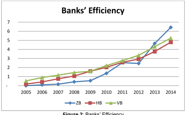
The AHP-OCRA based study with public banks demonstrated that VB had showed the best performance till 2012. It was found that starting from 2012, ZB started operating with higher efficiency (Figure 2).

Figure 2: Banks’ Efficiency

5.CONCLUSION AND RECOMMENDATIONS

The evaluation of the inputs-outputs using AHP showed that the Deposits was found to be the highest weight factor with 45.1%. The loans was the second most important factor after the deposits with 41.5%. The Interest and non-interest expenses, and Interest incomes and other incomes were found to be the least important inputs and outputs.

The AHP-OCRA based study showed that VB had the highest efficiency until 2012. Starting from 2013, ZB was found to be showing the best performance. Between 2005 and 2012, the 1st place in ranking was occupied by VB. HB was the 2nd, and ZB was the 3rd. In 2012, HB was the least efficient bank. The efficiency ranking as from 2013 showed that the 1st place was held by ZB, the 2nd by VB, and the 3rd by HB. The study also showed that starting from 2012, ZB increasingly showed a serious efficiency, and became the most efficient bank in 2013 although it was the most inefficient bank until 2012.

The model put into practice in this study based on AHP-ORCA can be compared with future studies based on other DEA models as well as such frequently used MCDM methods as MOORA (Multi-Objective Optimization on the basis of Ratio Analysis), VIKOR (Vise Kriterijumska Optimizacija I Kompromisno Resenje), and the Gray Correlation Analysis. Also, by changing the inputs and outputs, the results can be reanalyzed.

The model can run on software such as Excel, without requiring any compelling knowledge of mathematics. Thus, it could easily be implemented by sector managers. The model can also be used in many other areas by changing the inputs and outputs.

REFERENCES

Akkoç, Soner and Vatansever, Kemal, (2013). “Fuzzy performance evaluation with AHP and TOPSIS methods: evidence for Turkish banking sector after the global financial crisis”. Eurasian J. Bus. Econ. Vol 6, Nr 11, p. 53–74.

Andries, Alin Marius, (2011). “The Determinants of Bank Efficiency and Productivity Growth in the Central and Eastern European Banking Systems”. Eastern European Economics, Vol 49, Nr 6, p. 38-59.

Atan, Murat, (2003). “Türkiye Bankacılık Sektöründe Veri Zarflama Analizi ile Bilançoya Dayalı Mali Etkinlik ve Verimlilik Analiz”. Ekonomik Yaklaşım, Cilt 14, Sayı 48, s: 71-86.

Avkiran, Necmi K., (2011). “Association of DEA Super-Efficiency Estimates with Financial Ratios: Investigating the Case for Chinese Banks”. Omega, Vol 39, Nr 3, p. 323-334.

Ayadi, Inès and Abderrazak Ellouze, (2013). “Market Structure and Performance of Tunisian Banks”. International Journal of Economics and Financial Issues, Vol 3, Nr 2, p, 345-354.

Bauer, Paul. W., Berger, A. N., Ferrier, Gary. D. and Humphrey, David. B., (1998). “Consistency conditions for regulatory analysis of financial institutions: A comparison of frontier efficiency methods”. Journal of Economic and Business, Vol 50, Nr 2, p. 85–114.

Berger, Allen N. and Humphrey, David B., (1997). “Efficiency of financial institutions: International survey and directions for future research”.European journal of operational research, Vol 98, Nr 2, p: 175-212.

Camanho, A.S. and Dyson, R.G., (2006). “Data envelopment analysis and Malmquist indices for measuring performance”.

Journal of Productivity Analysis, Vol 26, Nr 1, p. 35–49.

‐ 1 2 3 4 5 6 7

2005 2006 2007 2008 2009 2010 2011 2012 2013 2014

Banks’ Efficiency

(8)

Demir, Y. and Astarcıoğlu, M., (2007). “Determining bank performance via financial prediction: An application in ISE”, Suleyman Demirel University. Journal of Business Administration and Economics Faculty, Vol 12, Nr 1, p. 273– 292.

Denizer, Cevdet A., Dinç, Mustafa and Tarımcılar, Murat, (2000). “Measuring bank efficiency in the pre and post liberalization environment: Evidence from the Turkish banking system”. World Bank Policy Research Working Paper, p. 2476.

Doumpos, Michael and Constantin Zopounidis, (2010). “A multicriteria decision support system for bank rating”. Decision Support Systems, Vol 50, Nr 1, p. 55-63.

Ekren, Nazım and Emiral, Fatih, (2002). "Türk bankacılık Sistemindeki Etkinlik Analizi (Veri Zarflama Analizi Uygulaması)".

Active Bankacılık ve Finans Dergisi, Yıl 4, Sayı 24, s: 6-27.

Erdem, Cumhur and Erdem, Meziyet Sema, (2008). “Turkish banking efficiency and its relation to stock performance”.

Applied Economics Letters, Nr 15, p. 207–211.

Fethi, Meryem Duygun and Pasiouras, Fotios, (2010). “Assessing bank efficiency and performance with operational research and artificial intelligent techniques: a survey”. European Journal of Operational Research, Vol 204, Nr 2, p: 189–198.

García, Fernando, Francisco Guijarro and Ismael Moya., (2010). “Ranking Spanish savings banks: A multi criteria approach”. Mathematical and Computer Modelling Nr 52, p.1058–1065.

Günay, E. Nur Özkan and Tektaş, Arzu (2006). “Efficiency Analysis of The Turkish Banking Sector in Precrisis and Crisis Period: A DEA Approach”. Contemporary Economic Policy, Vol 24, Nr 3, p. 418-431.

Ho, Chien-Ta, (2006). “Measuring bank operations performance: an approach based on grey relation analysis”. Journal of the Operational Research Society, Nr 57, p. 337–349.

https://www.tbb.org.tr/tr/banka-ve-sektor-bilgileri/istatistiki-raporlar/59, (29.05.2015)

İnan, Emre Alpan, (2000). “Banka etkinliğinin ölçülmesi ve düşük enflasyon sürecinde bankacılıkta etkinlik”. Bankacılar Dergisi, Sayı 34, s. 82-97.

Ishizaka, Alessio and Nguyen, Nam Hoang, (2013). “Calibrated fuzzy AHP for current bank selection”. Expert Syst. Appl. Vol 40, Nr 9, p. 3775–3783. http://dx.doi.org/10.1016/j.eswa.2012.12.089.

Işık, Ihsan, Meleke, Doğan and Meleke, Uğur, (2003). “Post-entry performance of de novo banks in Turkey”. In 10th Annual conference of the ERF.

Kao, Chiang and Liu, Shiang-Tai (2004). “Predicting Bank Performance with Financial Forecasts: A Case of Taiwan Commercial Banks”. Journal of Banking & Finance, Vol 28, Nr 10, p. 2353-2368.

Koçyiğit, M. Murat, (2013). “Mevduat Bankalarının Etkinliği ve Hisse Senedi Getirileri Arasındaki İlişki”. Muhasebe ve Finansman Dergisi, Sayı 57, s. 73-87.

Mahrooz, Amile, Maedeh Sedaghat and Morteza Poorhossein,(2013). “Performance evaluation of banks using fuzzy AHP and TOPSIS, case study: state-owned banks, particularly private and private banks in Iran”. Caspain J. Appl. Sci. Res., Vol 2, Nr 3, p. 128.

Mandic, Ksenija, Delibasic, Boris, Knezevic, Snezane and Benkovic, Sladjane, (2014). “Analysis of the financial parameters of Serbian banks through the application of the fuzzy AHP and TOPSIS methods”. Economic Modelling, Nr 43, p.30-37.

Mareschal, Bertrand and Jean Pierre Brans “BANKADVISER: an industrial evaluation system”. European Journal of Operational Research, Vol 54, Nr 3, p. 318–324.

Mareschal, Bertrand and Mertens, (1992). “BANKS: a multicriteria decision support system for financial evaluation in the international banking sector”. Journal of Decision Systems, Vol 50, Nr 1, p 175–189.

Parkan, Celik and Wu, Ming-Lu, (2000). “Comparison of three modern multicriteria decision-making tools”. International Journal of Systems Science, Vol 31, Nr 4, p. 497-517.

Parkan, Celik,(1994). “Operational Competitiveness Ratings of Production Units”. Managerial and Decision Economics, Vol 15, Nr 3, p. 201-221.

Parkan, Celik,(2003). “Measuring the effect of a new point of sale system on the performance of drugstore operations”.

Computers & Operations Research, Vol 30, Nr 5, p. 729-744.

Pasiouras, Fotios, (2008). Estimating the Technical and Scale Efficiency of Greek Commercial Banks: The Impact of Credit Risk, Off-Balance Sheet Activities, and International Operations”. Research in International Business and Finance, Vol 22, Nr 3, p. 301-318.

Peters, Malte L. and Zelewski, Stephan, (2010). “Performance Measurement mit hilfe des Operational Competitiveness Ratings (OCRA)”. WiSt Wirtschaftswissenschaftliches Studium, Vol 39, Nr 5, p.224.

Phuong Ta, Huu and Yin Har, Kar, (2000).” A study of bank selection decisions in Singapore using the Analytical Hierarchy Process”. International Journal of Bank Marketing, Vol 18, Nr 4, p. 170-180. http://dx.doi.org/10.1108/02652320010349058.

Portela, Maria Conceiçao A. Silva and Emmanuel Thanassoulis., (2007). “Comparative efficiency analysis of Portuguese bank branches”. European Journal of Operational Research, Vol 177, Nr 2, p. 1275–1288.

Saaty, Thomas L., (1980). The Analytic Hierarchy Process. McGraw-Hill, New York.

Saaty, Thomas L., (1994). Fundamentals of Decision Making and Priority Theory With The Analytical Hierarchy Proces. RWS Publ. Pittsburg.

Saaty, Thomas L., (1999). The Analytic Hierarchy Process for Decision Making. Kobe, Japan.

Saaty, Thomas. L. (2007). “The analytic hierarchy and analytic network measurement processes: applications to decisions under risk”. European Journal of Pure and Applied Mathematics, Vol 1, Nr 1, p. 122-196.

(9)

Stavarek, Daniel, (2006). “Banking Efficiency in the Context of European Integration”. Eastern European Economics, Vol 44, Nr 4, p. 5-31.

Thagunna, Karan Singh - Shashank Poudel, (2012). “Measuring bank performance of Nepali banks: A Data envelopment analysis (DEA) perspective”. International Journal of Economics and Financial Issues, Vol 3, Nr 1, p. 54-65. Weifeng, Xie and Gong, Huihuan, (2008). “Using fuzzy analytic hierarchy process and balanced scorecard for commercial

bank performance assessment”. In Business and Information Management, IEEE, ISBIM'08, Vol 1, p. 432-435. Yeh, Quey-Jen, (1996). “The Application of Data Envelopment Analysis in Conjunction with Financial Ratios for Bank

Performance Evaluation”. The Journal of the Operational Research Society, Vol 47, Nr 8, p. 980-988.

Yıldırım, Canan, (2002). “Evolution of Banking Efficiency within an Unstable Macroeconomic Environment: The Case of Turkish Commercial Banks”. Applied Economics, Vol 34, Nr 18, p. 2289-2301.