http://adb.sagepub.com/
Adaptive Behavior
http://adb.sagepub.com/content/19/6/451 The online version of this article can be found at:
DOI: 10.1177/1059712311419680 2011 19: 451
Adaptive Behavior
Oscar Javier Romero López
An evolutionary behavioral model for decision making
Published by:
http://www.sagepublications.com
On behalf of:
International Society of Adaptive Behavior
can be found at: Adaptive Behavior
Additional services and information for
http://adb.sagepub.com/cgi/alerts
Email Alerts:
http://adb.sagepub.com/subscriptions
Subscriptions:
http://www.sagepub.com/journalsReprints.nav
Reprints:
http://www.sagepub.com/journalsPermissions.nav
Permissions:
http://adb.sagepub.com/content/19/6/451.refs.html
Citations:
What is This?
- Nov 29, 2011 Version of Record
Adaptive Behavior 19(6) 451–475 ÓThe Author(s) 2011 Reprints and permissions:
sagepub.co.uk/journalsPermissions.nav DOI: 10.1177/1059712311419680 adb.sagepub.com
An evolutionary behavioral model for
decision making
Oscar Javier Romero Lo
´ pez
Abstract
For autonomous agents the problem of deciding what to do next becomes increasingly complex when acting in unpre-dictable and dynamic environments while pursuing multiple and possibly conflicting goals. One of the most relevant behavior-based models that tries to deal with this problem is thebehavior networkmodel proposed by Maes. This model proposes a set of behaviors as purposive perception–action units that are linked in a nonhierarchical network, and whose behavior selection process is orchestrated by spreading activation dynamics. In spite of being an adaptive model (in the sense of self-regulating its own behavior selection process), and despite the fact that several extensions have been proposed in order to improve the original model adaptability, there is not yet a robust model that can self-modify adap-tively both the topological structure and the functional purpose of the network as a result of the interaction between the agent and its environment. Thus, this work proposes an innovative hybrid model driven by gene expression program-ming, which makes two main contributions: (1) given an initial set of meaningless and unconnected units, the evolution-ary mechanism is able to build well-defined and robust behavior networks that are adapted and specialized to concrete internal agent’s needs and goals; and (2) the same evolutionary mechanism is able to assemble quite complex structures such as deliberative plans (which operate in the long-term) and problem-solving strategies. As a result, several properties of self-organization and adaptability emerged when the proposed model was tested in a robotic environment using a multi-agent platform.
Keywords
Intelligent and autonomous agents, evolutionary computation, gene expression programming, behavior networks, adap-tive behavior, automated planning
1 Introduction
An autonomous agent is a self-contained program that is able to control its own decision-making process, sen-sing and acting autonomously in its environment, and by doing so realize a set of goals or tasks for which it is designed. Usually these goals and tasks change dynami-cally through time as a consequence of internal and external (environmental) perturbations and, ideally, the agent should adapt its own behavior to these perturba-tions. Maes (1989, 1990, 1992) proposed a model for building such an autonomous agent that includes a mechanism for action selection (MASM) in dynamic and unpredictable domains, based on so-called beha-vior networks. This model specifies how the overall problem can be decomposed into subproblems, that is, how the construction of the agent can be decomposed into the construction of a set of component modules (behaviors) and how these modules should be made to interact. The total set of modules and their interactions provide an answer to the question of how the sensor data and the current internal state of the agent
determine the actions (effector outputs) and future internal state of the agent through an activation spreading mechanism that determines the best behavior to be activated in each situation. In addition, this model combines characteristics of both traditional planners and reactive systems: it produces fast and robust activity in a tight interaction loop with the envi-ronment, while at the same time allowing for some pre-diction and planning to take place.
Although original Maes networks do work in con-tinuous domains, they do not exploit the additional information provided by continuous states. Similarly, though there are mechanisms to distinguish different types of goals in MASM, there are no means to sup-port goals with a continuous truth state (such as ‘‘have
Fundacio´n Universitaria Konrad Lorenz, Bogota´, Colombia
Corresponding author:
Oscar J Romero Lo´pez, Fundacio´n Universitaria Konrad Lorenz, Carrera 9 Bis No. 62 - 43, Bogota´, Colombia
stamina’’) to become increasingly demanding the less they are satisfied. In regard to this, some extensions to the original behavior network model have been pro-posed (Dorer, 1999, 2004).
One of the most relevant weakness of the original Maes model is that the whole network model is fixed. It therefore requires both the network structure (e.g., spreading activation links) and global parameters of the network that define the characteristics of a particular application (e.g., goal-orientedness vs. situation-orient-edness, etc.) to be pre-programmed, and hence the agent has no complete autonomy over its own decision-making process. In order to resolve this problem, Maes (1991) proposed two mechanisms depending on real-world observations: a learning mechanism for adding/ deleting links in the network, and an introspection mechanism for tuning global parameters. The main problem with the former is that it does not use a real machine learning algorithm, but rather a simple statisti-cal process based on observations, so many hand-coded instructions are still required. With respect to the latter, it proposes a meta-network (another behavior network) that controls the global parameter variation of the first network through time, but the problem still remains: who is in charge of dynamically adapting the global parameters of the meta-network? It seems to be similar to the well-known homunculus problem of cognitive psychology; or, in colloquial terms, the Russian nested dolls (matryoska dolls) effect.
This work proposes a novel model based on gene expression programming (GEP; Ferreira, 2001) that, on the one hand, allows the agent to self-configure both the topological structure and the functional characteri-zation of each behavior network without losing the required expressiveness level; and, on the other hand, allows the agent to build more complex decision-making structures (e.g., deliberative plans and problem solving strategies) from the assembly of different kinds of evolved behavior networks. In contrast to the
beha-vior network extensions mentioned above, this
approach confers a high level of adaptability and flexi-bility, always producing, as a consequence, syntacti-cally and semantisyntacti-cally valid behavior networks.
The remainder of this article is organized as fol-lows. Section 2 outlines the operation of the behavior network model. Section 3 explains in detail how the behavior network model is extended using GEP. Section 4 illustrates the plan-extracting process using GEP. Section 5 outlines and discusses the results of the experiments. The concluding remarks are given in Section 6.
2 Behavior networks model
In the following, we describe the behavior network formalism. Since we do not need the full details for our
purposes, the description will be sketchy and informal at some points.
A behavior network (BN) is a mechanism proposed by Maes (1989) as a collection of competence modules that work in a continuous domain. Action selection is
modeled as an emergent property of an activation =
inhibition dynamics among these modules. A behavior
ican be described by a tuple hci,ai,di,aii.ciis a list of preconditions which have to be fulfilled before the behavior can become active ande=t(ci,s)is the execut-ability of the behavior in situationswheret(ci,s)is the (fuzzy) truth value of the precondition in situations.ai
and di represent the expected (positive and negative) effects of the behavior’s action in terms of an add list
and adelete list. Additionally, each behavior has a level of activation ai. If the proposition X about
environ-ment is true and X is in the precondition list of the behaviorA, there is an active link from stateX to action
A. If goalY has an activation greater than zero andY is in the add list of behaviorA, there is an active link from goalY to actionA.
Internal links include predecessor links, successor links, and conflicter links. There is a successor link from behavior A to behaviorB (A hasB as successor) for every propositionpthat is a member of the add list ofAand also a member of the precondition list ofB(so more than one successor link between two competence modules may exist). A predecessor link from moduleB
to module A (B has A as predecessor) exists for every successor link from A to B. There is a conflicter link from module A to module B (B conflicts with A) for every proposition pthat is a member of the delete list of B and a member of the precondition list of A. The following is the procedure to select an action to be exe-cuted at each step:
1. Calculate the excitation coming in from the envi-ronment and the goals.
2. Spread excitation along the predecessor, succes-sor, and conflicter links, and normalize the beha-vior activations so that the average activation becomes equal to the constantp.
3. Check any executable behaviors, choose the one with the highest activation, execute it, and finish. A behavior is executable if all the preconditions are true and if its activation is greater than the global threshold. If no behavior is executable, reduce the global threshold and repeat the cycle.
Additionally, the model defines five global para-meters that can be used to ‘‘tune’’ the spreading activa-tion dynamics of the BN and thereby affect the operation of the behavior network:
1. p: the mean level of activation.
selected. It is reset to its initial value when a mod-ule could be selected.
3. f: the amount of activation energy a proposition that is observed to be true injects into the network. 4. g: the amount of activation energy a goal injects
into the network.
5. d: the amount of activation energy a protected goal takes away from the network.
In the following section, we describe how the BN topology can be evolved in order to adapt to continu-ously changing goals and states of the environment. An approach to how complex decision-making structures (e.g., deliberative plans) can emerge from the interac-tion of multiple evolved BNs, is also presented.
3 Evolutionary behavior networks
We propose an extended version of Maes’ model, described above, that incorporates more sophisticated, rational, and complex processing modules than the sim-ple state machines proposed by Maes.1 In addition, it incorporates an evolutionary mechanism addressed by gene expression programming (GEP; Ferreira, 2001) in charge of evolving the BN topology, namely, the acti-vation=inhibition links among behaviors, the precon-ditions of each behavior, and the algorithm’s global parameters. This section explains how the chromo-somes of GEP can be modified so that a complete BN—including the architecture, the activation/inhibi-tion links, and the global parameters—can be totally encoded by a linear chromosome, even though it may be expressed as a nonlinear structure such as an expres-sion tree. It is also shown how this chromosomal orga-nization allows the adaptation of the network using the evolutionary mechanisms of selection and modifica-tion, thus providing an approach to the automatic design of BNs.
The main reason we have used GEP, instead of typi-cal genetic programming (GP) or other kinds of evolu-tionary algorithms (e.g., genetic algorithms, GA), as a behavior–network evolutionary mechanism is due to its powerful and robust capability of always creating com-plex and meaningful structures. The fundamental dif-ference between the three algorithms resides in the nature of the individuals: in GA the individuals are symbolic strings of fixed length (chromosomes); in GP the individuals are nonlinear entities of different sizes and shapes (parse trees); and in GEP the individuals are encoded as symbolic strings of fixed length (chro-mosomes), which are then expressed as nonlinear enti-ties of different sizes and shapes (expression trees). Thus, the structural and functional organization of GEP genes always guarantees the production of valid solutions, no matter how much or how profoundly the chromosomes are modified.
3.1 Genetic encoding of behavior networks
The network architecture is encoded in the familiar structure of a head and tail (Poli, Langdon, & McPhee, 2008). The head contains specialfunctionsthat activate the units, andterminals that represent the input units. The tail contains onlyterminals. Let us now analyze an example of how the BN is encoded into a GEP chromosome.
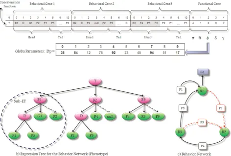
In Figure 1a, a linear multigenic chromosome is ini-tially generated in a random way and then modified by genetic operators. Each multigenic chromosome defines several behavioral genes and just one functional gene. Each behavioral gene encodes a different behavior’s structure, whereas the functional gene encodes the glo-bal parameters of the BN. We propose a multigenic chromosomal structure, which is more appropriate for evolving good solutions to complex problems because it permits the modular construction of complex, hier-archical structures, where each gene encodes a smaller and simpler building block (a behavior). These building blocks are physically separated from one another and thus can evolve independently. Not surprisingly, these multigenic systems are much more efficient than uni-genic ones (Ferreira, 2000). The details of the encoding process will be explained later.
The multigenic chromosome can then be translated into the whole expression tree shown in Figure 1b through the conversion process described by Poli et al. (2008) and Ferreira (2006). Here, it is possible to iden-tify three kinds of functions:B,D, andT. TheB func-tion is used for representing each behavior of the net, and it has an arity of three: the first branch is a set of preconditions, the second is a set of activation links that connects to other behaviors, and the third is a set of inhibition links that connects to other behaviors (dashed arrows). For example, behaviorB3 is activated when behavior B2 makes true precondition P4. After that, it spreads activation energy to behavior B1 through preconditionP5, and spreads inhibitory energy to behaviorB2 through preconditionP3. The DandT functions are connectivity functions that join two or three elements, respectively, of the same nature (e.g., behaviors, preconditions, goals, etc.). Note that the expression tree is composed of several subexpression trees (sub-ETs), each one representing the structure of a unique behavior in the net; hence each sub-ET has a particular organization that is encoded into one sepa-rate behavioral gene, and the whole expression tree (ET) models the entire behavior network.
Figure 1c depicts a basic BN with three behaviors (B1,B2, andB3), where the solid arrows denote excita-tory activation connections and the dashed arrows denote inhibition connections between behaviors. P1,
implementation the preconditions set for each behavior might be composed of a subset of sensory inputs (inter-nal and exter(inter-nal), a subset of active working memory elements, a subset of current subgoals, and a subset of motivational states (drives, moods, and emotions). G1 is an agent’s global goal pursued by behaviorB1.
In the example in Figure 1a, for each behavioral gene, positions from 0 to 3 encode the head domain (so both functions and terminals are allowed), and posi-tions from 4 to 12 encode the tail domain (where only terminals are allowed). Because each behavior defines variable sets of preconditions, activation links, and inhibition links, the corresponding genetic encoding spans along regions of different sizes into the
beha-vioral gene. Those regions are called open reading
frames(ORF; Ferreira, 2001). In GEP, what changes is not the length of genes, but rather the length of the ORF. Indeed, the length of an ORF may be equal to or less than the length of the gene. The noncoding regions are the essence of GEP and evolvability, because they allow the modification of the genome using all kinds of genetic operators without any kind of restriction. In fact, genetic operators can work on both regions (ORF and noncoding regions), always producing syntactically correct behavior networks.
Each sub-ET can be generated straightforwardly from chromosomal representation as follows: first, the start of a gene corresponds to the root of the sub-ET, forming this node in the first line; second, depending on the number of arguments to each element (functions may have a different number of arguments, whereas terminals have an arity of zero), in the next line are placed as many nodes as there are arguments to the functions in the previous line; third, from left to right, the nodes are filled, in the same order, with the ele-ments of the gene; and fourth, the process is repeated until a line containing only terminals is formed.
Because the process is bidirectional, inversely each behavioral gene can be easily inferred from the corre-sponding sub-ET as follows: the behavior function (B) of the sub-ET is encoded, and the algorithm then makes a straightforward reading of the sub-ET from left to right and from top to bottom (exactly as one reads a page of text). For instance, the sub-ET for behaviorB1 is encoded as:B1-D-G1-P2-P1-P5, and this is the ORF of its corresponding behavioral gene (i.e., the shadowy region for this gene in Figure 1).
The functional gene encodes an additional domain calledDp, which represents the global parameters of the
BN. For the functional gene, position 0 encodesp(the
mean level of activation), position 1 encodes u (the threshold for becoming active), position 2 encodes f
(the amount of energy for preconditions), position 3 encodesd (the amount of energy for protected goals), and position 4 encodes g (the amount of energy for goals). The values of global parameters are kept in an array and are retrieved as necessary. The number repre-sented by each position in the parameters domain indi-cates the order in the arrayDp. For example, position 0 in the functional gene (p) encapsulates the index ‘‘4’’ which corresponds to the value 92 in theDp array (in bold), and so on. For simplicity, Figure 1 only shows an array of 10 elements for parameter domainDp, but in the implementation we use an array of 100 elements, where each position encodes one numeric value between 0 and 100. Genetic operators guarantee that global parameters are always generated inside the domain of theDparray.
3.2 Special genetic operators
The evolution of such complex entities composed of different domains and different alphabets requires a special set of genetic operators so that each domain remains intact. The operators of the basic gene expres-sion algorithm (Ferreira, 2001) are easily transposed to behavior-net encoding chromosomes, and all of them can be used provided the boundaries of each domain are maintained so that alphabets are not mixed up. Mutation was extended to all the domains so that every different gene (behavioral or functional) was modified following its respective domain constraints (e.g., not replacing terminal nodes by function nodes in the tail region, etc.). Insertion sequence (IS) and root insertion sequence (RIS) transposition were also implemented in behavioral genes and their action is obviously restricted to heads and tails. In the functional gene we define only an IS operator (because the RIS operator is not appli-cable here) that works within theDp domain, ensuring
the efficient circulation of global parameters in the pop-ulation. Another special operator, parameters’ muta-tion, was also defined in order to directly introduce variation in the functional gene (i.e., global parameters region), selecting random values from theDparray.
The extension of recombination and gene transposi-tion to GEP-nets is straightforward, as their actransposi-tions never result in mixed domains or alphabets. However, for them to work efficiently (i.e., allow an efficient learning and adaptation), we must be careful in deter-mining which behavior’s structure elements and=or glo-bal parameters go to which region after the splitting of the chromosomes, otherwise the system is incapable of evolving efficiently. In the case of gene recombination and gene transposition, keeping track of behavioral and functional genes is not a difficult task, and these operators work very well in GEP-nets. But in one-point and two-point recombination where chromosomes can
be split anywhere, it is impossible to keep track of the behavior’s structure elements and global parameters. In fact, if applied straightforwardly, these operators would produce such large evolutionary structures that they would be of little use in multigenic chromosomes (Ferreira, 2006). Therefore, for our multigenic system, a special intragenic two-point recombination was used so that the recombination was restricted to a particular gene (instead of interchanging genetic material with other kinds of genes in the chromosome).
In summary, in order to guarantee the generation of valid BNs, all genetic operators have to comply with the following constraints:
In the first position of behavioral genes, only aB
(behavior) node can be inserted.
For the head region in behavioral genes:
— Mutation only by connectivity functions (D
andT), and by terminals such as precondi-tions (Pn) and goals (Gn).
— Transposition (IS and RIS) and one-point
and two-point recombination operators must follow the same syntactic validations as the mutation operator.
For the tail region in behavioral genes:
— Terminals can only be mutated, transposed, and recombined using elements from the tail domain, such as preconditions (Pn) and goals (Gn). No syntactic validations are required.
For global parameters in the functional gene: — Terminals can only be mutated, transposed,
and recombined using numeric values from parameters domainDp, that is, numeric val-ues between 0 and 100. No additional syn-tactic validations are required.
Finally, for each behavioral gene, the length of the
head h is chosen depending on the problem domain
(e.g., for the experiments we used h=10). This para-meter allows at least the encoding of all behaviors set. On the other hand, the length of the tailt is a function of bothhand the number of arguments nof the func-tion with more arguments (also called maximum arity), and is evaluated by Equation 1:
t=h(n1) +1 ð1Þ
In our case,n=3because this is the maximum arity for functionsBandT. If we defineh=10, thent=20, so the maximum fixed length for each behavioral gene is 30, and for the functional gene it is 5 (the maximum num-ber of global parameters).
3.3 Fitness functions for BN chromosomes
lower probability of being replicated in the next genera-tion of the evolugenera-tionary process. For the fitness evalua-tion we have taken into account the theorems proposed by Nebel and Babovich-Lierler (2004) and, addition-ally, we have identified a set of necessary and sufficient conditions that make behavior networks goal conver-ging. Note that all reinforcement parameters used in the next fitness functions are self-generated by the sys-tem from changes observed in the agent’s internal states, so that they do not require a priori or manual adjustment made by a designer.
We first define two fitness functions: one evaluates how well defined the behavior-network structure is, and the other evaluates the efficiency and functionality of the behavior network. First, the fitness function for evaluating the behavior-network structure is
FFSi=Ai+Bi+Ci+Di+Ei+Fi, ð2Þ
where i is a chromosome encoding a specific BN, and each term is defined as follows.
Ai: Is there at least one behavior of the net accom-plishing a goal? such that
A= a1, if9beh 2ijabeh \ G(t) 6¼ ; a2, otherwise
ð3Þ
where beh is any behavior of the network, abeh is the add list ofbeh,G(t)is a set of global goals,a1is a posi-tive reinforcement (by default 100), anda2is a negative reinforcement (by default100).
Bi: Are all behaviors of the net well connected? such
that
B=ncpb1+nupb2, ð4Þ
where ncp is the number of behaviors correctly
con-nected to others through successor and predecessor links (self-inhibitory connections are incorrect), nup is
the number of unconnected behaviors (no propositions at eitheradd listordelete list),b1is a positive reinforce-ment (by default +10), and b2is a negative reinforce-ment (by default20).
Ci: Are there any deadlock loops defined by the BN? such that
C=
(npc1) + (nnpc2), if the BN
has associated a global goal
c3, otherwise
8 < :
ð5Þ
wherenpis the number of behaviors that define at least
one path connecting to the global goal,c1is a positive reinforcement (by default +20), nnp is the number of
behaviors without a path between them and the global goal, c2 is a negative reinforcement (by default 10),
and c3 is another negative reinforcement (by
default50).
Di: Are all propositions (preconditions, add list, and delete list) of each behavior unambiguous? (e.g., the precondition set is ambiguous if it has propositions p
andpat the same time) such that
D=X
k
i=0
(nnad1) + (nad2), ð6Þ
where k is the total number of behaviors (behavioral genes) of the BN, nna is the number of propositions that are not ambiguous,d1is a positive reinforcement (by default +10), na is the number of ambiguous proposi-tions, and d2 is a negative reinforcement (by default
20).
Ei: Are all add-list propositions non-conflicting?
(e.g., a proposition that appears both in the add list and in the delete list—for the same behavior—is a con-flicting proposition), such that
E=X
k
i=0
(nncae1) + (ncae2), ð7Þ
wherekis the total number of behaviors of the BN,nnca
is the number of non-conflicting add-list propositions,
e1 is a positive reinforcement (by default +10), nca is the number of conflicting add-list propositions, ande2
is a negative reinforcement (by default20).
Fi: Are all delete-list propositions non-conflicting?
(e.g., a proposition that appears both in the precondi-tions set and in the delete list—for the same behavior— is a conflicting proposition), such that:
F=X
k
i=0
(nncdf1) + (ncdf2), ð8Þ
where k is the total number of behaviors of the BN,
nncdis the number of non-conflicting delete-list
proposi-tions, f1is a positive reinforcement (by default +10),
ncd is the number of conflicting delete-list propositions, andf2is a negative reinforcement (by default20).
Second, the fitness function for evaluating network functionality is:
FFEi=Gi+Hi+Ii+Ji+Li+Mi+Ni, ð9Þ
where i is a chromosome encoding a specific BN, and each term is defined as follows.
Gi: This term determines ifg (the amount of energy for goals) is a well-defined parameter. Because the para-meterg must reflect the ‘‘goal-orientedness’’ feature of the BN,
G=
100g1, if(RfreqG.0^Rg.0)_
(RfreqG\0^Rg\0)
g2, otherwise
8 <
whereRfreqG is the absolute variation rate which deter-mines how often a goal is activated or reactivated by the internal agent’s motivational subsystem. Therefore
RfreqG=
freqGcurfreqGpri freqGcur
, ð11Þ
where freqGcur is a frequency indicating how many
goals are activated in the current state, andfreqGpriis a frequency indicating how many goals were activated in a prior state.Rgis the absolute variation rate for
para-meterg:
Rg=
gcurgpri
gcur , ð12Þ
wheregcur is the value for g in the current state, and
gpriis the value ofgin the prior state. Finally,g1is the
absolute difference among the variation rates:
g1=jRfreqG Rgj; andg2is a negative reinforcement
(by default 100). Intuitively, when the frequency of activated goals increases over time, the global para-metergshould increase proportionally too.
Hi: This term determines iff(the amount of energy
for preconditions) is a well-defined parameter. Because the parameterf must reflect the ‘‘situation relevance’’ and ‘‘adaptivity’’ features of the BN,
H=
100h1, if(RfreqC.0^Rf.0)_(RfreqC\0^Rf\0)
h2, otherwise
ð13Þ
whereh1is the absolute difference among the absolute variation rates;h1=jRfreqC Rfj.RfreqCis a variation
rate (between current and prior states) that determines how often the environmental perturbations are per-ceived by the agent.Rf denotes the absolute variation
rate for parameterfandh2is a negative reinforcement (by default 100). Note that the absolute variation rates are treated similarly as in the termG.
Ii: This term determines ifp (the mean level of
acti-vation) is a well-defined parameter. Because the para-meter p must reflect the ‘‘adaptivity’’ and ‘‘bias to ongoing plans’’ features of the BN,
I=
100i1, if(RfreqSG.0^Rp.0)_
(RfreqSG\0^Rp\0)
i2, otherwise
8 <
: ð14Þ
where i1 is the absolute difference among the
absolute variation rates; i1=jRfreqSG Rpj. RfreqSG
is a variation rate (between a current and prior states) that determines the activation frequency of the sub-goals set that are associated to a current global goal.
Rp denotes the absolute variation rate for parameter
p and i2 is a negative reinforcement (by default
100). Absolute variation rates are treated similarly
as in the term G. Intuitively, if the environment requires the agent to address its actuation to the achievement of a hierarchical set of goals, the BN must increase the value ofpthrough time; otherwise, if the environment is quite dynamic and an adaptive
behavior is required, the parameter p should
decrease.
Ji: This term determines ifd(the amount of energy
for protected goals) is a well-defined parameter. Because the parameter d must reflect the ‘‘avoiding goal conflicts’’ feature of the BN,
J= 100j1, if(Rauto.0^Rd\0)_(Rauto\0^Rd.0)
j2, otherwise
ð15Þ
wherej1is the absolute difference between the absolute variation rates;j1=jRauto Rdj.Rautois the absolute
variation rate for the number of self-referenced loops identified by the agent between current and prior states (e.g., when the system identifies a circular reference of behavior activation such as: a!b, b!c, c!a). Rd
denotes the absolute variation rate for parameterdand
j2 is a negative reinforcement (by default 100). Intuitively, if Rauto increases, then Rd should decrease
proportionally, and vice versa.
Li: This term determines ifu(the threshold for
becom-ing active) is a well-defined parameter. Because the para-meter u must reflect the ‘‘bias to ongoing plans,’’ ‘‘deliberation,’’ and ‘‘reactivity’’ features of the BN,
L=
100l1, if(RfreqCE.0^Ru\0)_(RfreqCE\0^Ru.0)
l2, otherwise
ð16Þ
wherel1is the absolute difference among the absolute variation rates;l1=jRfreqCE Ru j.RfreqCEis the
abso-lute variation rate for the number of changing environ-mental elements between current and prior states (e.g., novel objects coming into the perception field, or per-ceived objects that change physically, etc.).Ru denotes
the absolute variation rate for parameteruandl2is a negative reinforcement (by default100). Intuitively, if
RfreqCE increases (i.e., the environment is more
dynamic), then Ru should decrease proportionally
(making the BN more reactive); but ifRfreqCE decreases,
thenRushould increase in order to make the BN more
deliberative.
M=m1X
k
i=0
eev, ð17Þ
wherem1is a positive reinforcement (by default +100) andkis the number of propositions defined by the add-list of the activated behavior (abeh). eev is a function that determines if the expected effect is included in the current state (S(t)), in other words, it validates if the condition9p2S(t)jp \ abeh 6¼ ;is true.
Ni: This term validates the delete-list efficiency of each behavior. If the current state includes a percept that corresponds to any delete-list’s proposition of any behavior, the behavior will receive a negative reinforce-ment (remember that the delete list represents the unex-pected effects which should not be present during behavior execution).
N=n1X
k
i=0
een ð18Þ
wheren1is a negative reinforcement (by default200) and k is the number of propositions defined by the delete-list of the activated behavior (dbeh).eenis a func-tion that determines if the unexpected effect is not included in the current state (S(t)), in other words, it validates if the condition 9p2S(t)jp \ dbeh = ; is true.
Finally, the whole fitness for each BN is calculated as
FFTi=FFSi+FFEi ð19Þ
All the elements of the function exert different (and in some cases, opposing) evolutionary and selective pres-sures. On the one hand, we have defined a function ele-ment for each of the most typical structural problems identified in behavior networks (such as terminating and dead-end networks, monotone networks, nonconverging acyclic networks, ambiguous and conflicting links, etc.). On the other hand, we have defined a function element for each kind of functional characterization of the beha-vior network (such as goal orientedness vs. situation orientedness, bias towards ongoing plans vs. adaptivity, deliberation vs. reactivity, and sensitivity to goal con-flicts). So the whole fitness function tries to model a multi-objective problem where the most suitable solu-tion will probably be found at an intermediate point.
4 Plan extraction
Another main contribution that our evolutionary approach makes is the capability to extract plans as HTN-like structures (HTN, hierarchical task networks; Sacerdoti, 1977) as a result of the interaction among behavior networks. In HTN planning, high-level tasks are decomposed into simpler tasks until a sequence of
primitive actions solving the high-level tasks is
generated. If the decomposition is not possible (e.g., because of colliding restrictions), the planner back-tracks and creates a different decomposition. However, in our proposal we don’t use a backtracking mechan-ism to infer a plan (which may be very expensive com-putationally when the plan grows in size), but we propose a mechanism that discovers a plan as an incre-mental composition of elements, from low-order
build-ing blocks to high-order tasks: building blocks
(symbolic and subsymbolic rules) ! behaviors! beha-vior networks!plans.2Thus, the main contribution we make in comparison with classic planners and meth-odologies (such as HTN planning) is that our approach does not need a priori definition of axioms, premises, and operators to generate a complex hierarchical plan.
The hierarchical plan is encoded as a linear structure of subtasks, which is evolved by GEP. Thus, a new plan is built and executed as follows:
1. A new plan is generated randomly as a genetic lin-ear structure (this will be explained later).
2. The genetic structure is translated into an expres-sion tree as in Section 3.
3. The expression tree is translated into a HTN-like structure.
4. The HTN-like structure is translated into an ordered tasks sequence as a result of applying the tree-traversal process in postorder.
5. Each subtask of the sequence is executed by a corresponding BN. The activated BN starts the spreading activation dynamics and selects an executable behavior. Each behavior is activated and the corresponding action is executed. The process continues until the associated subgoal is achieved by the BN.
6. After the BN achieves the subgoal, the next sub-task is selected as indicated by the linear order of the sequence (plan), and the process restarts in the previous step. The plan execution finalizes when there are no more subtasks to execute.
determine which ADFs are called upon in which main program and how they interact with one another.
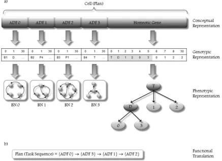
In Figure 2 we present a schematic representation of a plan as a cell structure that is formed by multiple ADFs and one homeotic gene. Each ADF corresponds to one BN with distinctive topology and functionality; in other words, every ADF is a multigenic chromosome that defines a set of behaviors and the spreading activa-tion dynamics between them in order to accomplish a subgoal through the continuous reorientation of the agent’s attention process. Thus, every ADF promises to achieve a subtask of the plan.
The homeotic gene builds a hierarchical structure as a HTN-like plan. Therefore, it defines how ADFs (goal-oriented behavior networks), which are function-ally independent from each other, interact through cooperative and competitive relationships with each other. In this way, the homeotic gene is able to control which BN is activated in every moment and which one is inhibited while the others cooperate in order to achieve a set of goals and subgoals. As shown in Figure 2, each BN (ADF) has a different topology, different set of goals, and different global parameters, and hence each hierarchical structure plan (cell) is distinctive from other plans (considering a multicellular system).
Homeotic genes have exactly the same kind of struc-ture as conventional genes and are built using an identi-cal process. They also contain a head and a tail domain. In this case, the heads contain linking functions (so called because they are used to link different ADFs) and a special class of terminals—genic terminals—rep-resenting conventional genes, which, in the cellular sys-tem, encode different ADFs; the tails contain only genic terminals.
It is worth pointing out that homeotic genes have their specific length and their specific set of functions and terminals. In our case, the homeotic gene uses the connectivity functions DandT (which were explained in Section 3.1) in order to link ADFs (terminals), and each terminal is a node that represents the index of the ADF in the corresponding cell. For instance, terminal ‘‘0’’ invokes ‘‘ADF 0,’’ terminal ‘‘1’’ invokes ‘‘ADF 1,’’ and so on. Figure 2a depicts a homeotic gene that encodes the following genetic sequence (just the ORF region):T-D-1-2-0-3. In Figure 2b, the plan is extracted as an ordered task sequence as a result of applying the tree-traversal process in postorder. Thus, the extracted plan indicates that initially ADF0 (BN0) is executed; when it finishes, ADF3 (BN3) is executed, then ADF1 (BN1), and finallyADF2(BN2).
It is important to note that the adaptive mechanism of these complex and hierarchical plans has an implicit co-evolutionary process: the evolutionary development of each separate decision-making structure (such as behaviors and BNs) affects the building of high-order cognitive structures such as plans. Co-evolution differs from ordinary unimodal evolutionary algorithms in terms of fitness function usage, because the evaluation process is based on interactions between individuals, in our case among BNs. Each BN represents a distinct component of the problem which has to collaborate with the others in order to construct an effective com-posite solution. In other words, the fitness function is nonstationary, but it is also based on the quality of co-existing individuals representing different problem components (De Jong & Pollack, 2004). Because the fit-ness measure is specified relative to other BN (as indi-viduals), the improvement of the quality of a partial population triggers further improvements in other populations. Intuitively, from Figure 2 it is also possi-ble to infer that each agent has a set of cells (each one modulating a hierarchical composite plan) which com-pete with each other for the right to solve a specific problem.
As a result, after a certain number of evolutionary generations, valid and better adapted cells are gener-ated inside the agent. A roulette-wheel method is used to choose the cells with the most likelihood of selection derived from their own fitnesses, and their components’ fitnesses (ADFs’ fitnesses). The cell’s fitness represents how good the interaction with the environment was during agent’s lifetime and is partially determined by feedback signals from the environment and the evalua-tion of a fitness funcevalua-tion.
4.1 Fitness function and feedback signal for plans
The evaluation of how good every generated plan is, is driven by two processes: (1) the internal simulationof every plan (cell); and (2) the later evaluation of the fit-ness functionfor every simulated plan.
For theinternal simulation process we use an antici-patory system that provides feedback about how opti-mal a plan would be if it were executed in the agent’s world. In other words, each plan (cell) is tested intern-ally through multiple simulated loops; at each step, an anticipatory system (driven by ananticipatory classifier system; Butz, Goldberg, & Stolzmann, 2002; Stolzmann, 1999) predicts the next state of the world that has the highest probability of occurring. In the anticipatory system, the structure of the stimulus– response rules (classifiers) is enhanced by an effect part representing an anticipation of the perceptive conse-quences of its action on an environment (the agent’s world). This effect part, associated with a learning pro-cess called the anticipatory learning propro-cess (ALP), enables the system to learn latently a complete internal
representation of the environment. The ALP represents the application of the anticipatory behavioral control into the system. Therefore, the anticipatory system combines the idea of learning by anticipation with that of the learning classifier systems framework (Booker, Goldberg, & Holland, 1989).
Thefitness functionused to evaluate the performance of each generated plan is based on a function of three terms:
FFPi=
ReinforcementiCosti Durationi
ð20Þ
whereFFPiis the fitness function for the simulated plan
i, and the other terms are described as follows.
Durationi: is the total period of time the simulated plan would take if it was executed by the agent in the world. This term is estimated as the sum of all pre-dicted time responses that the agent would take for every action.
Durationi= Xn
i=0
ALi, ð21Þ
wherenis the number of steps (concrete actions) neces-sary to achieve the target goal from the current state, and AL is the number of activation loops that the BN takes in every step to select an executable behavior (remember that spreading activation dynamics can exe-cute several loops before choosing an executable beha-vior). As you can see, the duration function (Di) is
inverse to the reinforcement function (Ri); so,
intui-tively, the fewer activation loops are necessary to achieve behavior activation, the stronger is the positive feedback signal.
Reinforcementi: is the estimated net amount of feed-back that the agent would collect if the plan was executed:
Reinforcementi= Xn
i=0
Rbeh,i+RBN,i, ð22Þ
whereRbeh,i is the estimated net reinforcement that the
current activated behavior (selected by the BN in every step i) receives after executing its action in the internal simulation.RBN,iis the estimated net reinforcement that
every BN receives after executing the simulated plan.
Rbeh,i is a prediction that the anticipatory classifier system makes about how much feedback (positive or negative) would be received by the behavior after executing its action. On the other hand, theRBN,i
rein-forcement corresponds to the evaluation of fitness function for every BN (as discussed for Equation 19).
Costi: is the estimated cost if the plan was executed,
Costi= Xn
i=0
Xr
j=0
Eni,j, ð23Þ
wherenis the number of simulated actions,ris the num-ber of resources (actuators) that the agent would use to carry out the actioni, andEni,jis the amount of energy
that would be required by the actuatorjat actioni. For example, if the agent is a robot that has to move boxes from one place to another, the costs required by the robot in every execution step would depend on the num-ber of actuators (e.g., an actuator to control the robot speed, an actuator to control the turn rate, an actuator to control a gripper, etc.) involved in every executed action, and on the amount of energy that would be needed to activate each one of these actuators. Note that the cost function is an optional term for the fitness func-tion and it has to be defined for each problem domain. Therefore, the way these two processes (internal simula-tion and fitness funcsimula-tion) interact with each other in order to validate a new plan is described as follows:
1. A set of plans (such as cells formed by ADFs) are generated using GEP operators.
2. For Each plan, do:
2.1. The agent perceives the current state. 2.2. While the plan simulation has not achieved
the final goal, do:
2.2.1. The corresponding BN (determined by the sequential order of the plan) is activated.
2.2.2. The winner behavior, which has
been selected by the spreading acti-vation dynamics of the activated BN, is executed.
2.2.3. The action that proposed the acti-vated behavior is executed into the (internal) simulated environment.
2.2.4. The statistics described above
(duration, cost, and reinforcement) are updated.
2.2.5. A new prediction of the next state is generated by the anticipatory system. 2.2.6. If it is possible to make a prediction of the world’s next state, the external sen-sory input is replaced by the prediction and the loop continues with step 2.2.1, otherwise, the simulation stops. 2.3. End While.
3. End For Each.
4. The overall fitness function for each plan (FFP
from Equation 20) is computed (taking into con-sideration all the feedback signals).
5. The plan with the highest fitness is selected:
bestPlan=maxj(FFP(j,i)) ð24Þ
6. The selected plan is executed by the agent.
5 Experimentation
In order to evaluate the proposed evolutionary decision-making model, the following aspects were considered:
1. Convergence rate of evolutionary structural design of BNs.
2. Comparison of convergence rates of evolutionary functional design of BNs using multiple experi-mental cases.
3. Convergence rate of evolutionary design of plans.
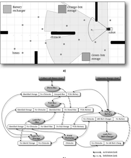
A simulated robotic environment was proposed to test the experiments. In the simulated environment, the robot had to collect different kinds of objects and then deliver them to specific storage boxes. The robot had to coordinate different kinds of tasks such as object search, object recognition, route planning, obstacle avoidance, battery recharging, object piling up, and so forth.
The simulated robotic environment was designed using the Player/Stage platform.3 Stage simulates a population of mobile robots moving within and sensing a two-dimensional bitmapped environment. Various sensor models are provided, including sonar, scanning laser rangefinder, pan-tilt-zoom camera with color blob detection, and odometry. In our simulation the robot (agent) was provided with four kinds of sensor inter-faces: sonar sensors, gps sensor, laser sensors, and fidu-cial sensors; and two kinds of actuator interfaces: position interface and gripper interface.
The sonar interface provides access to a collection of fixed range sensors, such as a sonar array. The gps interface provides access to an absolute position sys-tem, such as GPS. The laser interface provides access to a single-origin scanning range sensor, such as a SICK laser range-finder. The fiducial interface provides access to devices that detect coded fiducials (markers) placed in the environment. These markers work as reference points (fixed points) within the environment to which other objects can be related or which objects can be measured against. The fiducial sensor uses the laser sen-sor to detect the markers. The position interface is used to control a planar mobile robot base (i.e., it defines the translational and rotational velocities). The gripper interface provides access to a robotic gripper (i.e., it allows the robot to grasp and release objects). Figure 3 shows some of the robot interfaces used.
5.1 Convergence rate of evolutionary structural
design of BNs
of evolved BNs, we proposed a target BN that achieves two global goals of the agent: Collect-All-Boxes and Maintain-Energy. The main idea of this experiment is that the robot has to collect all the boxes, which are scattered everywhere in the world, and put them down at the corresponding storage, while also avoiding surrounding obstacles and rechar-ging the battery every time that it runs out of energy. The agent has to learn all the relationships between behaviors (activation and inhibition links) in the BN. Figure 4 depicts the world used in the experiment and
the target BN that the robot had to discover through the evolutionary process.
We proposed a population of 100 BNs. Each individ-ual BN was represented by a multigenic chromosome that was composed of seven behavioral genes (one for each behavior of the net), where each gene had a length of 30 elements (i.e., head length = 10 and tail length = 20), and one functional gene with a length of 5 ele-ments (one for each global parameter). Thus, the whole
chromosome has a length of 215 alleles (i.e., 30
7+5). The GEP parameters were defined both through
Figure 3. Robot interfaces.
Phenotype translation
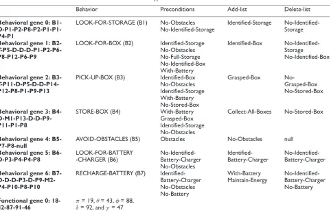
Behavior Preconditions Add-list Delete-list
Behavioral gene 0: B1- D-P1-P2-P8-P2-P1-P1-P4-P1
LOOK-FOR-STORAGE (B1) No-Obstacles No-Identified-Storage
Identified-Storage No-Identified-Storage
Behavioral gene 1: B2- T-P5-D-D-D-P1-P2-P6-P8-P12-P6-P9
LOOK-FOR-BOX (B2) Identified-Storage No-Obstacles No-Full-Storage No-Identified-Box With-Battery
Identified-Box No-Identified-Storage
No-Identified-Box
Behavioral gene 2: B3- T-P11-D-P5-D-D-P14-P12-P8-P1-P9-P13
PICK-UP-BOX (B3) Identified-Box No-Obstacles Identified-Storage With-Battery No-Stored-Box
Grasped-Box No-Grasped-Box No-Stored-Box
Behavioral gene 3: B4- D-M1-P13-D-D-P9-P11-P1-P8
STORE-BOX (B4) With-Battery Grasped-Box Identified-Storage No-Obstacles
Collect-All-Boxes No-Stored-Box
Behavioral gene 4: B5-P7-P8-null
AVOID-OBSTACLES (B5) Obstacles No-Obstacles null
Behavioral gene 5: B6-D-P3-P4-P4-P8
LOOK-FOR-BATTERY -CHARGER (B6)
No-Identified-Battery-Charger No-Obstacles
Identified-Battery-Charger
No-Identified-Battery-Charger
Behavioral gene 6: B7- D-D-D-P3-D-P9-M2-P4-P10-P8-P10
RECHARGE-BATTERY (B7) Identified-Battery-Charger No-Obstacles No-Battery
With-Battery Maintain-Energy
No-Identified-Battery-Charger No-Battery
Functional gene 0: 18-42-87-91-46
π= 19,θ= 43,φ= 88,
empirical adjustments obtained in previous experiments (Romero & de Antonio, 2008, 2009a, 2009b) and on the basis of theoretical ranges (Ferreira, 2006; Koza, 1992; Poli et al., 2008). Table 1 summarizes the GEP para-meters used in the experiment.
Figure 5 shows the progression of the mean fitness of the population and the fitness of the best
individual over 500 epochs. Note that the results of this experiment were obtained for a harmonic mean value for 100 runs. In other words, the experiment was run 100 times from identical starting data, and in every run it was executed for 500 evolutionary epochs. In every epoch, all the BNs of the population were evaluated using the fitness function in Equation
20; however, no plan execution was performed in this experiment.
It is worth noting that all the runs for the evolution-ary process found a perfect solution (that is, a solution that represented a net topology as shown in Figure 4b) in a range between 259 and 283 epochs. After the sys-tem reached a global optimum, it maintained itself in a steady state for all the remaining epochs.
In Figure 5, the graph for mean fitness (i.e., the average fitness for the whole population of BNs) suggests different evolutionary dynamics for GEP populations. The oscillations of mean fitness, even after the discovery of a perfect solution, are unique to GEP. The oscillation is due in part to the small
population size used to solve the problem presented in this work, and in part to the degree of diversity that injects both mutation and recombination genetic operators.
Table 2 summarizes the statistical data from this experiment. Mean square error (MSE) measures the average of the square of the ‘‘error.’’ This error is the amount by which the estimator differs from the quantity to be estimated, and in our case, corresponds to the average number of topologically invalid BNs produced by every evolutionary epoch. From the results, notice that theMSEof the best fitness curve is almost 56% lower than that of the mean fitness curve
½1(MSEbest=MSEmean). Table 1. GEP parameters for BN development (evolutionary process).
Parameter Value Parameter Value
Number of runs 100 Mutation rate 0.05 Number of generations (epochs) 500 One-point recombination rate 0.2 Population size 100 Two-point recombination rate 0.4 Number of behavioral genes 7 IS transposition rate 0.2 Number of functional genes 1 RIS transposition rate 0.1 Head length of behavioral genes 10 Global parameter (GP) mutation rate 0.05 Head length of functional genes 5 GP one-point recombination rate 0.25 Chromosome length 215 GP two-point recombination rate 0.45
Figure 5. Behavior of the GEP population best and mean fitnesses during the evolutionary epochs.
Table 2. Statistics for BN structural evolution.
Min. value Max. value Average SD Variance MSE
The BN structure (chromosome) found by the best solution had the following genotype and phenotype (for simplicity, only the head segment is shown for every gene): In spite of getting a good solution for the box-collect-ingtask, the evolutionary process found some alterna-tive solutions whose genes improved the target solution initially proposed. Nevertheless, these genes were found dispersed in chromosomes that were not totally opti-mized; therefore, the BN chromosome shown above remained the best solution for the problem because it allowed the system to be in a steady state for almost 250 epochs, meaning that the BN encoded by the best chromosome reached a state where no negative reinfor-cement was received by the robot.
An interesting example of these alternative solutions is a behavioral gene that included the ‘‘No-Battery’’ proposition in the add-list of STORE-BOX behavior, which means that the robot would probably run out of energy after leaving the grasped box at its correspond-ing storage. This simple variation may cause the robot to avoid interrupting the execution of STORE-BOX behavior the next time it finds a box (e.g., if the robot decides to release the grasped box and recharge battery instead of storing the box when it runs out of energy, the STORE-BOX behavior would be interrupted). Therefore, this new proposition guarantees that the robot checks the energy level after storing a box, and if it is low the RECHARGE-BATTERY behavior will receive more activation energy from the STORE-BOX behavior; otherwise, the LOOK-FOR-BOX behavior will receive more activation energy. Thus, the robot would always complete thebox-collectingtask success-fully because it would never run out of energy between the execution of the PICK-UP-BOX and STORE-BOX behaviors. It is worth noting that this additional propo-sition, as well as other propositions defined by different genes, were not expected to appear in the target solu-tion, so we can consider them as emergent properties produced by the evolutionary process.
5.2 Comparison of convergence rates of
evolutionary functional design of BNs using
multiple experimental cases
In order to measure the convergence rates of different aspects of the evolutionary functional design of BNs, we proposed various experimental cases where global para-meters were continuously adapted to the situations.
Case 1: this case measures the adaptation rates
of the goal-orientedness versus
situation-orientedness aspects of BNs. In this experiment, the robot senses one orange box and seven green
boxes around it, where \
Collect-All-Orange-Boxes.is the current goal. In spite of the fact that the robot receives more activation
energy from the situation (i.e., the seven green boxes), it must learn to pursue current goals and avoid changes of attention focus (e.g., it must focus on collecting orange boxes instead of col-lecting green boxes). See Figure 6.
Case 2: this case measures the adaptation rates of the deliberation versus reactivity aspects of BNs. Initially, the robot has to store an observed box in a specific storage and to achieve this it has to gra-dually accumulate activation energy and sequen-tially activate a set of behaviors which accomplish the \Store-Box. goal (deliberation). During the task execution, an unexpected situation is pre-sented to the robot: some obstacles are dynami-cally moved around, so the robot has to react with a timely evasive action (reactivity) and retake the control after that. See Figure 7.
Case 3: this case measures the adaptation rates of bias towards the ongoing plans versus adaptivity aspects of BNs. In this experiment the robot has to store a box in a storage situated at a specific point in the environment. The robot has to make a plan in advance in order to achieve the \Store-Box. goal. When the robot gets close to the storage, the latter is displaced to another location, so the robot is unable to store the box and has to start looking for the new storage loca-tion. The aim of this experiment is to validate the speed of the best evolved BN to replan a new problem-solving strategy in runtime. See Figure 8.
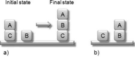
Case 4: this case measures the adaptation rate of the sensitivity to goal conflicts aspect of BNs. In this experiment we take into account the anoma-lous example situation of the block world (Sussman, 1975). In this classical conflicting-goals example there are three blocks (A, B, and C) which must be piled up in a specific order. The initial state of the world is S(0) =(\ clear-B., \clear-A., \A-on-C.) and the goals are G(0) = (\A-on-B., \B-on-C.). The robot should first achieve the goal \B-on-C.
and then the goal \A-on-B.. It is tempted, however, to immediately stack A onto B which may bring it into a deadlock situation (not want-ing to undo the goal already achieved). Some of the behaviors used for this experiment were: \stack-A-on-B., \stack-B-on-C., and \take-A-from-C.. See Figure 9.
Figure 6. Case 1: (a) the robot senses an orange box; (b) the robot activates\Pick-up-orange-box.behavior; (c) the robot senses other seven ‘‘green’’ boxes; (d) the robot does not change the attention focus even though it receives more activation from the situation (the seven green boxes). GBS = green box storage, OBS = orange box storage.
Figure 7. Case 2: (a) the robot reactively avoids a moving obstacle in front of it while it is carrying a box; (b) the robot finally stores the box in spite of multiple distracting obstacles.
only needed to adjust some parameters:p,g, andffor case 3;u,g, andffor case 2; andgandffor case 1.
Table 3 shows the statistical data from the experi-ments. The CE (convergence epoch) column indicates the mean epoch when the algorithm converged in every experiment. TheMSE is the mean square error for 100 runs of the corresponding experiment, where an error is considered as a wrong behavior activation produced in every execution step by the behavior network (in the
MSEgepcolumn the BN with the best fitness generated by the GEP algorithm is used and in theMSEmaes column the original Maes BN model without an evolutionary mechanism is used). TheMSE rate presents the perfor-mance relationship between MSEgep and MSEmaes. It is important to note that, for the experiments executed, the proposed evolutionary BN model improves the perfor-mance results obtained by the original Maes BN model by between 58% and 69%. This improvement is due to the capability of the proposed evolutionary BN model to self-adjust the global parameters in runtime, whereas the original Maes BN model was always restricted to a fixed configuration of these parameters.
For all the experiments, the original Maes BN model was configured with the following fixed global para-meters: d=90, g=50, f=90, p=90, and u=100. In contrast to these fixed values, Table 4 shows the global parameters discovered by the proposed evolutionary mechanism for each experimental case. From these results arise the following observations:
Case 1: the proposed evolutionary mechanism discov-ered that in order to keep the balance between the ‘‘goal-orientedness’’ and ‘‘situation-‘‘goal-orientedness’’ aspects,gmust be approximately 29–34% greater thanf. For a very high value ofgor a very low value off, the agent (robot) could not adaptively redirect its attention focus towards more interesting goals when they were presented.
On the other hand, a value offgreater thangwould prevent the robot achieving any of the goals because it would be continuously changing its attention focus.
Case 2: the proposed evolutionary mechanism found that in order to keep the balance between the ‘‘delibera-tion’’ versus ‘‘reactivity’’ aspects, the value offmust be a little higher thang(approximately 9–15%). With this con-figuration the agent was not only able to keep its attention
focused on current goals, but was also able to react against unexpected or dangerous situations. Additionally, when reactive behavior was required, the proposed evolutionary mechanism discovered that a low value ofuallowed fast behavior activation because the BN took fewer activation loops and, as a consequence, the amount of deliberative processing was considerably decreased.
Case 3: the proposed evolutionary mechanism revealed that in order to keep the balance between the ‘‘bias towards ongoing plans’’ versus ‘‘adaptivity’’ aspects, the value ofpmust be approximately 46–52% greater thang, and 72–77% less thanf. If these global parameters are kept between such ranges, the agent will not continually ‘‘jump’’ from goal to goal and in turn it will be able to adapt to changing situations. From the wrong solutions it is possible to infer that a value ofp
too much greater than g and f makes the BN more
adaptive, although less biased towards ongoing plans, hence the agent will continually be changing the current goals without keeping the focus on any of them.
Case 4: the proposed evolutionary mechanism discov-ered that in order to preserve the ‘‘sensitivity to goal con-flicts,’’ the value of d must be approximately 51–65% greater thang; if it is less than 50% greater the BN does not take away enough activation energy from conflicting goals. A value ofg greater thandcauses the BN to go into deadlock due to the inability of the BN to undo goals already achieved. Furthermore, the evolutionary mechanism found that the value off must be approxi-mately 62–73% greater thand, otherwise the BN will not be able to activate the behavior sequence that resolves
the goal conflict (i.e., \take-A-from-C., then
\stack-B-on-C., and then \stack-A-on-B.) because it will not receive enough activation from the observed state. Finally, the evolutionary mechanism revealed that in conflicting goal situations the value ofu
must be less thand, otherwise the BN will be more delib-erative and, therefore, it will execute more activation loops during which the behaviors that promise to directly achieve a goal (e.g.,\stack-B-on-C.and\ stack-A-on-B.) will accumulate more activation energy than those behaviors that solve conflictive goals through sub-goaling (e.g.,\take-A-from-C.).
From the results obtained in the above experiments, it is evident that setting global parameters is a ‘‘multi-objective’’ problem, hence a single BN solution cannot define a proper setting for all the proposed experimen-tal cases. So, the solution to this problem requires mul-tiple BNs competing for survival in the population, where only the best BN will be activated according to the situation observed by the agent.
5.3 Convergence rate of evolutionary
design of plans
In this experiment we proposed two different tasks that the robot had to accomplish. The first was the
box-collectingtask described in Section 5.1, and the sec-ond was a task in which the robot had to learn how to stack boxes on top of each other following specific order criteria (very similar to the Hanoi towers prob-lem). The basic idea of the problem is as follows: the robot has to collect different kinds of boxes (orange and green boxes), which are scattered everywhere, and to store them in the corresponding storage. The boxes
Figure 10. Behavior of the GEP population best and mean fitnesses during the evolutionary epochs for Cases 1, 2, 3, and 4.
Table 3. Statistics for BN functional evolution. CE is the convergence epoch of the curve.MSEgepis the mean square error of the case using the GEP algorithm.MSEmaesis theMSEusing only the original Maes BN model.MSErate is equivalent to
½1(MSEgep=MSEmaes).
Min. Max. Average SD CE MSEgep MSEmaes MSErate
Case 1 27 437 416.10 70.90 15 45.78 118.03 61.21% Case 2 35 472 455.44 69.10 9 41.39 98.36 57.91% Case 3 28 573 515.18 137.73 21 56.15 145.87 61.50% Case 4 53 683 629.01 143.98 27 73.02 233.28 68.69%
Table 4. Evolved global parameters.
d g φ p y
are piled up one on top of another in the same order that the robot finds them. After all boxes are stored, the robot has to stack, in an ordered manner, all the collected boxes in every storage.
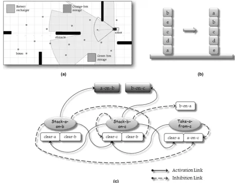
Figure 11a shows the environment used for the experiment. There were five green boxes (a, b, c, d, and e) and six orange boxes (f, g, h, i, j, and k). Figure 11b depicts an example where, given a set of stored boxes that were first stacked in a random order, the robot restacked them, this time following an ordered criteria (a-on-b, b-on-c, and so on).
Finally, Figure 11c depicts a partial segment of the BN for thebox-stackingtask. In our implementation we used variables for thebox-stackingBN, so the robot was able to reuse the behaviors in different situations. So, for example, ‘‘Stack-x-on-y’’ behavior receives two vari-ables (xandy) which can be any of the stored boxes.
The final aim of the experiment was that the robot had to generate a plan whose duration (in terms of exe-cution steps) was optimized. Thus, the robot had to minimize both the total number of execution steps nec-essary to collect all green and orange boxes, and the
number of execution steps to organize and stack (in an ordered manner) all the stored boxes.
It is important to note that both kinds of BNs used in this experiment were previously evolved by the robot with the purpose of focusing just on the planning prob-lem and speeding up the solution convergence. Additionally, before this experiment, the robot per-formed a training phase where it got specific knowledge about where every box and storage in the world was situated. Table 5 summarizes the GEP parameters used in the evolutionary process for generating plans.
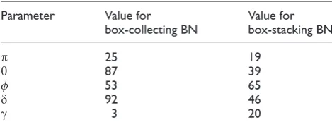
During the evolution of each ADF, the robot gener-ated two BNs with different structural and functional features. That make sense because, on the one hand, the BN for the box-collecting task needs: (1) to be more oriented to situations than to goals, that is, the behavior selection must be driven by what is happening in the environment; (2) to be more adaptable rather than biased to ongoing plans, so the robot can exploit new opportu-nities, be more fault tolerant, and adapt to dynamically changing situations such as the sudden need to recharge the battery because it has run out of energy, or the need
to replan because it finds a better solution in runtime; and (3) to be more deliberative (thoughtful) than reac-tive, because the robot has to plan all its movements towards whichever box and storage before starting mov-ing. On the other hand, the BN for box-stacking task requires: (1) to be more oriented to goals than to situa-tion because the environment is not affected by meaning-ful external changes while the robot is stacking the boxes; (2) to be more biased to ongoing plans rather than adap-table, so the robot can address behavior activation to the ongoing goals and subgoals of the task without a signifi-cant interference of external changes; (3) to be more sus-ceptible to avoiding goal and subgoal conflicts through the arbitration of behavior activation; and (4) to be more deliberative than reactive. All of these characteristics were evolved through the runtime adjustment (adapta-tion) of global parameters, as summarized in Table 6.
Note that in order to avoid very long plan simula-tions we used a simple criterion that prunes the space of simulations and improves the overall performance. So, we evaluated plans trivially: ‘‘at every epoch, all the plans are simulated concurrently using an independent processing thread for each plan; therefore, the first simulated plan to finish must be the route that takes least execution steps and time (duration) to traverse, and all the others could be aborted without loss.’’ Thus, in Figure 12 we only present the curve for the best plan found in every epoch.
Table 7 summarizes the statistical data from this
experiment. The error of MSE corresponds to every
plan whose fitness is negative after being evaluated by Equation 20 in every evolutionary epoch. Note that the best fitness reduces the MSE of the mean fitness curve by 64.38% (½1(MSEbest=MSEmean)).
Figure 12 shows the progress in time of the harmonic mean value for 100 runs of the best simulated plan (the one which took least execution steps to find a solution in every epoch). The robot found (on average) an optimized solution after epoch 400. In the plot, the harmonic mean value for the optimized solution converged at epoch 417 and took 576 execution steps. The optimized plan discov-ered by the evolutionary process is described next.
The homeotic gene (which is responsible for building deliberative plans as ordered-task sequences) uses two function nodes (T and D connectivity functions) and four terminal nodes that are connected to a specific ADF (ADF1, green-box-collecting BN; ADF2, orange-box-collecting BN; ADF3, stack-green-boxes BN; and
ADF4, stack-orange-boxes BN). Both ADF1 andADF2 receive a parameter in order to focus the spreading acti-vation dynamics of their corresponding BN. For exam-ple, if ADF1 received parametera, it would mean that
the BN would pursue the\store-a-box. subgoal;
if ADF2 received parameter f, it would mean that the
BN would pursue the\store-f-box.subgoal, and
so on. We can extract the corresponding plan as a sequence of ordered tasks obtained after applying the tree-traversal process in postorder on the ET of Figure 13, as follows:
Best Plan: [[ADF2:k] [ADF1:a] [ADF1:d] [ADF1:e] [ADF1:c] [ADF2:j] [ADF2:f] [ADF2:h] [ADF2:g] [ADF1:b] [ADF3] [ADF2:i] [ADF4]]
Translation:
Task 1: pick up ‘‘k’’ box and store it at orange storage
Task 2: pick up ‘‘a’’ box and store it at green storage
Task 3: pick up ‘‘d’’ box and store it at green storage
Task 4: pick up ‘‘e’’ box and store it at green storage
Task 5: pick up ‘‘c’’ box and store it at green storage
Task 6: pick up ‘‘j’’ box and store it at orange storage
Task 7: pick up ‘‘f’’ box and store it at orange storage
Table 5. GEP parameters for plans development (evolutionary process).
Parameter Value Parameter Value
Number of runs 50 Mutation rate 0.1 Number of generations (epochs) 500 One-point recombination rate 0.3 Population size (plans) 50 Two-point recombination rate 0.5 Number of ADFs 4 IS transposition rate 0.3 Number of homeotic genes 1 RIS transposition rate 0.3 Head length of homeotic gene 10
Table 6. Global parameters.
Parameter Value for box-collecting BN
Value for box-stacking BN
p 25 19
y 87 39
φ 53 65
d 92 46