Modeling a Multi-modal Distribution of Wind Direction Data in Kudat, Malaysia

Modeling a Multi-modal Distribution of

Wind Direction Data in Kudat, Malaysia

Nurulkamal Masseran

School of Mathematical Sciences, Faculty of Science and Technology Universiti Kebangsaan Malaysia, 43600 UKM Bangi, Selangor, Malaysia [email protected]

Abstract

Wind direction is the direction from which the wind is blowing. It is expressed in terms of degrees measured clockwise from geographical direction. The knowledge of the wind direction can be used to obtain information about the wind energy potential, dispersion of particulate matter in the air, the effects of engineering structures on the building, maritime study, and etc. This study provides a suitable model for the wind direction that indicates multi-modal distributional properties. A case study involves with a data from Kudat, Malaysia has been analysed. The statistical models known as a Finite Mixture of von Mises Fisher (mvMF) and Circular Distribution based on Nonnegative Trigonometric Sums (NNTS) has been fitted to the data. Then, the suitability of mvMF and NNTS models were judged based on a graphical representation and goodness-of-fit statistics. The results found that the mvMF model with H4 components is sufficient to provide a best model.

Keywords: Circular statistics, Dominant direction, Environmental statistics, Multi-modal distribution, Wind direction modelling.

1. Introduction

Wind direction is known as a type of circular or directional data. Thus, it has unique characteristics that are different from standard linear data sets. Such distinctive features have made directional statistics analysis substantially different from linear analysis (Mardia and Jupp, 1999; Masseran, 2015). Let



be a random variable that measures the directional data that take values in the range 0° to 360° or 0 to 2



. An analysis of



would depend on the selection of the starting point as the “zero-direction” and the sense of rotation. For example, in Figure 1, if the zero direction is due east, corresponding to anti-clockwise rotation, the data will take the value of 60°, whereas if the zero direction is due north, corresponding to clockwise rotation, the data will take the value of 30°. However, the "beginning" are always coincides with the "end", i.e., 0°-360°, and the measurement is also periodic, with  being the same as  p 2 for any integer p. The starting point and rotation from this point, regardless of whether it is clockwise or anticlockwise, are taken as positive values. Observations using these two dimensions are also called circular or directional data (Jammalamadaka and SenGupta, 2001).

In practice, the wind direction is an important feature that should be considered in building wind turbines and in structural and environmental design analysis. For that purpose, the statistical models always provide good information to describe about the behaviours of wind direction. In fact, the finite mixtures of von Mises distributions is among the most commonly used and was found to provide good results for the purpose of modelling the circular data, particularly for the wind direction. For examples, Masseran et al. (2013) showed that the finite mixture of the von Mises distribution with H number of components was the best distribution to describe the wind direction distributions in Malaysia. Carta et al. (2008) have showed that a the finite mixture of von Mises is a very flexible model for wind direction studies particularly for the wind direction regimes in zones with several models or prevailing wind directions. In fact, the same result have been showed by Azmani et al. (2009) in modelling the sensor data for the cases of a recursive change point estimate of the wind speed and direction. Apart from that, Heckenbergerova et al. (2015) showed that the finite mixture of von Mises distribution is able to provide an optimized solution for wind direction parameters corresponds to the Particle Swarm Optimization method. Thus, since the von Mises distribution is a flexible model for addressing wind directional data with several modes, this study attempts to describe and compare the suitability of von Mises model with the circular model based on nonnegative trigonometric sums in order to determine the best statistical model for wind direction data in Kudat.

2. Study area, data and descriptive statistics

Sabah is a state of Malaysia, located in the northern section of the island of Borneo (6.8833° N, 116.8333° E). It is the second largest state in the country after Sarawak, which it borders to the southwest. Sabah is relatively wet (annual precipitation exceeding 200 mm) due to the tail effect of typhoons, which frequently traverse the Philippine islands across the South China Sea. It is worth mentioning that from April to November each year, when typhoons frequently develop over the west Pacific and move westward across the Philippines, the south-westerly winds over the northwest coast of Sabah may reach speeds of 10.30 m/s or more (Masseran, 2013a).

The data used in this study were obtained from the Malaysian Meteorological Department. In this study, hourly wind direction data from 1 January 2009, to 30 November 2009 were used. Wind direction data are circular because they are recorded in terms of degrees, from 0° to 360°. However, for modelling, data transformation into radian units can be performed easily. Apart from that, the missing data has been estimated by using the method of single imputation (Masseran, 2013b).

the sample mean, also suffers from the same problem. Thus, we need an alternative measure of centre and dispersion when dealing with directional data (Jammalamadaka and SenGupta, 2001). Let  ₁, ₂ ,_n be a set of directional data; the mean direction can then be calculated as

 

 

 

 

1

1

1

tan , if 0, 0

, , if 0, 0

2

tan , if 0 1

tan 2 , if 0, 0

undefined , if 0, 0

S _{C S}

C

C S

S _C

C

S _{C S}

C

C S



 









 _{ }



 _{ }

 

_  



   



  



where,

1

cos

n i i

C 







and

1

S sin

n i i









accomplish the polar-to-rectangular transformation. On the other hand, the measure for the dispersion of the directional data is commonly derived from the circular variance, which is given as

 

2 2

1

1 2

V C S

n

  

A small value of the circular variance indicates the data have a large concentration around the mean direction.

The percentile measure for directional data is same as that for linear data: it is a measure of the value of a variable below a certain percent of observations. For example, the (100p)-th percentile is often called the quantile of order p. Let y1y2  yn be an order statistic for n observations; yr is then the quantile of order



1



r p

n



 as well as the



1001



r

n percentile. Thus, the p-th percentile of the data is also a quantile of order p for the

data. Using these descriptive measurements, Table 1 shows the descriptive statistics for the wind directional data in Kudat. Based on the descriptive statistics in Table 1, the circular mean of the wind direction is approximately 218.21°. However, the circular variance is 0.978, which implies that the data were not well concentrated around their mean direction. Thus, we suspect that the data are either approximately uniformly distributed or have a several-directional mean. The values of 25th, 50th, and 75th percentile

are 80°, 220°, and 240°, respectively.

3. Statistical models for the multi-modal distribution of circular data

to determine the best fitted model, the suitability of both of these models will be compare by using the Akaike’s Information Criterion (AIC) method.

3.1 Finite Mixture of von Mises-Fisher distributions (mvMF)

In some applications, the observed wind direction data cannot be represented by a unimodal distribution. To overcome this problem, a finite von Mises-Fisher mixture distribution (mvMF), which is comprised of a sum of H von Mises probability distributions, has been proposed. Let



_{be a random variable representing the wind} direction in radians, and let x'



cos_i,sin_i



' be a circular data point in rectangular coordinates. Then, the mixture of von Mises-Fisher distributions is given by









 

 ' 

 

1 1

; , ; , h h 3

H H

h h h h h h d h

h h

f   f   c  e

 









x μ

x μ x μ

where f



x μ; ,



c_d

 

 ex μ'  is a single von Mises Fisher model, d is a dimension of random vector

x

(in our cases d=2), μh,h are the parameter mean direction and concentration parameter, respectively, for h=1, 2,… H components of the von Mises distribution, while _h is a mixing parameter of nonnegative quantities that sum to one, given by





 

1

0 1 and 1 for 1, 2 , 4

H

h h

h

h H

 



 



 

 

d h

c



is a normalising constant given by

 

 

 

2 2

2

1

1

, 2

d d

d

h d h

h c

I  

 





 where I_r

 

.

represents the modified Bessel function of the first kind and order r. The MLEs for the mvMF are very difficult to derive in a standard way. However, Banerjee et al. (2005) provided a solution of the parameter estimates for the mvMF distribution based on the expectation maximisation (EM) approach. Let α_h 



μ_h,_h



denote the parameters of the von Mises-Fisher distribution, α_h 



μ_h,_h



, for 1 h H . Then, the mvMF distribution can be written as









 

1

; | 5

H

h h h h

f  f

  



x x α

where  



 ₁, ₁, ,_H,α α₁, ₂,,α_H



. According to Banerjee et al. (2005), to generate a random sample from this mixture distribution, the h-th von Mises distribution is randomly chosen with probability h. Let, X 



x x1, 2, ,xn



' be a data set of n independent sample points following Equation (17), and let Z 



z z₁, ₂, ,z_n



' be the corresponding set of hidden random variables that indicate a particular von Mises distribution from which a sample is generated. In particular, z_i h if x_i is generated from fh



x α| h



. Thus, the log-likelihood can be written as













 

1

ln , | ln | 6

i i i

H

z z i z i

f X Z  f



Assume that the posterior distribution, p h



|x_i,



, of the hidden variables Z|



X,



are known. Then, the expectation of the log-likelihood over the given posterior distribution p is given by













 















 















1 1 1

1 1 1 1

ln , | ln | 7

ln | | ,

ln | , ln | | ,

i i i

n

p p z z i z

i n H

h h i h i

i h

H n H n

h i h i h i

h i h i

E P X Z E f

f p h

p h f p h

                  _{ }      









x α

x α x

x x α x

Next, the parameter  _{is re-estimated to maximise the expectation function. To} maximise the expectation function with respect to _h, the Lagrangian multiplier  corresponding to the constraint

1 1 H h h   



is used, and by taking the partial derivatives with respect to each _h from the Lagrangian, the following is obtained:





 

1

| , 8

n

i h

i

p h 



  



x

Next, by summing both sides of Equation (20) over all h, Banerjee at al. (2005) found that  n; thus, the parameter estimate for _his given by





 

1

1

ˆ | , 9

n h i i p h n  





x Θ

The parameter estimates for α_h 



μ_h,



_h



can be derived under the constraints μ 1

and _h0 for h=1, 2, … H. Let _h be the Lagrange multiplier corresponding to the constraint; if  0, then f

 

x α| is the uniform distribution on the sphere, and if  0, then the multiplier for the inequality constraint has to be zero. Thus, the Lagrangian is given as

























 

















 

' 1

1 1 1

' '

1 1 1

, , ln | | , 1

ln | , | , 1 10

H n H

H

h h h h h i h i h h h

h i h

H n n

d h i h h i i h h h

h i i

L f p h

c p h p h

                    _      _  





 



μ x α x μ μ

x μ x x μ μ

By taking the partial derivative with respect to





1

, , H

h  h h _h

μ from Equation (22), and setting it equal to zero, for each h, Banerjee et al. (2005) obtained





 

1

| , 11

2

n h

h i i

i h p h    





μ x x

 

'

1 12

h h 

 

 









 

'

'

1 1

| , | , 13

n n

d h

i h i i

i i

d h c

p h p h

c 

  

   



x μ



x x

Using Equations (23) and (24), they found that



| ,



 

14

2

h

h ip h i



  x x 

and









 

1 1 | , 15 | , n i i i h n i i i p h p h     





x x μ x x

Next, substituting Equation (27) into Equation (25) provides the parameter estimates for h

 as given by

 

 









 

' 1 1 | , 16 | , n i i i d h n d h i i p h c c p h       





x x x

where













1

| | ,

| h h i

i k l l l f p h f       



x x x

. Readers desiring a detailed discussion of the

parameter estimates for the von Mises-Fisher distribution should consult (Banerjee et al., 2005; Hornik and Grun, 2014; Mooney et al., 2003).

3.2 Circular Distribution based on Nonnegative Trigonometric Sums (NNTS)

The NNTS model has been found to be flexible enough to model directional data sets exhibiting multimodality or skewness. The nonnegative trigonometric sum series for a circular variable  has been expressed by Fejer (1915) as the squared modulus of a sum of complex numbers, which can be written as

 

2

0

, for 0, 1, 2, , 17

M ik k k

c e  k M







where 2, i 1, and c_k is a complex parameter. Using this series, Fernandez-Duran [15] proposed a new family of distributions for circular random variables, given as





2  

 

0 0 0

; , i i 18

M M M

i k l x ikx

j k k l

k k l

f x M   e  e 

  









where the parameters



a_k,b_k



are expressed in terms of the complex parameter

0

2

n k

k k v k v

v

a ib c c

  

 



. An additional constraint, 2 ₀

0 1 2 n k k c a    

trigonometric sum integrate to 1. Thus, there are 2*M free parameters, where the parameter c₀ must be real and positive.

Next, to ensure that the integration for the probability density function is equal to one,



; ,



1

f M d

   



α , a constraint on the parameter  is needed, namely,

 

2

0

1

19 2

M k k



 





If  _c0 0 and  _rk 0, then _k is a non-negative real number. It then follows that Equation (3) can be written in the quadratic form



_j; ,



T _{j j}T

 

20

f  M α α e e α

where



2 3



'

1, ij, ij, ij, , Mij

j e e e e

   

   



e and _αT _{is a transposition and conjugate for vector}

α. Then, the likelihood function can be written as



1 2



 

1

, | , , 21

n

T T

n j j

k

L M   







α α e e α

and the log-likelihood function is derived as







1 2



 

1

ln , | , , 22

n

T T

n j j

k

L M   







α α e e α

To determine the maximum likelihood estimator for parameter , Fernandez-Duran & Gregorio-Dominguez (2010) suggested the application of the Newton-like manifold algorithm using the procedures described by Absil et al. (2008). Using the Newton-like manifold algorithm, the maximum likelihood estimator for the NNTS model can be solved by

 

 

23

gradl α 0

where gradl

 

α is a gradient for the log-likelihood function of the value of α in Equation (6). The solution of Equation (7) is the critical point of the real log-likelihood function for the NNTS model. The Newton-like manifold algorithm method provides the solution for the maximum likelihood estimator through several steps:

i) Determine the initial value for α₀

ii) For k0, 1, , solve the Newton equation, Hessl α_k η_k  gradl α_k for the

unknown η_k in the tangent space at α_k.

iii) Set αk1R

 

ηk , where R is a retraction from the tangent space onto the manifold at k

This algorithm terminates when the norm of the gradient or the norm of the difference

 

k

 

k1

 

 

 

1

1

24 2

T

n k

T T

k k

gradl P_ n

 



  



 

 

 



α e

α α

α α e

Apart from that, the NNTS model in Equation (2) can also be expressed as







 

 



 

1

1 1

; , cos sin 9

2

M

k k

k

f  M a k b k

  

 





α

where

0

2 _v

M k

k k v k

v

a ib  

  

 



for k 1, 2, ,M.

4. Results and discussion

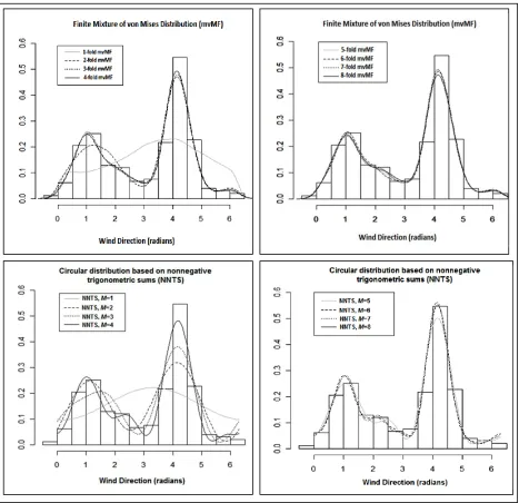
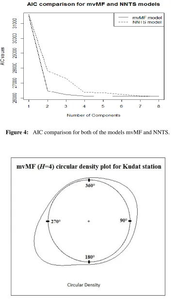
As mentioned above, the objective of this study was to identify the most appropriate distribution for wind direction at the Kudat station to better understand the wind regime in this area. Tables 2 and 3 show the parameter estimates for the mvMF and NNTS model respectively. Figure 3 presents the fitted mvMF and NNTS for the wind direction at the Kudat station. From the figure, it is clear that the single mvMF distribution (H=1) failed to model the wind direction data at the Kudat station accurately. The same conclusion is draw from NNTS model (M=1). However, as the number of components of the mvMF and NNTS model increase, both of the models fit the data in a more precise way. As a result, the fitted mvMF and NNTS models with 2, 3, …, 8 components model the data with similar accuracies. It is quite difficult to determine the suitability precision of both models based on graphical representations only. Thus, the Akaike’s Information Criterion (AIC) was used to evaluate the performance of both models.



 



 





 





 





 





 





 





 





  2 2 1 2 2 2 2 2 2 2 1 1 2 2 2 2 1 1 11.658 9.227 1 1 1 1 10.752 0.971 1 1 11.658

; , 0.3474064 0.1439757

2 11.658 2 9.227

10.752

0.1412261 0.3673919

2 10.752 2 0.971

9.227 0.971 d d T T d d d d d d T T d d d d

f e e

I I e e I I                 

μ x μ x

μ x μ x

x μ

with the parameter of mean directions,

1 2 3 4 0.56772170 0.8232205 -0.31381192 -0.9494852 -0.63765746 -0.7703200 0.02245815 0.9997478 T T                          μ μ μ μ .

Since the mvMF has been determined to be a good model for the data, it can be used to describe some characteristics of the wind direction in Kudat. In this study, the parameter

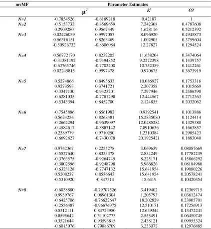
μ for mvMF has been defined in terms of rectangular coordinates. The interpretation of the dominant direction of the wind is not suitable to be described in this way. Thus, by transforming the results into units of degrees, 0  360 may be more appropriate. Based on Equation (31), the measured parameters for the mean directions in terms of degrees are 233.37°, 256.06°, 55.52° and 82.65°. In addition, Figure 5 shows a circular density plot for the mvMF with H=4 components. This figure clearly shows that most of the wind was blowing from the north-northeast and the west-southwest and some from the east-southeast. The circular density plot reveals that the wind direction has two different dominant directions: from 190°-270° with mean directions of 233.37° to 256.06° with respect to the parameter concentration  11.658 and 10.752, while the other dominant direction are found to be in the range of 30°-90° with mean directions of 55.52° and 82.65° and also the concentration parameter  9.227 and  0.971. These imply that a stronger concentration about the mean direction of the wind blow comes from the South-West direction and follow by the minor dominant direction of the wind blows from the North-East direction.

Apart from that, the others direction are found to be quite uniformly distributed. Determining the dominant wind direction will contribute valuable information to planning or forecasting activities in such sectors as wind energy generation, air pollution assessment, climate change, construction, and maritime activities. For example, in wind energy evaluation, based on this information, the wind turbine can be positioned such that the production of energy is maximised.

6. Conclusions

fact, it was found that mixtures von Mises-Fisher distributions with H4 components adequately modelled the wind direction distribution in Kudat. Apart from that, circular plots of the mvMF model clearly show that several wind directions are more dominant in Kudat, while the other directions show an approximately uniform dispersion.

Appendix

(a) Bessel Function and its Important Properties:

Bessel function, J_v

 

z for the order- vth, is a solution for the differential equation given by

2 2

2 2

1

1 0

x dx v

x z z dz z

 



  _{ } 

 _{ }

In addition, the Bessel function, J_v

 

z can also be written in term of the integration form given by

 

 

  



0 cos 2

1

2 _{sin ,}

1 1 2

2 2

iz v v

z

J z e d v

v   _{ }    _   _     



While in the the expansion series for Bessel function, J_v

 

z can be written as

 

 

 





2 0 2 1 ! 1 v r r v r z J z

r v r

       



For any positive integer n, the integration form of the Bessel function can also be written as

 





0 1 cos sin n

J z n z d



  









In fact, Jv

     

z  1 vJv z , dan



 



1

 

, 0

v v

v v

d

z J z z J z v

dz    .

In particular,

 









2 0 0 2 0 2 0 1 cos 2 1 cos cos 2 2 cos cos iz

J z e d

z d z d               







and d



zJ z₁

 



zJ₀

 

z

 

 

 





2 cos 0 2 0 1 cos 2 2 ! 1 v v v z v r r

I z i J iz

v e d z

r v r

              





In particular,

 

2 cos 0 0 1 2

I e d

  

 







has been determined as normalizing constant for the von Mises-Fisher distribution. The other properties of the modified Bessel function are explained based on the following Equations

 

 

 

 

'

 

1 1 , 2 , v v

v v v

I z I z

I z I z I z

     

 

 

 

 

 

 

1 1 '

0 0 1

2

,

,

v v v

v

I z I z I z

z d

I z I z I z

dz      

 

 



 

 



 

 

 

 

'' '

0 1 0 2

1 2 1 0 1 2

I z I z I z I z I z I z z I z I z z       

By referring to the above mentioned properties, it is found that d



I₁

 



I₀

 

, d     and d I1

 

I2

 

d          

  . Next, the properties of monotonic increasing function for the

parameter  in the Bessel function can be explain based on the ratio of

 

 

 

1 0 I A I    

with A'

 

 1 A

 

 A2

 

 . 

   Apart from that, some approximations for the Bessel function that having a small or large value of  can be solve using the following equations:

 



 





 









 

2 2 2

2

2 2 2

3

4 1 4 1 4 9

1 8

2 2 8

4 1 4 9 4 25

6 8 p

p p p

e I

p p p

 



 



 _{  } 

 

 _   _

 

 

  

 

In particular ₀

 

~ 2

e I





 , and

 

2

1 1

~ 1

2 8

A 

 

 _{  } 

 

 .

If  is small,

 

2 4

0 ~ 1 ,

4 64

I     and

 

2 4

~ 1

2 8 48

A  _    _

 .

For more detail regarding the properties of Bessel function, please refer to Jammalamadaka and SenGupta, 2001; Stephenson, 1973).

Acknowledgements

The authors are indebted to the staff of the Malaysian Meteorology Department for providing wind direction data. This research would not have been possible without sponsorship from the Ministry of Education, Malaysia (grant number: FRGS/1/2014/SG04/UKM/03/1 and GGPM-2014-056).

References

1. Mardia, K. V. and Jupp, P. E. (1999). Directional Statistics. John Wiley, Chichester.

2. Masseran, N. (2015). Markov chain model for the stochastic behaviors of wind-direction data. Energy Conversion and Management, 92; 266-274.

3. Jammalamadaka, S. R. and SenGupta, A. (2001). Topics in circular statistics. World Scientific Publishing, Singapore.

4. Fisher, N. I. (1993). Statistical analysis of circular data. Cambridge University Press, Cambridge.

5. Masseran, N., Razali, A. M., Ibrahim, K., and Latif, M. T. (2013). Fitting a mixture of von Mises distributions in order to model data on wind direction in Peninsular Malaysia. Energy Conversion and Management, 72: 94-102.

6. Carta, J. A., Bueno, C. and Ramirez, P. (2008). Statistical modelling of directional wind speeds using mixture of von Mises distributions: Case study. Energy Conversion and Management, 49: 897-907.

7. Azmani, M., Reboul, S., Choquel, J. B. and Benjelloun, M. (2009). A recursive, change point estimate of the wind speed and direction. IEEE 7th International Conference on Computational Cybernetics, Palma de Mallorca, Spain.

8. Heckenbergerova, J., Musilek, P. and Kromer, P. (2015). Optimization of wind direction distribution parameters using particle swarm optimization. Advances in Intelligent System and Computing, 334: 15-26.

Journal of Applied Sciences, Engineering and Technology, 6: 1774-1779.

10. Masseran, N., Razali, A. M., Ibrahim, K., Zaharim, A. and Sopian, K. (2013). Application of the single imputation method to estimate missing wind speed data in Malaysia. Research Journal of Applied Sciences, Engineering and Technology, 6: 1780-1784.

11. Banerjee, A., Dhillon, I. S., Ghosh, J. and Sra, S. (2005). Clustering on the unit Hypershere using von Mises-Fisher Distributions. Journal of Machine Learning Research, 6: 1345-1382.

12. Hornik, K. and Grun, B. (2014). movMF: An R package for fitting mixtures of von Mises-Fisher Distributions. Journal of Statistical Software 58: 1- 31.

13. Mooney, J. A, Helms, P. J. and Jolliffe, I. T. (2003). Fitting mixture of von Mises distributions: a case study involving sudden infant death syndrome. Computational Statistics & Data Analysis, 41: 505-513.

14. Fejer, L. (1915). Uber trigonometrische polynome. Journal fur die Riene und Angewandte Mathematik, 146: 53-82.

15. Fernandez-Duran, J. J. (2004). Circular distributions based on nonnegative trigonometric sums. Biometrics, 60: 499-503.

16. Fernandez-Duran, J. J. and Gregorio-Dominguez, M. M. (2010). Maximum likelihood estimation of nonnegative trigonometric sum models using a Newton-like algorithm on manifolds. Electronic Journal of Statistics, 4: 1402-1410. 17. Absil, P. A. Mahony, R. and Sepulchre, R. (2008). Optimization Algorithm on

Matrix Manifolds. Princeton University Press, Princeton.

Figure 1: The observed directional data depend on choice of origin and the sense of rotation [1].

Figure 2: Relationship between polar coordinate data (1, θ) and rectangular

Figure 4: AIC comparison for both of the models mvMF and NNTS.

Table 1: Descriptive statistics for Kudat wind direction

Kudat wind station

Mean direction 218.21° Circular variance 0.978

25th percentile 80° 50th percentile 220° 75th percentile 240°

Table 2: The parameter estimates for the mvMF model up to six numbers of components

mvMF Parameter Estimates

T

μ





N=1 -0.7854526 -0.6189218 0.42187 1

N=2 -0.5153732 -0.8569659 7.242308 0.4787608

0.2909280 0.9567449 1.628116 0.5212392

N=3 0.02426039 0.9997057 8.096920 0.4945873

0.56316151 0.8263469 1.002905 0.3759604

-0.50926732 -0.8606084 12.27827 0.1294524

N=4 0.56772170 0.8232205 11.658204 0.3474064

-0.31381192 -0.9494852 9.2272398 0.1439757

-0.63765746 -0.7703200 10.752359 0.1412261

0.02245815 0.9997478 0.970675 0.3673919

N=5 0.5274866 0.8495633 10.086927 0.1753316

0.9273593 0.3741721 2.207358 0.1015669

-0.3347130 -0.9423201 7.297946 0.2486590

-0.6281035 -0.7781298 12.444567 0.2712363

-0.5343394 0.8452700 2.124835 0.2032062

N=6 -0.7545886 0.6561982 0.9392541 0.1013886

0.5624254 0.8268481 15.2835080 0.1124414

-0.2662294 -0.9639097 12.0485284 0.1329380

-0.4584617 -0.8887142 7.8910636 0.1663857

0.2389779 0.9710250 1.2310384 0.2985423

-0.6692827 -0.7430078 20.1925421 0.1883040

N=7 0.9742367 0.2255278 3.069639 0.08087669

-0.5527640 0.8333378 2.834249 0.17782239

-0.3763575 -0.9264745 8.225171 0.15866292

-0.3802596 -0.9248798 5.966826 0.08184980

-0.6323128 -0.7747132 15.641954 0.19080226

0.5208237 0.8536643 15.641954 0.20578241

-0.5310920 -0.847314 15.6419 0.10420354

N=8 -0.6038800 -0.79707526 3.419402 0.12369715

0.9959767 0.08961304 1.205793 0.03612474

-0.6425706 -0.76622647 18.202829 0.23905701

-0.2556487 -0.96676975 12.510171 0.17256913

0.5312111 0.84723950 12.639344 0.13472241

0.8595642 0.51102773 2.555491 0.06450745

0.3521644 0.93593815 2.438121 0.09955324

Table 3: The parameter estimates for the NNTS model up to six numbers of components

NNTS Parameter Estimates

ˆ ˆ ˆ

k rk i ck

    ˆ_k ˆ_rk iˆ_ck

M=1 k=0; 0.39088770 + i(0.000) M=6 k=0; 0.33051696 + i(0.000)

k=1; -0.07851115 + i(0.01406219) k=1; -0.06448836 – i(0.0147715)

k=2; -0.08979539 – i(0.14949561)

M=2 k=0; 0.35145494 + i(0.000) k=3; 0.06867154 + i(0.00497386)

k=1; -0.07058781 + i(0.00018935) k=4; -0.05872581 + i(0.07351352)

k=2; -0.08954087- i(0.15044643) k=5; -0.00175609 – i(0.01752988)

k=6; 0.03374423 + i(0.00904722)

M=3 k=0; 0.34473199 + i(0.000)

k=1; -0.06519571 - i(0.01050682) M=7 k=0; 0.32966310 + i(0.000)

k=2; -0.08975569 – i(0.15251008) k=1; -0.06524948 - i(0.01568993)

k=3; 0.06761674 + i(0.00815430) k=2; -0.08992444 – i(0.15000096)

k=3; 0.06880256 + i (0.00497416)

M=4 k=0; 0.33206489 + i(0.000) k=4; -0.05858657 + i(0.07387359)

k=1; -0.06721701 - i(0.01422902) k=5; -0.00161553 – i (0.01720893)

k=2; -0.08899561 - i(0.15149014) k=6; 0.0339152 0+ i(0.00906594)

k=3; 0.06842034 + i(0.00487464) k=7; -0.01385732 - i (0.00392186)

k=4; -0.05831522 + i(0.07205559)

M=8 k=0; 0.32927979 + i(0.000)

M=5 k=0; 0.33191670 + i(0.000) k=1; -0.06543936 – i(0.01564708)

k=1; -0.06720818- i(0.01503347) k=2; -0.09033585 – i(0.14995585)

k=2; -0.08942703 – i (0.15065709) k=3; 0.06905995 + i(0.00473962)

k=3; 0.06766157 + i(0.00499270) k=4; -0.05825125 + i(0.07392021)

k=4; -0.05874579 + i(0.07219662) k=5; -0.00165490 – i(0.01733769)

k=5; -0.00101357 – i(0.01676556) k=6; 0.03366950 + i(0.00892418)

k=7; -0.01402637 – i(0.00393321)

k=8; 0.00447990 – i(0.01254067)

Table 4: AIC values for comparison between mvMF model and NNTS model

Model AIC Model AIC

mvMF (H=1) 31472.46 NNTS (M=1) 31576.27

mvMF (H=2) 26468.94 NNTS (M=2) 27811.47

mvMF (H=3) 26231.88 NNTS (M=3) 27311.61

mvMF (H=4) 26141.58 NNTS (M=4) 26368.29

mvMF (H=5) 26123.57 NNTS (M=5) 26356.16

mvMF (H=6) 26113.17 NNTS (M=6) 26239.38

mvMF (H=7) 26111.30 NNTS (M=7) 26135.64