for the Parameters of the Power Function Distribution
Azam Zaka
Punjab Education Department Lahore, Pakistan
Ahmad Saeed Akhter
College of Statistical & Actuarial Sciences University of the Punjab, Lahore, Pakistan [email protected]
Abstract
This paper is concerned with the modifications of maximum likelihood, moments and percentile estimators of the two parameter Power function distribution. Sampling behavior of the estimators is indicated by Monte Carlo simulation. For some combinations of parameter values, some of the modified estimators appear better than the traditional maximum likelihood, moments and percentile estimators with respect to bias, mean square error and total deviation.
Keywords: Parameter estimation, Percentile estimators, Maximum likelihood estimators, Moment estimators, Modified estimators, Monte Carlo study, Total deviation, Mean square error.
1. Introduction
The Power function distribution is a flexible life time distribution model that may offer a good fit to some sets of failure data. Theoretically Power function distribution is the inverse of Pareto distribution. An excellent account of this distribution and its properties is given in Kleiber and Kotz (1970). Meniconi and Barry (1995) discussed the application of Power function distribution. They proved that the Power function distribution is the best distribution to check the reliability of any electrical component. They used Exponential distribution, Lognornal distribution and Weibull distribution and showed from reliability and hazard function that Power function distribution is the best distribution.
The probability distribution of Power function distribution is
( ) (1) With shape parameter and scale parameter , the interval (0, )
Cohen and Whitten (1982) used the moment and Modified Moment Estimators for the Weibull Distribution. Samia and Mohammad (1993) used five modifications of moments to estimate the parameters of the Pareto Distribution. Lalitha and Anand (1996) used Modified Maximum Likelihood to estimate the scale parameter of the Rayleigh Distribution. Rafiq (1996) discussed the parameters of the Gamma Distribution. Rafiq (1999) discussed the method of Fractional Moments to estimate the parameters of Weibull Distribution. Kang and Young (1997) estimated the parameters of a Pareto Distribution by Jackknife and Bootstrap Methods. Neil (2005) estimated the parameters of Weibull Distribution with the help of percentiles. He called it Common Percentile Method. Zaka and Akhter (2013) derived the different estimation methods for the parameters of Power function distribution. Zaka and Akhter (2013) discussed the different modifications of the parameter estimation methods and proved that the modified estimators appear better than the traditional maximum likelihood, moments and percentile estimators.
In this paper, we use the percentiles method, maximum likelihood and moment method to estimate the two parameters of the Power function distribution. The present paper introduces the modified estimators for parameters of the Power function distribution. The resulting estimators are easier to calculate than the maximum likelihood and, for certain combinations of parameter values; they improve the estimated values and mean square error. We examine these methods using two parameters Power function distribution to find the most accurate method (the method which has least M.S.E).
2. Methodology
2.1. Percentile Estimator (P.E)
Let be a random sample of size n drawn from probability density function of Power function distribution. The cumulative distribution function for a Power function distribution with shape and scale parameters , respectively
( ) . / (2)
By solving we get
( ) ⁄ (3)
Where = ( )
Let P75 and P25 are used.
( )
( ) ⁄ (4)
Dividing (4) and (5) we get
(
) (
)
(
) (
)
̂ .
/
. /
̂
( ) ⁄̂
̂ . /
( ) (6)
̂
( ) ⁄̂ (7)
Where H+L = 1.
2.2. First Modified Percentile Estimator (M.P.E.1)
In this modification of the percentile estimators, equation (5) is replaced by the coefficient of variation of Power function distribution.
√ ( ) (8)
and ( ) ⁄ (4)
From (8)
̅ √ ( )
Taking square in both sides we get
(
̅) ( )
( ) ( ̅)
Simplification we get
̂ √ ̅ (9)
̂
( ) ( √ ⁄ ̅ ) ̂
( ) ( √
̅ ) ⁄
(10)
2.3. Second Modified Percentile Estimator (M.P.E.2)
In this modification of the percentile estimators, equation (5) is replaced by the median of Power function distribution.
̃
⁄
i.e. ̂ ̃ ⁄ (11)
From (4) ̂ ( ) ⁄
̃ ⁄ ( ) ⁄
( ) ⁄
̃
Taking ln on both sides ⁄ ( ) = ln( ̃ )
̂ ( ) (
̃ )
̂ ( )
( ̃) (12)
2.4. Third Modified Percentile Estimator (M.P.E.3)
Using E ( ( )) = ( ) of Power function distribution and ( ), by neglecting( ).
( ) ⁄ (4)
̂
( ) ⁄ (13)
And E ( ( )) = ( ) (14)
(
( )
)
( )
(
)
⁄
Equating (13) and (15)
( ) ⁄ ( )( ) ⁄
( ) ( ( )) ⁄
ln (
( )) ( ( ))
⁄
ln (
( )) ⁄ , ( (
̂ = ( ( ))
(
( ))
̂ = ( ( ))
(
( ))
(16)
2.5. Maximum Likelihood Method (M.L.E)
Let be a random sample of size n drawn from probability density function of Power function distribution. The likelihood function of this random sample is the joint density of the n random variables and is a function of the unknown parameters. Thus
( )
Likelihood function is
( ) ∏ ( )
( ) ∏
∑
( )
The maximum likelihood estimator (MLE) of the parameter is the value of the parameter that maximizes L and MLE for 2 parameter of Power function distribution can be obtained by solving the equations resulting from setting the two partial derivatives of L( , ) to zero;
(17)
Where tn is the largest value in the sample data.
∑ ( ) (19)
̂ ( ( ) ∑
) (20)
2.6. First Modified Maximum Likelihood Estimator (M.M.L.E.1)
By neglecting (17) and replacing
E ( ( )) = ( )
.
( )
/
( )
(
)
⁄
̂ ( )( ) ⁄ (21)
Put in (19) we get
∑
. ( )( ) ⁄ /
∑
{ ( ) ( )}
( ) ( ) ∑
* ( )+ ( ) ∑
̂ * ( )+ ( ) ∑
̂ * ( )+
( ) ∑ (22)
2.7. Second Modified Maximum Likelihood Estimator (M.M.L.E. 2)
From equation (17) and (19)
( ) (23)
Replacing (23) by median of Power function distribution
̃
⁄
i.e ̂ ̃ ⁄ (25)
Put in (24) ∑ . ̃ ⁄ /
∑
{ ( ̃) ( )}
( ) ( ̃) ∑
* ( )+= ( ̃) ∑
̂ * ( )+ ( ̃) ∑
̂ [ * ( )+
( ̃) ∑ ] (26)
2.8. Third Modified Maximum Likelihood Estimator (M.M.L.E.3)
Using c.v of Power function distribution and neglecting
∑ ( ) (19)
√ ( ) (27)
̅ √ ( )
̂ √ ̅ (28)
Where is standard deviation and ̅ is mean.
∑
( )
( ) ∑
( ) ∑
̂
{∑
}
2.9. Moment Estimators (M.E)
The method of moments is another technique commonly used in the field of estimation of parameters. If the numbers represent a set of data, then an unbiased estimator for the kth origin moment is
∑
Where stands for thr kth sample moment.
The first moment of Power function distribution is
( ) ∫ ( )
( ) ∫ (
)
( ) ∫
( ) (
)
( )
And ( ) ∫ .
/
( ) ∫ ( )
( ) ∫
( )
Therefore by equating sample and population moments we get
́ ( )
(30)
And ́ = ( )
From (30) ̅
̅( )
̂ ̅( ) (32)
Put in (31), we get
̅ ( ) ( )
̅ ( )
( )
( ) ̅ ;
Where and ̅
̅ ̅ ( ) ( ) ( ̅ ) ( ) ̅ ( )
̅ ̅ ̅ ̅ ̅
̅
̅
̅
̂ √ ̅ (33)
2.10. First Modified Moment Estimator (M.M.E.1)
In this modification of the moment estimators, the second moment of two parameters Power function distribution is replaced by the coefficient of variation of Power function distribution.
√ ( ) (34)
(30)
Taking square in both sides we get
(
̅) ( )
( ) ( ̅)
Simplification we get
̂ √ ̅ (35)
2.11. Second Modified Moment Estimator (M.M.E.2)
In this modification of the moment estimators, the second moment of two parameters Power function distribution is replaced by the variance of Power function distribution.
i.e.
( )( ) (36)
and
(30)
( ) ̂ ( )( ) ̅
( ) ( )( )
̅
Where ̅
Therefore ̅
̂ √ ̅ (37)
and ̂ ( ̂ )( ̂ ) ̅ (38)
2.12. Third Modified Moment Estimator (M.M.E.3)
In this modification of the moment estimators, the first moment of two parameters Power function distribution is replaced by the variance of Power function distribution.
i.e.
( )( ) (36)
( ) ( )( )
̂ ( ̂ )√( ̂⁄ )
( ) ( )( )
( ) ( )
̅ ( )
̅
( )
̅ ( )
̅
̅
̂ √ ̅ (39)
̂ ( ̂ )√( ̂⁄ ) (40)
2.13. Fourth Modified Moment Estimator (M.M.E.4)
Using co-efficient of variation of Power function distribution and , by neglecting .
(31)
√ ( ) (34)
From (31) ( )
( ) ( ) ̅
̂ √ ̅ (41)
Three approximations for ̂( ) based on its being uniformly distributed on interval [0, 1] show in Table.
Method F(ti)
(a) MEDIAN RANK
(b) MEAN RANK
(c) SYMMETRICAL CDF
Methods for estimating F(ti)
3. Performance Indices (Goodness of Fit Analysis)
Some methods of goodness of fit analysis are employed here. Mean square error MSE and total deviation TD are two measurements that give an indication of the accuracy of parameter estimation. AL-Fawzan (2000) referred to the use of the procedure of MSE and TD.
3.1. Mean Square Errors (MSE)
The MSE can be calculated as below
Standard bias, Bias = E ( ̂) – and M.S.E ( ̂) = 0( ̂ – ) 1
Standard bias, Bias = E ( ̂) – and M.S.E ( ̂) = 0( ̂ – ) 1
3.2. Total Derivation (TD)
The total derivation TD, calculated for each method is as follows
| ̂ | | ̂ |
Where and are the known parameters, and ̂ n ̂ are the estimated parameters by any method. These techniques are used to measure the variability of parameter estimates for each simulation. These are used to determine the overall “best” parameter estimation method.
4. Application
the 2-parameters Power function distribution using different sample sizes and different values of parameters with mean square error MSE and total deviation TD.
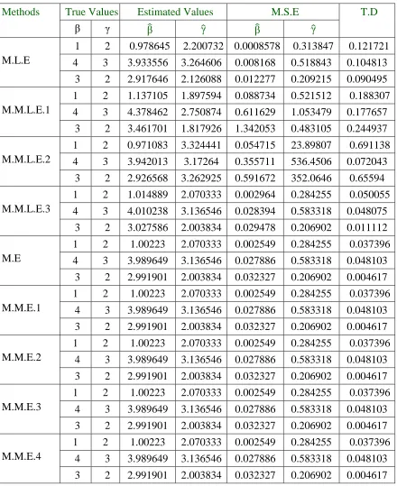
Table 1: (Comparison between maximum likelihood, moments and modified estimators for the parameters β and γ of Power function distribution under the sample size 20)
Methods True Values Estimated Values M.S.E T.D
̂ ̂ ̂ ̂
M.L.E
1 2 0.978645 2.200732 0.0008578 0.313847 0.121721
4 3 3.933556 3.264606 0.008168 0.518843 0.104813
3 2 2.917646 2.126088 0.012277 0.209215 0.090495
M.M.L.E.1
1 2 1.137105 1.897594 0.088734 0.521512 0.188307
4 3 4.378462 2.750874 0.611629 1.053479 0.177657
3 2 3.461701 1.817926 1.342053 0.483105 0.244937
M.M.L.E.2
1 2 0.971083 3.324441 0.054715 23.89807 0.691138
4 3 3.942013 3.17264 0.355711 536.4506 0.072043
3 2 2.926568 3.262925 0.591672 352.0646 0.65594
M.M.L.E.3
1 2 1.014889 2.070333 0.002964 0.284255 0.050055
4 3 4.010238 3.136546 0.028394 0.583318 0.048075
3 2 3.027586 2.003834 0.029478 0.206902 0.011112
M.E
1 2 1.00223 2.070333 0.002549 0.284255 0.037396
4 3 3.989649 3.136546 0.027886 0.583318 0.048103
3 2 2.991901 2.003834 0.032327 0.206902 0.004617
M.M.E.1
1 2 1.00223 2.070333 0.002549 0.284255 0.037396
4 3 3.989649 3.136546 0.027886 0.583318 0.048103
3 2 2.991901 2.003834 0.032327 0.206902 0.004617
M.M.E.2
1 2 1.00223 2.070333 0.002549 0.284255 0.037396
4 3 3.989649 3.136546 0.027886 0.583318 0.048103
3 2 2.991901 2.003834 0.032327 0.206902 0.004617
M.M.E.3
1 2 1.00223 2.070333 0.002549 0.284255 0.037396
4 3 3.989649 3.136546 0.027886 0.583318 0.048103
3 2 2.991901 2.003834 0.032327 0.206902 0.004617
M.M.E.4
1 2 1.00223 2.070333 0.002549 0.284255 0.037396
4 3 3.989649 3.136546 0.027886 0.583318 0.048103
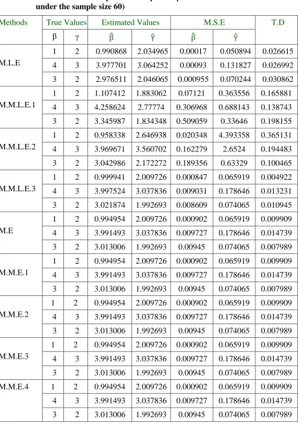
Table 2: (Comparison between maximum likelihood, moments and modified estimators for the parameters β and γ of Power function distribution under the sample size 60)
Methods True Values Estimated Values M.S.E T.D
̂ ̂ ̂ ̂
M.L.E
1 2 0.990868 2.034965 0.00017 0.050894 0.026615
4 3 3.977701 3.064252 0.00093 0.131827 0.026992
3 2 2.976511 2.046065 0.000955 0.070244 0.030862
M.M.L.E.1
1 2 1.107412 1.883062 0.07121 0.363556 0.165881
4 3 4.258624 2.77774 0.306968 0.688143 0.138743
3 2 3.345987 1.834348 0.509059 0.33646 0.198155
M.M.L.E.2
1 2 0.958338 2.646938 0.020348 4.393358 0.365131
4 3 3.969671 3.560702 0.162279 2.6524 0.194483
3 2 3.042986 2.172272 0.189356 0.63329 0.100465
M.M.L.E.3
1 2 0.999941 2.009726 0.000847 0.065919 0.004922
4 3 3.997524 3.037836 0.009031 0.178646 0.013231
3 2 3.021874 1.992693 0.008609 0.074065 0.010945
M.E
1 2 0.994954 2.009726 0.000902 0.065919 0.009909
4 3 3.991493 3.037836 0.009727 0.178646 0.014739
3 2 3.013006 1.992693 0.00945 0.074065 0.007989
M.M.E.1
1 2 0.994954 2.009726 0.000902 0.065919 0.009909
4 3 3.991493 3.037836 0.009727 0.178646 0.014739
3 2 3.013006 1.992693 0.00945 0.074065 0.007989
M.M.E.2
1 2 0.994954 2.009726 0.000902 0.065919 0.009909
4 3 3.991493 3.037836 0.009727 0.178646 0.014739
3 2 3.013006 1.992693 0.00945 0.074065 0.007989
M.M.E.3
1 2 0.994954 2.009726 0.000902 0.065919 0.009909
4 3 3.991493 3.037836 0.009727 0.178646 0.014739
3 2 3.013006 1.992693 0.00945 0.074065 0.007989
M.M.E.4 1 2 0.994954 2.009726 0.000902 0.065919 0.009909
4 3 3.991493 3.037836 0.009727 0.178646 0.014739
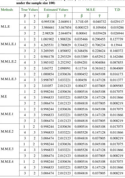
Table 3: (Comparison between maximum likelihood, moments and modified estimators for the parameters β and γ of Power function distribution under the sample size 100)
Methods True Values Estimated Values M.S.E T.D
̂ ̂ ̂ ̂
M.L.E
1 2 0.995338 2.048911 3.71E-05 0.040732 0.029117
4 3 3.986661 3.047854 0.000323 0.109404 0.019286
3 2 2.98528 2.044074 0.00041 0.039428 0.026944
M.M.L.E.1
1 2 1.081902 1.908326 0.035466 0.290455 0.127739
4 3 4.265531 2.780829 0.334422 0.706234 0.13944
3 2 3.269395 1.858852 0.348456 0.228624 0.160372
M.M.L.E.2
1 2 0.984178 2.293329 0.013389 0.652912 0.162486
4 3 3.985102 3.252392 0.094201 0.904084 0.087855
3 2 3.04372 2.098991 0.11714 0.361612 0.064069
M.M.L.E.3
1 2 1.000854 2.030636 0.000452 0.045108 0.016173
4 3 3.998787 3.033221 0.00458 0.147128 0.011377
3 2 3.01057 2.012123 0.00437 0.037805 0.009585
M.E
1 2 0.998244 2.030636 0.000516 0.045108 0.017075
4 3 3.996833 3.033221 0.005528 0.147128 0.011866
3 2 3.006474 2.012123 0.004818 0.037805 0.008219
M.M.E.1
1 2 0.998244 2.030636 0.000516 0.045108 0.017075
4 3 3.996833 3.033221 0.005528 0.147128 0.011866
3 2 3.006474 2.012123 0.004818 0.037805 0.008219
M.M.E.2
1 2 0.998244 2.030636 0.000516 0.045108 0.017075
4 3 3.996833 3.033221 0.005528 0.147128 0.011866
3 2 3.006474 2.012123 0.004818 0.037805 0.008219
M.M.E.3
1 2 0.998244 2.030636 0.000516 0.045108 0.017075
4 3 3.996833 3.033221 0.005528 0.147128 0.011866
3 2 3.006474 2.012123 0.004818 0.037805 0.008219
M.M.E.4 1 2 0.998244 2.030636 0.000516 0.045108 0.017075
4 3 3.996833 3.033221 0.005528 0.147128 0.011866
Table 4: (Comparison between percentile estimators and modified percentile estimators for the parameters β and γ of Power function distribution under the sample size 20)
Methods True Values Estimated Values M.S.E T.D
̂ ̂ ̂ ̂
P.E(5,95) 1 2 0.963314 1.914608 0.000842 0.336271 0.049109
4 3 3.93834 2.68987 0.006584 0.79654 0.099876
3 2 3.05117 2.51692 0.009876 0.33698 0.096325
M.P.E.1(5 , 95) 1 2 1.006413 1.94920 0.0005443 0.34987 0.052698
4 3 4.009277 2.790714 0.004107 0.64841 0.072081
3 2 3.003777 1.828275 0.005991 0.288481 0.087121
M.P.E.2(5 , 95) 1 2 0.962884 1.98285 0.009865 0.31587 0.069878
4 3 3.90627 4.70869 0.008954 0.87598 1.00258
3 2 3.05623 2.32768 1.02356 0.44569 0.99987
M.P.E.3(5 , 95) 1 2 0.955534 2.81742 0.02568 0.69874 0.08974
4 3 3.99683 1.51702 0.36547 0.89547 1.12547
3 2 3.05095 2.52579 0.12458 1.02365 0.09999
P.E(25,75)
1 2 1.02118 1.94920 0.0067588 0.399743 0.037396
4 3 4.033476 2.68987 0.05474 0.746732 0.012429
3 2 3.06322 2.51692 0.056018 0.502218 0.01792
M.P.E.1(25 ,75)
1 2 1.014671 2.028446 0.002549 0.284255 0.028894
4 3 4.14214 2.987819 0.027886 0.583318 0.048103
3 2 3.014928 2.025889 0.032327 0.206902 0.004617
M.P.E.2(25 ,75)
1 2 1.06012 1.55491 0.002549 0.284255 0.037396
4 3 3.99252 4.10038 0.027886 0.583318 0.048103
3 2 3.11731 2.18263 0.032327 0.206902 0.004617
M.P.E.3(25 ,75)
1 2 0.977914 2.75832 0.002549 0.284255 0.037396
4 3 4.55513 1.42423 0.027886 0.583318 0.048103
Table 5: (Comparison between percentile estimators and modified percentile estimators for the parameters β and γ of Power function distribution under the sample size 60)
Methods True Values Estimated Values M.S.E T.D
̂ ̂ ̂ ̂
P.E(5,95)
1 2 1.00362 2.020935 0.07121 0.134476 0.011973
4 3 4.01174 3.36567 0.306968 0.688143 0.138743
3 2 3.03379 1.67547 0.509059 0.33646 0.198155
M.P.E.1(5 , 95) 1 2 1.001506 2.11504 0.000234 0.363556 0.165881
4 3 4.002723 2.945079 0.0015 0.293768 0.018988
3 2 3.006631 1.932092 0.001793 0.133337 0.036164
M.P.E.2(5 , 95) 1 2 1.01130 1.60909 0.020348 4.393358 0.365131
4 3 4.04036 2.29499 0.162279 2.6524 0.194483
3 2 3.02366 1.88107 0.189356 0.63329 0.100465
M.P.E.3(5 , 95) 1 2 1.00519 1.98730 0.000847 0.065919 0.004922
4 3 4.01585 3.15379 0.009031 0.178646 0.013231
3 2 3.04060 1.56118 0.008609 0.339364 0.010945
P.E(25,75)
1 2 0.987804 1.949088 0.002205 0.163036 0.029359
4 3 3.93727 3.36567 0.016628 0.339364 0.014739
3 2 3.18543 1.67547 0.022423 0.163036 0.007989
M.P.E.1(25 ,75)
1 2 1.003903 2.11504 0.000902 0.065919 0.009909
4 3 3.997267 3.031052 0.009727 0.178646 0.011034
3 2 3.019546 2.019861 0.00945 0.074065 0.016446
M.P.E.2(25 ,75)
1 2 1.04515 1.49485 0.000902 0.065919 0.009909
4 3 4.13844 2.12615 0.009727 0.178646 0.014739
3 2 3.20107 1.62901 0.00945 0.074065 0.007989
M.P.E.3(25 ,75)
1 2 0.995826 1.99633 0.000902 0.065919 0.009909
4 3 3.95577 3.19068 0.009727 0.178646 0.014739
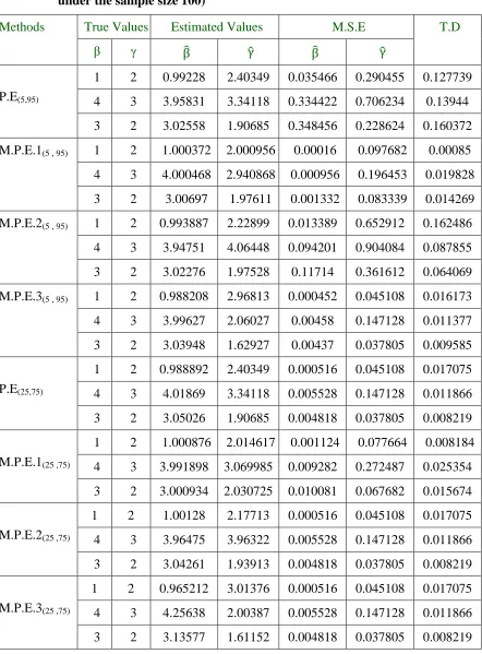
Table 6: (Comparison between percentile estimators and modified percentile estimators for the parameters β and γ of Power function distribution under the sample size 100)
Methods True Values Estimated Values M.S.E T.D
̂ ̂ ̂ ̂
P.E(5,95)
1 2 0.99228 2.40349 0.035466 0.290455 0.127739
4 3 3.95831 3.34118 0.334422 0.706234 0.13944
3 2 3.02558 1.90685 0.348456 0.228624 0.160372
M.P.E.1(5 , 95) 1 2 1.000372 2.000956 0.00016 0.097682 0.00085
4 3 4.000468 2.940868 0.000956 0.196453 0.019828
3 2 3.00697 1.97611 0.001332 0.083339 0.014269
M.P.E.2(5 , 95) 1 2 0.993887 2.22899 0.013389 0.652912 0.162486
4 3 3.94751 4.06448 0.094201 0.904084 0.087855
3 2 3.02276 1.97528 0.11714 0.361612 0.064069
M.P.E.3(5 , 95) 1 2 0.988208 2.96813 0.000452 0.045108 0.016173
4 3 3.99627 2.06027 0.00458 0.147128 0.011377
3 2 3.03948 1.62927 0.00437 0.037805 0.009585
P.E(25,75)
1 2 0.988892 2.40349 0.000516 0.045108 0.017075
4 3 4.01869 3.34118 0.005528 0.147128 0.011866
3 2 3.05026 1.90685 0.004818 0.037805 0.008219
M.P.E.1(25 ,75)
1 2 1.000876 2.014617 0.001124 0.077664 0.008184
4 3 3.991898 3.069985 0.009282 0.272487 0.025354
3 2 3.000934 2.030725 0.010081 0.067682 0.015674
M.P.E.2(25 ,75)
1 2 1.00128 2.17713 0.000516 0.045108 0.017075
4 3 3.96475 3.96322 0.005528 0.147128 0.011866
3 2 3.04261 1.93913 0.004818 0.037805 0.008219
M.P.E.3(25 ,75)
1 2 0.965212 3.01376 0.000516 0.045108 0.017075
4 3 4.25638 2.00387 0.005528 0.147128 0.011866
5. Conclusions
All the results are listed in tables 1 to 6. A Monte Carlo simulation study shows that if we compare the M.L.E, M.E and their modifications, we find that for small sample size their modified estimators produce better results. But as the sample size increases than only M.L.E provides best results. M.E does not show any reliable results.
If we compare the Percentile estimators (P.E) and its modifications then we see that for small sample size the Modified percentile estimators (M.P.E) and in some cases Percentile estimators (P.E) produce the best results for and . The estimated values of and are close to their true values. But as the sample size increases the only M.P.E.1 (First Modified Percentile Estimator) provides the best estimators (the method which has least M.S.E).
Among all the Percentile estimators and their modifications, P (5, 25) produces best results,
which shows that larger data produce better results. The best estimator among all the Percentile estimators and Modified percentile estimators is M.P.E.1 (5, 95).
Finally, we recommend using M.P.E.1 and M.L.E modifications methods for small sample size and only M.L.E when the sample size is large.
It is very interesting that the result of M.E and its modifications are equal but their formulae are different.
References
1. Ahsanullah, M. and Kabir, L. (1975). Estimation of the location and scale parameters of a Power function distribution by linear functions of order statistics.
Communications in Statistics, 5, 463-467.
2. Al-Fawzan, M. A. (2000). Algorithms for Estimating the Parameters of the Weibull Distribution, King Abdul-Aziz City for Science and Technology, Riyadh, Saudi Arabia.
3. Cohen, A. C. and Whitten, B. J. (1982). Estimation in the three parameters Lognormal Distribution. Journal of the American Statistical Association, 75, 399-404.
4. Kang, S.B. and Young, C.S. (1997). Estimation of the Parameters in a Pareto Distribution by Jackknife and Bootstrap Methods. Journal of Information and Optimization Science, 18, 289-300.
5. Lalitha, S. and Anand, M. (1996). Modified Maximum Likelihood Estimators for Rayleigh Distribution. Communication in Statistics: Theory and Method, 25(2), 389-401.
6. Lwin, T. (1972). Estimation of the tail of Paretian Law.
Skandinaviskaktuarietiidskrift, 55, 170-178.
8. Meniconi, M. and Barry, M. D. (1995). The Power function distribution: A useful and simple Distribution to assess Electrical Component Reliability.
Microelectronics Reliability, 36(9), 1207-1212.
9. Neil, M. (2005). Estimation of Weibull parameters from common percentiles.
Journal of applied Statistics, 32, 17-24.
10. Pablo, B.S. and Bruce, E.R. (1992). Model Parameter Estimation using Least Squares. Water Research, 26(6), 789-796.
11. Rafiq (1996). Estimation of parameters of the Gamma Distribution by the method of fractional moments. Pakistan Journal of Statistics, 12(3), 265-274.
12. Rafiq (1999). Estimation of parameters of the Weibull Distribution by the method of Fractional Moments. Pakistan Journal of Statistics, 15(2), 91-96.
13. Rider, P. R. (1964). Distribution of the product, quotient of maximum values in samples from a Power function population. Journal of the American Statistical Association, 59, 877-880.
14. Ronald, E.W. and Raymond, H. M. (1978). Probability and Statistics for Engineers and Scientists (2nded). McMillan Publishing Co., Inc., New York. 15. Samia, A. S. and Mohammad M. M. (1993). Modified Moment Estimators for
three parameters Pareto Distribution. Institute of Statistical Studies and Research,
Cairo University, 28 (2).
16. Zaka, A. and Akhter, A. S. (2013). Methods for estimating the parameters of the Power function distribution. Pakistan Journal of Statistics and Operational Research, 9(2), 213-224.