ESTIMATION OF PARAMETERS IN A PLANAR SEGMENT PROCESS WITH A BIOLOGICAL APPLICATION

ESTIMATION OF PARAMETERS IN A PLANAR SEGMENT PROCESS

WITH A BIOLOGICAL APPLICATION

VIKTOR

BENE

ˇ

B

JAKUB

VE

ˇ

ˇ

BENJAMIN

ELTZNER

_CARINA

_WOLLNIK

FLORIAN

REHFELDT

_VERONIKA

_KR

_´

_´

_STEPHAN

_HUCKEMANN

1_{Charles University, Faculty of Mathematics and Physics, Department of Probability and Mathematical}

Statistics, Sokolovsk´a 83, 18675 Praha 8, Czech Republic ;2Georg-August-University of G¨ottingen, Institute of Mathematical Stochastics, Goldschmidtstrasse 7, 37077 G¨ottingen, Germany;3Georg-August-University of G¨ottingen, Third Institute of Physics - Biophysics, Friedrich-Hund-Platz 1, 37077 G¨ottingen, Germany e-mail: [email protected], [email protected], [email protected],

[email protected], [email protected], [email protected], [email protected]

(Received September 18, 2016; revised November 17, 2016; accepted November 30, 2016)

ABSTRACT

The paper deals with modeling of segment systems in a bounded planar set (a cell) by means of random segment processes. Two models with a density with respect to the Poisson process are presented. In model I interactions are given by the number of intersections, model II includes the length distribution and takes into account distances from the centre of the cell. The estimation of parameters of the models is suggested based on Takacz-Fiksel method. The method is tested first using simulated data. Further the real data from fluorescence imaging of stress fibres in mesenchymal human stem cells are evaluated. We apply model II which is inhomogeneous. The degree-of-fit testing of the model using various characteristics yields quite satisfactory results.

Keywords: parameter estimation, random segment process, stem cell, stress fibre.

INTRODUCTION

In stochastic geometry (Chiuet al., 2013) random geometrical objects and their systems are studied. The basic model is a stationary spatial point process on the whole Euclidean space. Sometimes, however, a stochastic model in a bounded set is needed, e.g. in the biological example investigated in this paper. We will study the distribution of actin stress fibres in individual stem cells. The goal is to model this system for each cell by means of a finite point process (Møller and Waagepetersen, 2007; Baddeley, 2007) including marks which leads to a segment process (Chiuet al., 2013; Pawlas, 2014).

The goal of our present paper splits into two aims. First we develop background theory of segment processes. Particularly we are interested in parameter estimation in models given by a density with respect to the Poisson process (Møller and Waagepetersen, 2004). For systems of objects the disc process case was developed in Møller and Helisova (2008; 2010), the facet process in Veˇceˇra and Beneˇs (2016); Veˇceˇra (2016), where facets are compact subsets of hyperplanes in Rd. Because of

problems with normalizing constant the Takacz-Fiksel

method or maximum pseudolikelihood method are suitable choices, cf. Coeurjolly et al. (2012) for spatial point processes and Dereudre et al. (2014) for disc processes. The applicability of the Takacz-Fiksel method is first successfully tested on simulated data. The simulation of a realization of a finite segment process is obtained by means of the birth-death Metropolis-Hastings algorithm of Markov chain Monte Carlo (Geyer and Møller, 1994).

MATERIALS AND METHODS

In many applications, systems of randomly dispersed segments in the plane or space are investigated. In biology, such systems occur e. g. when using fluorescence imaging to observe stress fibres in stem cells. Real data from an ongoing research consists of actin stress fibres in human mesenchymal stem cells (hMSCs) taken from the bone marrow. In the experiment, stem cells have been cultured on gels of different stiffness for 24 hours. This stiffness is given in terms of the Young’s modulus, the ratio of stress by strain, i.e. the force per area needed to deform the material.

Earlier experiments have found that hMSCs can be mechanically guided to differentiate towards various cell types depending on the substrate elasticity they are grown on, namely neuron precursor cells for 1 kPa, muscle precursor cells for 10 kPa and bone precursor cells for 30 kPa (Engler et al., 2006). Especially the differentiation into neuron precursor cells is remarkable, since hMSC stem from the mesodermal tissue layer, while neurons are ectodermal cells. It has also been found that these three populations of cells on different gels express significantly disparate fibre patterns after 24 hours on the gel, (Zemelet al., 2010). It is therefore interesting to closely examine the stress fibre patterns especially for cells on a gel with 1 kPa stiffness. In the present paper we investigate group G1 ofn1=138 cells which corresponds to a Young’s modulus of 1 kPa and it is mostly suitable for a simple stochastic modeling.

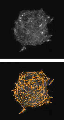
Using the Filament Sensor algorithm (Eltzner et al., 2016) it is possible to transform the raw data into a system of segments. Fig. 1 shows an example cell and the automatic line detection result. The corresponding segment systems of each cell are characterized by the following geometrical parameters:

– cell shape,

– spatial distribution of segments,

– length distribution,

– directional distribution.

In the following we suggest a methodology of quantitative description of these attributes.

Fig. 1.Cell 12 on 1 kPa gel, original microscopy image (upper image) and microscopy image overlayed with fibers (lower image) detected by the Filament Sensor (Eltzner et al., 2016).

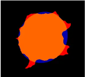
DESCRIPTION OF THE CELL SHAPE

Fig. 2.The shape of cell 12 on 1 kPa gel as detected by the Filament Sensor (Eltzner et al., 2016) compared to the elliptical approximation.

SPATIAL POINT PROCESS GIVEN BY A DENSITY

Consider a bounded measurable planar setB⊂R2

of area|B|>0 and a measurable space(N,N)of finite point subsets ofB.HereNis the space of outcomes and N a system of measurable subsets ofN,see Baddeley (2007) for more details. A random element having values in(N,N) is called a finite point process. Let a Poisson point processη on B have finite intensity

measureλ(mean number of points in a given subset of B) and probability distributionP_η onN.We consider a finite point processµ onBgiven by a density pwith

respect toPη,i. e. with distributionPµ

dPµ(x) =p(x)dPη(x),x∈N, (1)

wherep:N→R+is measurable satisfying

Z

N

p(x)dP_η(x) =1.

For a measurable mapF:N→R,F(µ) is a random

variable. The distribution of the process is alternatively determined by the conditional intensity,

λ∗(x,u) = p(x∪u)

p(x) ,

whereλ∗(x,u)|du|is interpreted as the probability that there is a point of the process in a small neighbourhood du of u given that the process is equal to x outside du. An important tool is the Georgii-Nguyen-Zessin formula

E

"

∑

u∈µ

q(u,µ\ {u}) #

= Z

BE

[λ∗(µ,u)q(u,µ)]du,

(2) valid for any measurable test functionqonB×N.

THE SEGMENT PROCESS WITH REFERENCE DIRECTIONAL DISTRIBUTION

LetB⊂R2be as above, let[0,π)be the semicircle

of axial directions, and put

Y =B×[0,π). (3)

A segmentx= (s,φ)∈Y has centresand directionφ

(we will assume for simplicity a fixed segment length r>0 here).

Consider a measurable space (M,M) of finite point sets in Y. A random element having values in

(M,M)is called a finite segment process.

We deal with the Poisson segment process η(s)

with the intensity measureλ onY,where

λ(d(y,φ)) = s πdydφ

for a constants>0.Let the segment processXhave a density pw.r.t.η(1),we consider model I:

p(x) =cexp(a N(x))zn(x)

_∏

x_i∈x

g(φi), (4)

with parametersa≤0,z>0,the normalizing constant c,the statisticsn(x) (the total number of segments in x), N(x) (the total number of intersections between segments in x). Finally φi is the direction of i−th segmentxi andg is a reference probability density on [0,π).The conditional intensity corresponding to the

density pin (4) is foru= (y,φ),u∈/x,

λ∗(x,u) =zg(φ)exp(aNx(u)),

whereN_x(u)is the number of segments fromxwhich hit u.The Metropolis-Hastings birth-death algorithm for simulating a realization of the segment process X is that of Geyer and Møller (1994) where the Hastings ratio for birth is

H(x,u) =exp(aNx(u))

zg(φ)|B|

(n(x) +1)

and the proposal density is uniform onY.

Example:Let the directional densityg be that of von Mises distribution on [0,π) with parametersκ ≥

0, ν ∈R,which is suitable for unimodal distribution

(νis the mode andκreflects the concentration around ν):

d(κ) =_πI1

0(κ),I0(κ)is the modified Bessel function of the first class and order 0. Then

p(x) =c(θ)exp(hθ,G(x)i), x∈M, (5)

whereh., .iis the scalar product,

θ= (a,log(zd(κ)),κ),

G(x) = (N(x),n(x),

_∑

x_i∈x

cos(2(φi−ν))),

segmentsxi= (si,φi)have centressi∈Band directions

φi∈[0,π).The normalizing constantc(θ)is defined as

c(θ) =R 1

exp{hθ,G(x)i}dP_η(1)(x)

.

Also

{θ∈R3:

Z

exp{hθ,G(x)i}dP_η(1)(x)<∞}

is the largest set of θ such that the density (Eq. 5) is well defined. It is the exponential class density (Møller and Waagepetersen, 2004) where classical maximum likelihood estimation (MLE) or Bayesian estimation of parameters are available, but they depend on an unknown normalizing constant, which may cause computational problems.

PARAMETER ESTIMATION, MODEL I

We will demonstrate the Takacz-Fiksel method of parameter estimation in the above model (Eq. 5). From the Georgii-Nguyen-Zessin formula (Eq. 2) we obtain the so called innovation

∑

u∈X

q(u,X\u)− Z

Y

λ∗(X,u)q(u,X)du

which is a centered random variable. Using suitable test functions q and setting innovations equal to zero leads to a system of equations for unknown parametersκ,a,zgiven thatrandνare known. These

latter parameters are observable, the lengthr directly, the dominant direction ν by the methods of mode

estimation. The asymptotic properties of this estimator are studied in Coeurjolly et al. (2012). We use test functionsNx(u),cos(2(φ−ν)),1,respectively, where

u= (y,φ).Dividing the first two equations by the third

one we obtain a system of two equations for unknown a,κ:

1

n(x)_u

∑

∑Ji=1b(a,κ,x,ui)Nx(ui)

∑Ji=1b(a,κ,x,ui)

,

1

n(x)_u

∑

=∑ J

i=1b(a,κ,x,ui)(cos(2(φi−ν)))

∑J_i=1b(a,κ,x,ui)

,

where

b(a,κ,x,ui) =exp(aNx(ui) +κcos(2(φi−ν))).

On the left hand side of the equations we have statistics of the data x. Integrals on the right hand side are approximated by sums, using simulations of additional segments ui = (yi,φi), i=1, . . . ,J, of fixed length r from the uniform distribution on Y. Having solved (numerically) the above system of two equations we estimate the third parameterzas

z= |B|

n(x)I0(κ)J

J

∑

i=1

b(a,κ,x,ui)

!−1

.

THE SEGMENT PROCESS WITH REFERENCE LENGTH DISTRIBUTION

Next we extend the previous model by dealing also with a random segment length. The shape of the window and the location of segments take into account the intended biological application. Consider an ellipse B⊂R2 centred in the origin, with axes lengthse1≥ e2>0 and area|B|=πe1e2/4. LetLo= (0,e1]be the interval of possible segment lengths, then

Y =B×Lo×[0,π) (6)

is the space of segmentsu= (s,r,φ)which have centre

s,lengthr=l(u)and axial directionφ.

Let the Poisson segment process η(s) have the

intensity measureλ onY of the form

λ(d(y,r,φ)) = s

e₁πdydrdφ

for a constants>0.Let the segment processX have a density pwith respect toη(1),model II:

p(x) =c1[x⊂B]exp(b D(x))zn(x)

∏

ri

e1

, (7)

with parametersb>0,z>0,n(x)is the total number of segments inx,cis the normalizing constant,riis the length ofi−th segmentxi,gis a reference probability density onLoand

D(x) =

_∑

d(u), d(u) =max w∈u

||w|| e₁ .

the centre of the cell. The corresponding conditional intensity is

λ∗(x,u) =1[x∪u⊂B]zg

r e1

exp(bd(u)).

Example:We use the reference length densitygof the beta distribution with parametersα,β >0

g(r) =r

α−1_(1−r)β−1

B(α,β) , r∈(0,1),

with the beta function in the denominator. It is a natural unimodal distribution where two parameters enable the shift of the mode along the interval and also flexibility of the variance.

PARAMETER ESTIMATION, MODEL II

For the parameter estimation we suggest again the Takacz-Fiksel method. The parameters e1,e2 are known as described in the subsection on cell shape. Using four test functions

d(u), log(l(u)

e₁ ), log(1− l(u)

e₁ ), 1,

and dividing the equations corresponding to the first three test functions by the equation corresponding to the fourth test function we obtain the system of three equations for unknownb,α,β:

D(x)

n(x) =

∑Ji=1exp(bd(ui))g(_eri

1)d(ui) ∑Ji=1exp(bd(ui))g(_eri

1)

,

∑u∈xlog(l(u))

n(x) =

∑Ji=1exp(bd(ui))g(_eri

1)log(ri) ∑Ji=1exp(bd(ui))g(_eri

1)

,

∑u∈xlog(e1−l(u)) n(x) =

=∑ J

i=1exp(bd(ui))g(_eri

1)log(e1−ri) ∑Ji=1exp(bd(ui))g(_eri

1)

,

and finally we put the estimators of b,α,β in the equation forz:

z= Mn(x)

|B|∑Ji=1exp(bd(ui))g(_eri

1)

.

The segments ui = (yi,ri,φi) are generated from the uniform distribution onY,i=1, . . . ,M and onlyJ of them which lie completely inBare used.

TESTING OF THE FIT OF THE MODEL

Once we have estimated parameters of the model from the data, it is necessary to test whether the model

fits the data well. Monte Carlo tests are common in spatial statistics, which are based on some scalar or functional test statistics of the data pattern (Møller and Waagepetersen, 2004). Then we simulate realizations of the model based on estimated parameters, and find upper and lower limits of values of estimated test statistics. In the case of test functions the envelopes formed by pointwise minima and maxima are plotted and it is evaluated how well the test function estimated from the data falls between the envelopes. Various designs of these methods are developed in Myllym¨aki et al.(2015).

In the present paper we restrict ourselves to scalar test statistics. LetTi,i=1, . . . ,n,be a random sample of a statisticT,

Tl=min(T1, . . . ,Tn), Tu=max(T1, . . . ,Tn), (8)

obtained from independent simulations of the model with estimated parameters, and ˆT is the observed value from the data. If Tˆ > Tu or Tˆ < Tl we reject the hypothesis that the data come from the model. The significance level is unknown since the testing procedure is not independent of the estimation procedure. Using the double Monte Carlo procedure from Dao and Genton (2014) it is possible to avoid this problem and reach the prescribed significance level which is computationally demanding.

Consider the null hypothesis that the segment directions a1, . . . ,an come from uniform directional distribution. Alternative hypothesis says that this is not the case. Axial data come from the interval [0,180]

in degrees. Let a₍₁₎≤a₍₂₎≤ · · · ≤a_(n)be the ordered sample. Evaluate

Vn= max i=1,...,n

_a (i) 180− i n − min

i=1,...,n

_a (i) 180− i n +1 n (9) and the modified Kuiper’s test statistic (Mardia and Jupp, 1999) is

V(x) =Vn

_√

n+0.155+0√.24 n

. (10)

Critical values for the test are tabulated, but dataxfrom a single cell are not independent, therefore also here the Monte-Carlo approach described above has to be used. Having in mind that model II is isotropic on a circle, we consider the data xc transformed from the elliptic cell shape onto a circle Bc by means of new planar coordinates

x0=e2

e1

x, y0=y. (11)

RESULTS

SIMULATION RESULTS

For a numerical demonstration of the Takacz-Fiksel method we simulated n = 100 realizations of the segment process on [0,1]2 of both model I (with parameters ν = π/2,z = 1000,a = −3,κ =

1,r = 0.06) and model II (with parameters e₁ =

e2 =1,z=100,b=0.5,α =3,β =3). Finding all

intersections of a segment system is a problem from computational geometry. One can use the Bentley-Ottmann algorithm, (Bentley and Bentley-Ottmann, 1979). In Fig.3 we demonstrate how model I depends on the interaction parametera.The Takacz-Fiksel estimators of(a,z,κ)(model I) and of(z,b,α,β)(model II) were

evaluated withJ=1000 for each realization. Empirical means and standard deviations (sd) of the estimators are printed in Table 1. It should be mentioned that in practice we have typically a single realization, while here we simulate one hundred independent realizations.

Fig. 3. Simulated realizations of model I segment processes on [0,1]2 _{with parameters}

ν = π/2,z =

1000,κ =1,r =0.06, in the upper pattern we have a=−0.6 and statistics n(x) =624,N(x) = 204. In the lower pattern we have a=−3 (more repulsion) and statistics n(x) =433,N(x) =5.

Table 1.Means and standard deviations (sd) of Takacz-Fiksel estimates from 100 simulations on [0,1]2 of model I (with observable parameters µ =π/2,r =

0.06) and model II (with e1=e2=1). The true values of estimated parameters are in the table.

Model I true mean sd

a -3 -2.998 0.299

κ 1 0.999 0.078

z 1000 1008.9 64.2

Model II true mean sd

b 0.5 0.525 0.463

α 3 3.089 0.296

β 3 3.147 0.458

z 100 104.32 40.25

REAL DATA RESULTS

In Fig. 4 there are twenty cells from groupG1 for further analysis. Those cells were selected which fit the ellipsoidal shape best. The cell numbers and the relative amount of pixels outside the ellipse are given in Table 2.

Table 2.Shape description: the numbers of cells from group G1 investigated and their area outside ellipse (AOE) in percent of pixels.

1 2 5

6 18 19

20 30 31

34 43 49

55 59 60

64 92 93

127 131

Fig. 4. Analysed segment systems corresponding to stress fibres in cells from group G1and their numbers. The shape of the cell is approximated by ellipse with axes lengths in Table 3.

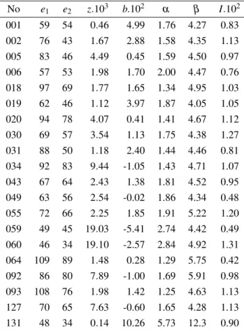
The selected cells were then fitted to the model II with reference length distribution. The estimated parameter values are in the Table 3.

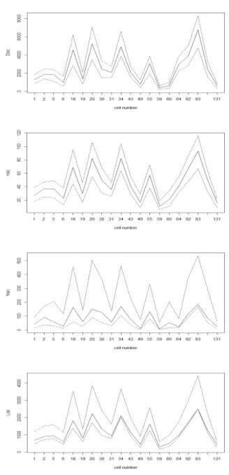
The test of the fit of the model II is based on scalar test statisticsn(x),D(x)from the model and moreover onN(x),L(x),the total number of intersections, total length of segments, respectively. In Fig. 5 the results from n=20 simulations are presented for each cell. The bounds (8) are plotted by dashed lines and the values of the test statistic from real data lie between the bounds in all cases. For the test statisticsn(x),D(x)

from the model naturally the fit is better and the line corresponding to data lies almost in the middle of the bounds. We summarize that based on the selected statistics we cannot reject the hypothesis of model compatibility for any cell. To obtain the level of our test is computationally demanding as explained above.

Finally we used the modified Kuiper’s statistics (10) to the transformed dataxcin (11) and the result is in Fig. 6. For one cell the test statistic lies outside the interval and in this case we reject the null hypothesis.

Table 3. The results of the Takacz-Fiksel estimator with reference beta length distribution, model II. The columns involve subsequently: the cell number, the axes lengths e1,e2(in pixels, where 1 pixel=0.32µm),

estimated parameters z,b,α,β and the ratio I= _en(x)

1e2 which is proportional to number density of segments.

No e1 e2 z.103 b.102 α β I.102

001 59 54 0.46 4.99 1.76 4.27 0.83 002 76 43 1.67 2.88 1.58 4.35 1.13 005 83 46 4.49 0.45 1.59 4.50 0.97 006 57 53 1.98 1.70 2.00 4.47 0.76 018 97 69 1.77 1.65 1.34 4.95 1.03 019 62 46 1.12 3.97 1.87 4.05 1.05 020 94 78 4.07 0.41 1.41 4.67 1.12 030 69 57 3.54 1.13 1.75 4.38 1.27 031 88 50 1.18 2.40 1.44 4.46 0.81 034 92 83 9.44 -1.05 1.43 4.71 1.07 043 67 64 2.43 1.38 1.81 4.52 0.95 049 63 56 2.54 -0.02 1.86 4.34 0.48 055 72 66 2.25 1.85 1.91 5.22 1.20 059 49 45 19.03 -5.41 2.74 4.42 0.49 060 46 34 19.10 -2.57 2.84 4.92 1.31 064 109 89 1.48 0.28 1.29 5.75 0.42 092 86 80 7.89 -1.00 1.69 5.91 0.98 093 108 76 1.98 1.42 1.25 4.63 1.13 127 70 65 7.63 -0.60 1.65 4.28 1.13 131 48 34 0.14 10.26 5.73 12.3 0.90

Fig. 6. The result of testing the uniformity of directional distribution for the dataxc transformed to a circle. The full line corresponds to V(xc),cf. (10), the bounds (8) are based on 20 simulations of the model on a circle with parameters estimated from transformed data. Cell 19 is omitted since the estimator has not been achieved, for the cell 93 we observe that V(xc)

does not lie between the bounds which leads to the rejection of null hypothesis.

DISCUSSION

As written in the Introduction, the paper has two aims, a mathematical and an applied one. The segment process having a density with respect to the Poisson process and reference directional and/or length distributions presents a new model for segment systems on a bounded set which may posses interactions. More complex models can be built by using joint direction-length distribution models, but in fact model II is of this kind where the directional distribution is uniform. It should be mentioned that generally the reference distribution need not coincide with the observed distribution. The model I is a Gibbs type homogeneous process while model II is an inhomogeneous Poisson process. We suggested the parameter estimator based on Takacz-Fiksel method for both models, the estimating equations were solved numerically using the Nelder-Mead method. First we showed the capabilities of the estimation procedure in simulated segment systems.

Model I was introduced for simulation and demonstration purposes, because of its homogeneity it arised not to be useful for the modeling of real data from hMSCs. Theferore we tried to apply the model II to real data of stress fibres observed by fluorescence imaging and transformed into segment systems. In model II we involve a special statistics D(x) which performs quite well. The negative values of the corresponding parameter b for cells 34,49,59,60,92,127 (cf. Table 3) correspond to a uniform distribution of short filaments across the cell or even tendency to cluster around the centre. Positive values in other cases correspond to a typical accumulation more close to the boundary than to the centre of the cell. The beta distribution of the length is also stable in parameters α,β (with the

exception of cell 131). Positive results of the degree-of-fit test in Fig.5 do not yet mean that the data completely correspond to the model since the test is conservative. Moreover functional characteristics (like the contact distribution function) could be implemented as descriptors of spatial distribution. Nevertheless all the presented arguments together make the model II interesting and valuable for the underlying biological problem.

ACKNOWLEDGEMENT

REFERENCES

Baddeley A (2007). Spatial point processes and their applications. In: Weil W ed. Stochastic geometry. Lect Not Math 1892:1–75.

Bentley JL, Ottmann TA (1979). Algorithms for reporting and counting geometric intersections. IEEE Transac Comput C28(9):643-47.

Chiu B, Stoyan D, Kendall WS, Mecke J (2013). Stochastic Geometry and Its Applications. 3rd Ed. New York: Wiley.

Coeurjolly JF, Dereudre D, Drouilhet R, Lavancier F (2012). Takacs-Fiksel Method for Stationary Marked Gibbs Point Processes. Scand J Statist 39:416–43.

Dao A, Genton, MG (2014). A Monte Carlo adjusted goodness-of-fit test for parametric models describing spatial point patterns. J Comput Graph Statist 23:497– 517.

Dereudre D, Lavancier F, Helisova K (2014). Estimation of the intensity parameter of the germ-grain Quermass-interaction model when the number of germs is not observed. Scand J Statist 41:809–29.

Eltzner B, Wollnik C, Gottschlich C, Huckemann S, and Rehfeldt F (2016). The filament sensor for near real-time detection of cytoskeletal fiber structures. PLOS ONE 10(5):e0126346.

Engler AJ, Sen S, Sweeney HL, Discher DE (2006). Matrix elasticity directs stem cell lineage specification. Cell 126(4):677–89.

Geyer CJ, Møller J (1994). Simulation procedures and likelihood inference for spatial point processes. Scand J Statist 21:359–73.

Mardia KV, Jupp PE (1999). Directional Statistics. New York: Wiley.

Møller J, Helisova K (2008). Power diagrams and interaction process for unions of discs. Adv Appl Probab 40:321–47.

Møller J, Helisova K (2010). Likelihood inference for unions of interacting discs. Scand J Statist 37:365–81. Møller J, Waagepetersen R (2004). Statistical Inference and

Simulation for Spatial Point Processes. Singapore: CRC Press.

Møller J, Waagepetersen R (2007). Modern Statistics for Spatial Point Processes. Scand J Statist 34:643-84. Myllym¨aki M, Grabarnik P, Seijo H, Stoyan D (2015).

Deviation test construction and power comparison for marked spatial point patterns. Spat Statist 11:19–34. Pawlas, Z (2014). Self-crossing points of a line segment

process. Method Comput Appl Probab 16:295–309. Veˇceˇra J, Beneˇs V (2016). Interaction processes for unions

of facets, the asymptotic behaviour with increasing intensity. Method Comput Appl Probab 18(4):1217–39. Veˇceˇra J (2016). Central limit theorem for Gibbsian U-statistics of facet processes. Appl Math 61(4):423–41. Zemel A, Rehfeldt F, Brown AEX, Discher DE, Safran