An Optimization Framework for “Build-or-Buy” Strategy for component Selection in a Fault Tolerant Modular Software System under Recovery Block Scheme

Ratio Mathematica, 21, 2011, pp. 91-105

91

An Optimization Framework for “Build-or-Buy”

Strategy for component Selection in a Fault Tolerant

Modular Software System under Recovery Block Scheme

P.C.Jha* Ritu Arora** U.Dinesh Kumar***

*Department of Operational Research , University of Delhi,India **Maharaja Agrasen Institute of Technology, GGSIP University, Delhi,India.

***Indian Institute of Management, Bangalore, India *[email protected] ** [email protected] ***[email protected]

Abstract

This paper discusses a framework that helps developers to decide whether to buy or build components of software architecture. Two optimization models have been proposed. First model is Bi-criteria optimization model based on decision variables in order to maximize the software reliability with simultaneous minimization of the overall cost of the system. The second optimization model deals with the issue of compatibility.

Keywords : Modular software, software reliability, software cost, fault tolerance, software components, recovery block scheme

1. Introduction

92

software failures is through fault tolerance. One way to reduce the risks of software design faults and thus enhance software dependability is to use software fault tolerance techniques. Software fault tolerance techniques are employed during the procurement, or development, of the software. They enable a system to tolerate software faults remaining in the system after its development. When a fault occurs, these techniques provide mechanisms to the software system to prevent system failure from occurring. There are two structural methodologies for Fault Tolerant System i.e. Recovery Block Scheme and N-Version Scheme. In this paper, we will discuss optimization model for recovery block. Non functional aspects play a significant role in determining software quality. Given the fact that lack of proper handling of non functional aspects (Cysneiros et al, [5]) of a software application has led to a series of software failures, nonfunctional attributes such as reliability security and performance should be considered during the component selection phase of software development. This paper discusses a framework that helps developers to decide whether buying or building components of software architecture on the base of cost and non functional factors. While developing software, components can be both bought as COTS (Commercial Off-The Shelf) products, and probably adapted to work in the software system, or they can be developed in-house. This decision is known as “build-or-buy decision”. This decision affects the overall cost and reliability of the system. Most of today’s software systems include one or more COTS products. COTS are pieces of software that can be reused by software projects to build new systems. Benefits of COTS based development include significant reduction in the development cost, time and improvement in the dependability requirement. No changes are normally made to their source codes. COTS components are used without any code modification and inspection. The components, which are not available in the market or cannot be purchased economically, can be developed within the organization and are known as in-house built components. Kapur et al [8] discussed issues related to reliability of systems through weighted maximization of system quality subject to budgetary constraint.

93

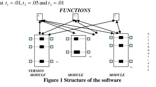
alternative and only one version will be selected for each alternative of a module. If a component is in-house build component, then the alternative of a module is selected. A schematic representation of the software system is given in Figure 1. We are selecting the components for modules to maximize the system reliability by simultaneously minimizing the cost. The frequency with which the functions are used is not same for all of them and not all the modules are called during the execution of a function, the software has in its menu. Software whose failure can have bad effects afterwards can be made fault tolerant through redundancy at module level (Belli and Jadrzejowicz, [1]). We assume that functionally equivalent and independently developed alternatives (i.e In-house or COTS) for each module are available with an estimated reliability and cost. The first optimization model (optimization model-I) of this paper maximizes the system reliability with simultaneously minimizing the cost. The model contains four problems (P1), (P2), (P3) and (P4). Problem (P1) is not in normalized form, therefore, it has been normalized and transformed into problem (P3) and (P4). The second optimization model (optimization model-II) considers the issue of compatibility between different alternatives of modules as it is observed that some COTS components cannot integrate with all the alternatives of another module. The models discussed are illustrated with numerical example.

2. Notations

R: System quality measure

l

f : Frequency of use, of function l

l

s : Set of modules required for function l

i

R : Reliability of module i

L: Number of functions, the software is required to perform n: Number of modules in the software

i

m : Number of alternatives available for module i

ij

V : Number of versions available for alternative j of module i

Total number of tests performed on the in- house developed instance (i.e. alternative of module )

Number of successful (i .e failure free) test performed on the in-house developed instance (i.e. alternative of module )

1

t : Probability that next alternative is not invoked upon failure of the current alternative

:

tot ij

N

j _i

: suc ij

N

94

2

t : Probability that the correct result is judged wrong.

3

t : Probability that an incorrect result is accepted as correct.

ij

X : Event that output of alternative j of module iis rejected.

Y_ij: Event that correct result of alternative jof module iis accepted.

s_ij : Reliability of alternative jof module i

r_ijk : Reliability of version of alternative for module k j i

ijk

C : Cost of version kof alternative jfor module i

ijk

r : Reliability of version kof alternative jfor module i

ijk

d : Delivery time of version kof alternative jfor module i

ij

c : Unitary development cost for alternative jof module i

ij

t : Estimated development time for alternative jof module i

ij

 : Average time required to perform a test case for alternative jof module i

ij

 : Probability that a single execution of software fails on a test case chosen from a certain input distribution

t

y : 0, if constraint is active

1, if constraint is inactive

th

th

t

t

  

:

ijk

x : 1, if the of COTS alternative of the module is chosen

0, otherwise

th th th

k version j i

  

ij

z : Binary variable taking value 0 or 1

1 , if alternative is present in module

0, otherwise

j i

  

3. Optimization Models

The first optimization model is developed for the following situations which also hold good for the second model, but with additional assumptions related to compatibility among alternatives of a module.

ij

y

1 if the th alternative of th module is in-house developed. 0 otherwise

j i

95

The following assumptions are common for the optimization models are: 1. Software system consists of a finite number of modules.

2. Software system is required to perform a known number of functions. The program written for a function can call a series of modules

 

n . A failure occurs if a module fails to carry out an intended operation.

3. Codes written for integration of modules don’t contain any bug.

4. Several alternatives are available for each module. Fault tolerant architecture is desired in the modules (it has to be within the specified budget). Independently developed alternatives (primarily COTS/ In-House components) are attached in the modules and work similar to the recovery block scheme discussed in (Berman et al., [2] and Kumar, [9]).

5. The cost of an alternative is the development cost, if developed in house; otherwise it is the buying price for the COTS product.

6. Different In- house alternatives with respect to unitary development cost, estimated development time, average time and testability of a module are available.

7. Cost, reliability and development time of an in-house component can be specified by using basic parameters of the development process, e.g., a component cost may depend on a measure of developer skills, or the component reliability depends on the amount of testing.

8. Different versions with respect to cost, reliability and delivery time of a module are available.

9. Other than available cost-reliability versions of an alternative, we assume the existence of virtual versions, which has a negligible reliability of 0.001, zero cost and zero delivery time. These components are denoted by index one in the third subscript of x_ijk, C and _ijk r_ijk.for example r_ij1 denotes the reliability of first version of alternatives j for modulei.

3.1 Model Formulation

Let S be a software architecture made of n modules having m_i alternatives available for each module and each COTS alternatives has different versions.

3.1.1 Build versus Buy Decision

96 1

=1; 1, 2,...., and 1, 2,....,

ij

V

ij ijk i

k

y x i n j m







 

3.1.2 Redundancy Constraint

The equation stated below guarantees that redundancy is allowed for the components.

2

; 1, 2,...., and 1, 2,....,

ij

V

ij ijk ij i

k

y x z i n j m







  

1 1; 1, 2,...., and 1, 2,....,

ij ij i

x z  i n j m

1

1; 1, 2,....

i

m ij j

z i n



 



3.1.3 Probability of Failure Free In-house Developed Components

The possibility of reducing the probability that the jth alternative of ith module

fails by means of a certain amount of test cases (represented by the variableN_ijtot). Cortellessa et al [4] define the probability of failure on demand of an in-house developed jth alternative of ith module, under the assumption that the on-field users’ operational profile is the same as the one adopted for testing (Bertolino and Strigini, [3]). Basing on the testability definition, we can assume that the number N_ijsuc of successful (i.e. failure free) tests performed on j alternative of th

same module.



1



; 1, 2,...., and 1, 2,....,

suc tot

ij ij ij i

N   N i n j m

Let A be the event “ N_ijsuc failure – free test cases have been performed ” and B be the event “ the alternative is failure free during a single run ”.If _ijis the probability that the in- house developed alternative is failure free during a single run given that N_ijsuc test cases have been successfully performed, from the Bayes Theorem we get

( / ) ( ) ( / )

( / ) ( ) ( / ) ( ) ij

P A B P B P B A

P A B P B P A B P B

  



The following equalities come straightforwardly:

( / ) 1; ( ) 1 ; ( / ) (1 ) ; ( )

suc ij

N

ij ij ij

97 therefore, we have









1

; 1, 2,...., and 1, 2,....,

1 1

suc ij ij

ij _N i

ij ij ij

i n j m

           

3.1.4 Reliability equation of both in-house and COTS components

The reliability (s_ij) of jth alternative of ith module of the software.

; 1, 2,...., and 1, 2,....,

ij ij ij ij i

s  y r i n j m

where

1

; 1, 2,...., and 1, 2,....,

ij

V

ij ijk ijk i

k

r r x i n j m







 

3.1.5 Delivery time constraint

The maximum threshold T has been given on the delivery time of the whole system. In case of a COTS components the delivery time is simply given byd_ijk, whereas for an in- house developed alternative the delivery time shall be expressed as (t_ij_ijN_ijtot).





1 1 1

ij

i V

m n

tot

ij ij ij ij ijk ijk

i j k

y t  N d x T

            





3.2 Objective Function

3.2.1 Reliability objective function

Reliability objective function maximizes the system quality (in terms of reliability) through a weighted function of module reliabilities. Reliability of modules that are invoked more frequently during use is given higher weights. Analytic Hierarchy Process (AHP) can be effectively used to calculate these weights.

1

Maximize ( )

l

L

l i l i s

R X f R

 



 

where Ri is the reliability of module i of the system under Recovery Block

stated as follows.

 

 

; 1,2,... 1 1 1 n i Y P X P z R ij i ij z ij m j j k z ik ij

i  

     

 

  

 

ij



1 1





1 ij





1 3



ij 2

98

 

ij ij



1 2



P Y s t

3.2.2 Cost objective function

Cost objective function minimizes the overall cost of the system. The sum of the cost of all the modules is selected from “build – or - buy” strategy. The in-house development cost of the alternative j of module i can be expressed as



tot



ij ij ij ij

c t  N





1 1 1

Minimize C(X)= ij i V m n tot

ij ij ij ij ij ijk ijk

i j k

c t  N y C x

            





3.3 Optimization Model I

In the optimization model it is assumed that the alternatives of a module are in a Recovery Block. In recovery block more than one alternative of a program exist. For COTS based software multiple alternatives of a module can be purchased from different vendors. Each module works under a recovery block. Upon invocation of a module the first alternative is executed and the result is submitted for acceptance test. If it is rejected, the second alternative is executed with the original inputs. The same process continues through attached alternative until a result is accepted or the whole recovery block (module) fails. Fault tolerance in a recovery block is achieved by increasing the number of redundancies.

Problem (P1)

1

Maximize ( )

l

L

l i

l i s

R X f R

 



 

(1)





1 1 1

Minimize C(X)= ij i V m n tot

ij ij ij ij ij ijk ijk

i j k

c t  N y C x

            





(2)

Subject to X S



x_ijk and y are binary variable/_ij

 

 

; 1,2,... 1 1 1 n i Y P X P z R ij i ij z ij m j j k z ik ij

i  

     

 

   (3)



1



, 1, 2,...., and 1, 2,....,

suc tot

ij ij ij i

N   N i n j m (4)

 

ij



1 1





1 ij





1 3



ij 2

P X  t _ s t s t _

 

ij ij



1 2



99

   

1

; 1, 2,...., and 1, 2,....,

1 1

suc ij

ij

ij _N i

ij ij ij

i n j m

 

  



  

   (5)

; 1, 2,...., and 1, 2,....,

ij ij ij ij i

s  y r i n j m (6)

1

=1; 1, 2,...., and 1, 2,....,

ij

V

ij ijk i

k

y x i n j m







  (7)

2

ij

V

ij ijk ij k

y x z







 ; i1, 2,...., and n j1, 2,....,mi (8)

1 1; 1, 2,...., and 1, 2,....,

ij ij i

x z  i n j m (9)

1

1 ; 1, 2,....,

i

m ij j

z i n



 



(10)





1 1 1

ij

i V

m n

tot

ij ij ij ij ijk ijk

i j k

y t  N d x T

             





(11) 

Where X is a vector of elements :x_ijk and ; y_ij i1,2,... ; n j1,2,...., ; k=1,2,....Vm_{i ij}

3.3.1 Normalization

The problem (P1) is Bi- criteria optimization problem in which on one hand system reliability is maximized and other hand cost of selected components to form / assemble the system is minimized. The reliability which is unit free is measured between zero and one whereas cost has its unit. Two objectives can be converted to single objective programming problem either if both objectives are of same unit or if both objectives can be made unit free. To make cost function unit free, the following transformation is used.

1 1 1

ij i V

m n

ijk i j k

c C    



,





1 1 i m n tot ij ij ij ij i j

c c t  N

 







Now ,





and 1

tot ij ij ij ij ijk

ijk ij

ijk ij

c t N

C

C c C c

c c c c





   

 

The resulting problem then can be rewritten as follows.

Problem (P2) Maximize F

 

1

1

 

 

 L

l i s

100

Minimize

2

1 1 1

( )

ij

i V

m n

ij ij ijk ijk

i j k

F X c y C x

  

 

 

 

 

 

  

Subject to XS

The problem (P2) can further be written as vector optimization problem as.

Problem (P3) Vector Max F

 

X

Subject to XS

where F

 

X 



F₁

   

X ,F₂ X



T 3.3.2 Finding Properly Efficient Solution

Definition 1 (Steuer, [10]): A feasible solution X*S is said to be an efficient solution for the below problem if there exists no XS such that F

 

X F

 

X*

and F

 

X F

 

X*

Definition 2 (Steuer, [10]): An efficient solution X*S is said to be an properly efficient solution for the problem (P2) if there exist 0such that for each r

 

 



F_r X F_r X*

  

/



F_j X* F_j

 

X



 for some j with F_j

 

X F_j

 

X* and

 

 

*

X F X

F_r  _r for XS.

Using Geoffrion’s scalarization the problem (P2) reduces to

Problem (P4)

Maxize Z= _{1 1}F _{2 2}F

Subject to XS

0 ,

1 _{1 2}

2

1    



Lemma(Geoffrion,[6]):The optimal solution of the problem (P4) for fixed 2

1 and

 is a properly efficient solution for the problem (P3) as well as (P1).

3.4 Optimization Model II

Optimization model II is an extension of optimization model I. As explained in the introduction, it is observed that some alternatives of a module may not be compatible with alternatives of another module (Jung and Choi, [7]). The next optimization model II addresses this problem. It is done, incorporating additional constraints in the optimization models. This constraint can be represented as

c hu gsq x t

101

alternative ut,t1,...z have to be chosen for moduleh. We also assume that if

two alternatives are compatible, then their versions are also compatible.

,

t

gsq hu c t

x x  My q V_gs V_hu s m_g

t , 1,...,

,..., 2 c , ,...,

2  

 (12)







2



t

hu t zV

y (13)

Constraint (12) and (13) make use of binary variable yt to choose one pair of

alternatives from among different alternative pairs of modules. Problem (P3) can be transformed to another optimization problem using compatibility constraints and if more than one alternative compatible component is to be chosen for redundancy, constraint (13) can be relaxed as follows.







2



t

hu t zV

y (14) 4. Illustrative Examples

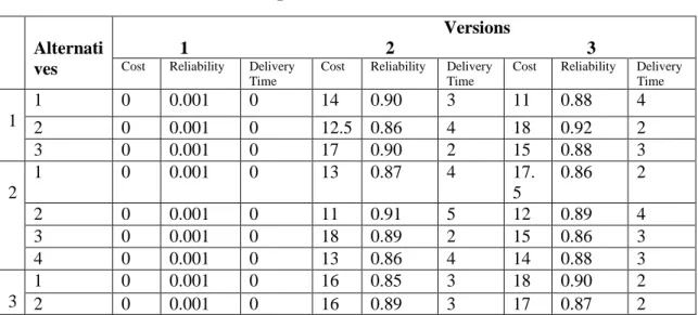
Consider a software system having two modules with more than one alternative for each module. The data sets for COTS and in-house developed components are given in Table-1 and table II, respectively. Let





 

 

1 2 3 1 2 3

3, 1, 2,3 , 1,3 , s 2 , 0.5, 0.3 and 0.2

L s  s   f  f  f  . It is also assumed

that t1.01,t2 .05andt3 .01

FUNCTIONS

VERSION

MODULE MODULE MODULE

Figure 1Structure of the software

1

f f2 fl

1

m

2

m

n

m

102

Table 1: Data set for COTS components

Table 2Data set for In-House conponents

4.1 Optimization Model – I

Table 3 presents the solution for optimization model I. The problem is solved using software package LINGO (Thiriez, [11]). The solution to the model gives the optimal component selection for the software system along with the corresponding cost and reliability of the overall system. The sensitivity analysis to the delivery time constraint has been performed. It is clearly seen from the table

Alternati ves

Versions

1 2 3 Cost Reliability Delivery

Time

Cost Reliability Delivery Time

Cost Reliability Delivery Time

1

1 0 0.001 0 14 0.90 3 11 0.88 4

2 0 0.001 0 12.5 0.86 4 18 0.92 2

3 0 0.001 0 17 0.90 2 15 0.88 3

2

1 0 0.001 0 13 0.87 4 17.

5

0.86 2

2 0 0.001 0 11 0.91 5 12 0.89 4

3 0 0.001 0 18 0.89 2 15 0.86 3

4 0 0.001 0 13 0.86 4 14 0.88 3

3

1 0 0.001 0 16 0.85 3 18 0.90 2

2 0 0.001 0 16 0.89 3 17 0.87 2

Module i Alternatives t_ij ij cij ij

1

1 8 0.005 5 0.002

2 6 0.005 4 0.002

3 7 0.005 4 0.002

2

1 9 0.005 5 0.002

2 5 0.005 2 0.002

3 6 0.005 4 0.002

4 5 0.005 3 0.002

3 1 6 0.005 4 0.002

103

that when the delivery time was 10 units, then only COTS components were selected. When the delivery time increases along with the COTS components, in house build components were also selected. When the delivery time was 12 units, only one in-house component was developed with the minimum cost 79 units attained at reliability level 0.85.Our system cost decreases while the corresponding reliability increases because the components developed in-house decreases the cost initially but later if the level of reliability has to be kept at 0.90 then by increasing delivery time by 5 and 9 units respectively, more in-house build components were selected which in turn increases the cost and reliability of the overall system. Redundancy is also there in all the four cases.

Table 3: Solution of Optimization Model I

4.2 Optimization Model-II

To illustrate optimization model for compatibility, we use previous results.

Case 1. Delivery Time is assumed to be 10 units.

We assume third alternative of second module is compatible with second and third alternatives of first module.

111 123 133 1

x x x 

Case No.

Delivery Time

COTS IN-House System Reliability

Overall system Cost

Joint Objective

Value

1 10 111 123 132

211 221 232 242 311 322

1 1 1

x x x

x x x x

x x

  

   

 

Nil 0.84 82 0.66

2 12 111 123 132

211 232 241 311 322

1 1 1

x x x

x x x

x x

  

  

 

22 1

y  0.85 79 0.68

3 17 111 123 132

211 221 232 311

1 1 1

x x x

x x x

x

  

  



24 32 1

y y  0.93 86 0.74

4 21 111 132

211 221 232 311

1 1 1

x x

x x x

x

 

  



12 24 32 1

104

211 221 232 242 1

x x x x 

311 322 1

x x 

It is observed that due to the compatibility condition, third alternative of first module is chosen as it is compatible with third alternative of second module. The system reliability for the above solution is 0.84 and cost is 81 units.

Case 2. Delivery Time is assumed to be 12 units.

We assume second alternative of third module is compatible with second and third alternatives of first module.

22 1

y 

;

111 123 133

211 232 241

311 322

1 1 1

x x x

x x x

x x

  

  

 

It is observed that due to the compatibility condition, third alternative of first module is chosen as it is compatible with second alternative of third module. The system reliability for the above solution is 0.85 and cost is 77 units.

Case 3. Delivery Time is assumed to be 10 units.

We assume third alternative of second module is compatible with second and third alternatives of first module.

24 32 1

y y 

111 123 133

211 221 232

311

1 1 1

x x x

x x x

x

  

  



It is observed that due to the compatibility condition, third alternative of first module is chosen as it is compatible with third alternative of second module. The system reliability for the above solution is 0.94 and cost is 84 units.

5. Conclusions

105

were also selected and different impacts on cost and reliability were considered. Redundancy was also there in all the cases.

References

[1] F. Belli and P. Jadrzejowicz, An approach to reliability optimization software with redundancy, IEEE Transaction of Soft. Engineering, vol.17/3(1991), pp. 310-312.

[2] O. Berman and U. D.Kumar, Optimization models for reliability of modular software system, IEEE Transactions of Software Engineering, vol. 19/11(1993), pp.1119-1123.

[3] A. Bertolino, and L. Strigini, On the use of testability measures for dependability assessment, IEEE Transactions on Software Engineering,

22/2(1996), pp.97-108.

[4] V. Cortellessa, F. Marinelli, and P. Potena, An optimization framework for “build-or-buy” decisions in software architecture, Computers and

Operations Research, vol.35(2008), pp. 3090-3106.

[5] L. M. Cysneiros and J.C.S. Leite, Nonfunctional requirements: from elicitation to conceptual models, IEEE transactions on Software

engineering, vol.30 (2004), pp. 328-350.

[6] A. M. Geoffrion, Proper efficiency and theory of vector maximization,

Journal of Mathematical Analysis and Application, vol.22 (1968), pp.

613-630.

[7] H. W.Jung and B. Choi, Optimization models for quality and cost of modular software system, European Journal of Operations Research,

vol.112(1998), pp. 613-619.

[8] P. K. Kapur, A.K. Bardhan and P.C. Jha, Optimal reliability allocation problem for a modular software system, OPSEARCH, vol.40/2(2003). [9] U. D. Kumar, Reliability analysis of fault tolerant recovery block,

OPSEARCH, vol.35(1998),pp. 281-294.

[10] R. E. Steuer, Multiple Criteria optimization: theory, computation and application, Wiley, New York ,1986.

[11] H. Thiriez, OR software LINGO, European Journal of Operational