umi-unc-3111.pdf

(1)

An Investigation of Cosolvent Flushing for the

Remediation of PAH’s from Former Manufactured Gas

Plant Sites

Arne P. Newman

A thesis submitted to the faculty of the University of North Carolina at Chapel Hill in partial fulfillment of the requirements for the degree of Master of Science in the Department of Environmental Science and Engineering, School of Public Health

Chapel Hill 2008

Approved by:

Advisor: Dr. Cass T. Miller

Reader: Dr. Gregory W. Characklis

(2)

Abstract

Arne Newman: An Investigation of Cosolvent Flushing for the Remediation of PAH’s from Former Manufactured Gas Plant Sites

Manufactured gas plant (MGP) operations across the United States during the late 19th and early 20th centuries resulted in the release of polycyclic aromatic hydrocarbons (PAH’s) into soil and groundwater systems, leading to degradation of groundwater quality and creating public health risks. Former MGP sites require appropriate cleanup methods; this study uses PAH-contaminated field soil to examine the potential for cosolvent flushing as an efficient remediation technology. Batch experiments examined the desorption and solubilization of PAH’s with cosolvent solutions; a log-linear

(3)

List of Tables

(7)

List of Figures

Figure 1 BT1 total PAH RP as a factor of fc... 34

Figure 2 BT2 RP as a factor of fc (24 and 48 hr samples)... 35

Figure 3 BT2 RP of individual PAH’s as a factor of fc (48 hr samples) ... 36

Figure 4 BT2 values for αβσ (24 and 48 hr samples)... 40

Figure 5 αβσ from batch experiments as a factor of literature log Kow values ... 41

Figure 6 PAH RP with an fc of 0.9 fc as a factor of equilibration time ... 41

Figure 7 Effluent concentration profile of 3H20 step tracer ... 43

Figure 8 SC1 and SC2 total PAH effluent concentrations and RP as a factor of relative flushing volume ... 45

Figure 9 SC1 and SC2 total PAH effluent concentration and RP as a factor of flushing time ... 46

Figure 10. Effluent concentrations of small columns (SC1 on left, SC2 on right); PHE, PYR, and BGP on secondary vertical axes... 47

Figure 11 Residual concentrations of individual PAH’s in SC1 and SC2... 48

Figure 12 SC2 residual total PAH concentrations by segment ... 48

Figure 13 Effluent concentration profile of 3H20 pulse as a factor of relative flushing volume... 49

Figure 14 Total PAH effluent concentrations and total mass removed as a factor of relative flushing volume ... 52

Figure 15 Large column effluent concentrations; PHE, BGP on secondary vertical axes (right side)... 53

(8)

(9)

List of Abbreviations and Symbols

1N One normal

3

H20 Tritiated water

α Cosolvent-sorbent interaction parameter

ACN Acetonitrile

ACE Acenapthene

ACY Acenapthylene

ad-10 Anthracene d-10

BAA Benzo[a]anthracene

BAP Benzo[a]pyrene

BBF Benzo[b]fluoranthene

β Water-cosolvent interaction parameter

BKF Benzo[k]fluoranthene

BGP Benzo[g,h,i]perylene

BT1 Batch test: fc range 0 to 1 BT2 Batch test: fc range .7 to 1 0

C Degrees Celsius

CaCl22H20 Calcium chloride dihydrate

CE Concentration extracted (mg/kg)

CI Initial concentration (mg/kg)

(10)

cm Centimeter

CHR Chrysene

D Dispersion coefficient (cm2/hr) D/uL Dimensionless dispersion coefficient

DBA Dibenzo[a,h]anthracene

DCM Methylene chloride

DI Deionized

DNAPL Dense non-aqueous phase liquid

Eq. Equation

fad Fraction ad-10 recovered

FLT Fluoranthene

FLU Fluorene

g gram

H2SO4 Hydrogen sulfate

HOC Hydrophobic organic compound

hr Hours

KCl Potassium chloride

kg Kilogram

Kp,m Equilibrium partitioning coefficient in mixed cosolvent (L/kg) Kp,w Aqueous equilibrium partitioning coefficient

KOW Octanol-water partitioning coefficient

L Column bed length

(11)

LC Large column

log Logarithm, base 10

LNAPL Light non-aqueous phase liquid

m Meter

mg Milligram

mL Milliliter

MI Initial mass (mg)

min Minute

Mm Mass in mixed cosolvent phase (mg)

MGP Manufactured gas plant

MgSO47H20 Magnesium sulfate

MRT Mean residence time

MW Molecular weight

Na2SO4 Sodium sulfate, anhydrous

NAP Naphthalene

NAPL Non-aqueous phase liquid NPL National Priority List O&M Operation and maintenance

OM Organic matter

PTFE Polytetrafluoroethylene

PV Pore volume

fc Cosolvent fraction

(12)

NaHCO3 Sodium bicarbonate

PAH Polycyclic aromatic hydrocarbon

PAT Pump-and-treat

PCE Perchloroethylene

PHE Phenanthrene

PPM Parts per million (mg/kg) PTFE Polytetrafluoroethylene

PYR Pyrene

R2 Regression correlation coefficient Rm Retardation factor in mixed cosolvent Rw Retardation factor in aqueous solution

RP Removal percentage (mg/mg)

RPD Relative percent difference

SC1 Small column experiment with an fc of 0.9 SC2 Small column experiment with an fc of 0.95

σ Cosolvency power

Sm Solubility in mixed cosolvent

Sw Aqueous solubility

u Pore velocity

(13)

(14)

1 Introduction

1.1 Groundwater

Groundwater is a vital source of fresh water, accounting for approximately 30% of the total global reserves and up to 98% when water tied up in glaciers and the polar ice caps is discounted (Foster and Chilton, 2003). It is estimated that 50% of global potable water supplies come from groundwater, and it is often a much more economical source than surface water. In the US, groundwater is used by 53% of citizens and accounts for approximately 20% of total water usage (Foster, 2006). While groundwater usage by humans dates back to early civilization, heavy exploitation did not begin until the 1950’s with major advances in both scientific knowledge and extraction technology. This newfound ability to extract groundwater on a large scale, combined with aquifer degradation and contamination, has led to a stress on groundwater resources at the national and global levels and an increased focus on groundwater quality issues.

The National Groundwater Association estimates that approximately 3% of

(15)

Council, 2004). Each of these contaminant classes can come from a variety of sources, resulting in degradation of water quality to varying degrees and requiring appropriate cleanup efforts (Hardesty and Ozdemiroglu, 2005).

1.2 Research Objective

One particularly prevalent source of groundwater contamination is former manufactured gas plant (MGP) sites, which release PAH’s into soil and groundwater systems. Several PAH’s are classified as carcinogenic, posing a threat to public health; they are recalcitrant compounds that may persist in the subsurface for centuries

(Khodadoust et al., 2000). Convential cleanup methods for MGP sites have proven inadequate in achieving remediation goals within a desirable time frame.

(16)

2 Background

2.1 Manufactured Gas Plant Sites

Manufactured gas was the nation’s primary energy source during the late 18th and early 19th century, relying on a variety of processes to produce gas from various

feedstocks. The estimate of total MGP’s in operation in the US over time varies greatly by source, in part due to differences in the definition of an MGP site. Brown’s Directory of American Gas Companies identified approximately 1,500 MGP sites operating

between 1890 and 1950, but the study was limited due to voluntary reporting (Murphy et al., 2005). An EPA report in 2004 found that from 1800 to the mid 1900s approximately 36,000-55,000 MGP’s were in operation in the US, and approximately 88% of these sites were suspected to have released contaminants (US EPA, 2004).

During the gas manufacturing process various byproducts were created, some reusable and others purely waste. Non-reusable residuals such as coal tar, iron filings, or contaminated wood chips were often disposed of on site or at nearby locations without an appropriate containment method. The size of these disposal sites ranges from less than an acre to approximately 200 acres, and they were often located near waterways or

(17)

by PAH’s (Murphy et al., 2005). Tars are dense, non-aqueous phase liquids (DNAPLs) that contain significant concentrations of PAH’s and are very difficult to remediate (Khodadoust et al., 2000). The high densities of DNAPLs often cause them to sink below the water table and collect in pools at impermeable layers where they are less accessible to cleanup actions. In other cases, in part due to high NAPL-water interfacial tensions, NAPLs may become entrapped within pore spaces by capillary forces and become resistant to mobilization (National Research Council, 2005). Contaminants tend to dissolve from the NAPL phase into bulk groundwater very slowly because of low

aqueous solubilities; therefore, NAPLs generally persist in soil and groundwater for long time scales; the expected life span of a subsurface NAPL ranges from several decades to a few centuries depending on specific contaminants and local flow characteristics (CH2MHill, 1997).

Overall, it is estimated that over 11 billion gallons of by-product tars were released into the environment, impacting thousands of acres and millions of gallons of water. Cleanup costs at a single site have ranged from a few thousand dollars to over $86 million, with a cost range at a “typical” site from $3-10 million. Depending on the extent of contamination at sites not yet investigated, this could lead to a total cleanup cost for MGP sites of $26-128 billion (US EPA, 2004).

2.2 Polycyclic Aromatic Hydrocarbons

(18)

organic materials, and occur as complex mixtures in ambient settings (Agency for Toxic Substances and Disease Registry, 1995). They range in molecular weight from 128 to 366 grams per mole, vary in structure from two to over six rings, and generally exist as

colorless solids in pure chemical form. The majority of PAH’s come from synthetic sources; the largest single source is wood burning in homes, followed by automobile and truck emissions. High concentrations of PAH’s can be found at hazardous waste sites such as wood-treatment plants and MGP’s; they are very common soil and groundwater pollutants (Agency for Toxic Substances and Disease Registry, 1995). In groundwater systems they are often found sorbed to soils or as part of a NAPL such as coal tar; they display extremely low solubilities in water, causing them to be very recalcitrant in the subsurface.

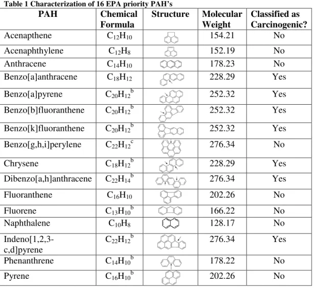
The EPA regulates 16 “priority” PAH’s (Table 1) representing the most prevalent, potentially harmful compounds found in the environment; benzo(a)pyrene is regarded as the most toxic and is often used as a benchmark contaminant. While no federal

(19)

former NPL sites. PAH’s were reported at over 600 of these sites, and this may even be an underestimate as it is unknown how many NPL sites were not evaluated for their presence (US EPA, 2007). It is notable that the 7 PAH’s classified as carcinogenic by ATSDR have the highest MWs (all at least 228.29 g/mol); therefore, high MW PAH’s are of particular importance in remedial considerations.

Table 1 Characterization of 16 EPA priority PAH’s

PAH Chemical

Formula

Structure Molecular

Weight

Classified as Carcinogenic?

Acenapthene C12H10 154.21 No

Acenaphthylene C12H8 152.19 No

Anthracene C14H10 178.23 No

Benzo[a]anthracene C18H12 228.29 Yes

Benzo[a]pyrene C20H12b 252.32 Yes

Benzo[b]fluoranthene C20H12b 252.32 Yes

Benzo[k]fluoranthene C20H12b 252.32 Yes

Benzo[g,h,i]perylene C22H12c 276.34 No

Chrysene C18H12b 228.29 Yes

Dibenzo[a,h]anthracene C22H14b 276.34 Yes

Fluoranthene C16H10 202.26 No

Fluorene C13H10b 166.22 No

Naphthalene C10H8 128.17 No

Indeno[1,2,3-c,d]pyrene

C22H12b 276.34 Yes

Phenanthrene C14H10b 178.22 No

Pyrene C16H10b 202.26 No

2.3 PAH Remediation at MGP Sites

(20)

oxidation, air sparging, thermal treatment, and pump-and-treat (PAT) (US EPA, 2004). PAT is the most prevalent groundwater remedy used at Superfund sites, but due to a number of shortcomings the overall effectiveness and the efficiency of this strategy with respect to time and cost has historically been very low. In order for PAT methods to remain a viable option for site cleanup in the future, particularly at PAH-contaminated MGP sites, significant improvements must be made in the ability to remove contaminants in an efficient manner.

2.4 Pump-and-Treat

Pump-and-treat is the most common remediation method for contaminated

groundwater systems, used either as a stand-alone treatment method or in combination with other methods at over 75% of NPL sites through 2007 (US EPA, 2007). The basis for PAT technology is the extraction of contaminated water from the subsurface and subsequent above-ground treatment. In a conventional PAT system, a set of underground injection wells pumps clean water into the soil and through the contaminated region, mobilizing the contaminated fluid toward a set of extraction wells (National Research Council, 1994). Once the contaminated water is removed through the extraction wells it is treated by one or more methods including adsorption, volatilization, precipitation, oxidation-reduction, or biotransformation (Bhandari et al., 2007). After treatment the water may be discharged to a local surface water body or in many cases reinjected

underground; reinjecting treated water as a form of recycling the flushing solution source can improve process efficiency.

(21)

dissolution of contaminants into the pumped solution, therefore contaminants that display low solubilities in water or preferentially sorb to soils present problems. NAPLs such as coal tar fall into this category; the inability to efficiently mobilize these contaminants towards extraction wells renders conventional PAT systems impractical because cleanup goals cannot be met in a reasonable time frame or at an acceptable cost (Kent and

Mosquera, 2001). The hydrogeologic setting also plays an important role in determining the feasibility of PAT methods. Groundwater systems with low hydraulic conductivities (below 10-5 cm/s is considered poor, greater than 10-3 cm/s is ideal) can prevent flushing at desired rates (Bhandari et al., 2007). Subsurface heterogeneities can lead to preferential flow patterns, missing portions of the contaminated zone and allowing for collection of contamination in areas of low permeability. Due to natural heterogeneities in all soil and groundwater systems, complete information regarding these hydrogeologic properties is impossible to achieve; estimates must be made using optimized sampling procedures and current modeling techniques. Studies of PAT systems are indicative of the importance of these chemical and physical limitations; an EPA study found that of 39 PAT systems underway in 2001, only 7 were estimated to have progressed to at least 80% of the restoration goal (EPA, 2001).

(22)

prohibitive due to the longevity of PAT systems; a study of 67 PAT actions found that 52% lasted from 0-5 years, 42% from 5-10 years, and 6% for 10-15 years (Congressional Budget Office, 1994). In order to minimize these costs it is important to reduce PAT remediation time by increasing the efficiency of contaminant removal.

2.5 Improving PAT Methods: Introduction and Physical

Processes

2.5.1 Decreasing PAT Time

In order to decrease the longevity of a PAT system, contaminants must be

removed through extraction wells at a faster rate. Higher pumping velocities require more energy and are therefore more expensive; in many cases faster pumping is physically impossible due to the hydrogeologic setting. For highly contaminated areas, especially those containing hydrophobic organic contaminants (HOC’s) such as PAH’s, it has been estimated that up to tens of thousands of PV of water may be required to remediate to regulatory levels (Augustijn et al., 1994). This impractical strategy can be avoided by increasing the mass transfer of contaminant into the flushing solution and improving the mobility of NAPLs, thereby increasing the concentration of contamination in extracted fluid and reducing the total flushing volume (Vf) required. Increased mass transfer can be created by affecting two physical processes: the dissolution of contaminants into the flushing solution and the desorption of contaminants into the bulk fluid phase.

(23)

Equilibrium dissolution from complex wastes is often described by Raoult’s law such that the concentration of component i (Ci) in contact with a complex solution (e.g. coal tar) can be determined by the simple relation

Ci = xiSi (Eq. 1)

where xiis the mole fraction of component i in the waste mixture and Si is the liquid

solubility of the ith component; this does not hold for non-ideal fluids (Augustijn et al., 1997). Dissolution has a linear relationship with the difference between aqueous solubility and solubility in the secondary phase (e.g. NAPL); therefore, solubility enhancements will increase mass transfer in a predictable manner.

Solubility is inversely related with the hydrophobicity of a compound; one index for determining hydrophobicity is the octanol-water partitioning coefficient of a

substance (Kow), measuring the ratio of concentrations of a compound in octanol and water in a mixture of the two liquids. Hydrophobicity is positively correlated with MW such that PAH’s of lower MW will solubilize into an aqueous solution more readily than the higher MW compounds. This effect makes high MW PAH’s of particular concern for PAT methods; even in cases where the flushing solution is adequate for the removal of two and three ring PAH’s, four, five and six ring PAH’s may remain in the NAPL or solid phase.

2.5.3 Desorption

In order to design an effective enhanced soil flushing technology for PAH

(24)

2007). Sorption includes two different processes, adsorption and absorption: adsorption is the attachment of contaminant to surfaces or interfaces, while absorption refers to the complete mixing of contaminant throughout the sorbent phase. PAH’s can generally be absorbed into soils in two ways: entrapment in soil micropores and structures (also called intraparticle diffusion) and absorption into soil organic matter (OM) (Shore et al., 2003).

PAH desorption from soils occurs in two stages according to how the contaminant is sorbed to the soil. The first stage, known as the instant or fast stage, entails the

relatively immediate release of contaminants either sorbed to the surface of or readily available within soil particles when exposed to a solvent, predominantly due to solubility increases. The second stage, known as the slow stage or nonequilibrium sorption, refers to the rate-limited process of PAH’s diffusing through the OM and/or microporous structures of the soil. It has been hypothesized that in many soils, especially those with high OM content, PAH diffusion through OM is the dominant slow stage process (Shore et al., 2003). OM has been described as a three-dimensional polymeric structure

perforated with voids, existing in a rigid, condensed state when in contact with an aqueous solution such as groundwater (Nkedi-kizza et al., 1989). Both the concentration and type of OM in soils affect this diffusive process; soils with high organic

concentrations may experience greater nonequilibrium sorption . Since the fast desorption stage is relatively instantaneous, speeding up desorption during the flushing process may be best achieved by affecting the properties of the soil OM.

2.5.4 Mobilization

(25)

tension, capillary forces holding the NAPL in place can be overtaken by pumping forces and moved toward extraction wells. Density-driven, gravitational and viscous forces may also come into play with reduced interfacial tensions, causing vertical mobilization of NAPLs. This is typically desirable with LNAPLs, as they float to the top of the water table and are more easily removed. In the case of DNAPLs such as coal tar, it may cause further contaminant migration towards an impermeable layer; this has been historically deemed problematic and hydraulic control of contaminants must be considered in remedial design (Augustijn et al. 1994). A recent technology designed to capture vertically mobilized DNAPLs, known as the Brine Barrier Remediation Technology (BBRT), may be a solution to this scenario. In this technology, a layer of dense brine is emplaced by injection above the impermeable layer; any vertically displaced DNAPLs will pool on top of the brine due to density differences and may be removed at that point (Hill et al., 2001).

2.6 Enhanced Soil Flushing

Injecting a flushing solution into the subsurface containing chemical additives can significantly improve the overall effectiveness, cost and time efficiency of PAT systems. This is achieved by increasing the mass transfer of contaminants into the fluid phase through enhanced solubilization and desorption of HOC’s created by the chemical additives. This method can be referred to as enhanced soil flushing; one well-studied form of enhanced soil flushing is solvent flushing.

2.6.1 Solvent Flushing

(26)

Enhanced soil flushing utilizing water-miscible organic solvents as chemical additives is typically referred to as in-situ solvent washing or solvent flushing; since the solvents are generally mixed with water they are often called cosolvents. The theoretical basis for this method is the well studied enhancement of solubility and desorption of HOC’s in aqueous solutions by cosolvents. Low-molecular-weight alcohols such as ethanol and methanol are the most common solvents of choice for in situ treatment methods; they are fully miscible in water, relatively biodegradable in the environment, and can increase the solubility of HOC’s by several orders of magnitude (Augustijn et al., 1994).

Physical Description

Adding an organic solvent to water decreases the polarity of the solvent mixture, increasing the solubility of nonpolar organic compounds (Augustijn et al., 1997). It is well established that the solubility of nonpolar contaminants such as PAH’s increases in a log-linear manner with increasing cosolvent volume fraction (fc) such that

log Sm = log Sw +βσfc (Eq. 2)

(27)

Solubility and sorption of HOC’s are inversely related; therefore, fast stage PAH desorption is expected to increase in a log-linear manner with the addition of cosolvent. The equilibrium partitioning constant Kp (L/kg), representing the ratio of the

concentration of sorbed contaminant (mg/kg) over the concentration of contaminant in solution (mg/L), has a relationship with fc such that

log Kp,m = log Kp,w – αβσfc (Eq. 3)

where Kp,m and Kp,w are the equilibrium partitioning constant for the mixed cosolvent and aqueous phases, respectively (Brussea et al., 1991). The parameter α is an empirical constant representing the deviation of the Kp-fc relationship from solubility dependence; a practical description for α is a quantification of the soil-cosolvent interactions. Cosolvent-sorbent interactions may cause positive (α>1) or negative deviations (α<1), depending on the system studied. The parameter σ is known as cosolvency power, a hypothetical partitioning coefficient for HOC’s between a cosolvent and water expressed as

σ = log(Sc/Sw) (Eq. 4)

where Sc and Sw represent the solubilities of the HOC in pure cosolvent and water, respectively (Rao et al., 1990). Cosolvency power has been described as the most important parameter in cosolvency theory as it quantitatively describes the relationship between a solute, cosolvent, and aqueous phase that drives increased solubilization (Augustijn et al., 1994).

Equilibrium sorption in transport problems is often evaluated in terms of a retardation factor (R) that represents the residence time of a contaminant in PV. R has a log-linear relationship with fc derived from Eq. 3 such that

(28)

where Rm and Rw represent the retardation factor in the mixed cosolvent and aqueous solutions, respectively (Nkedi-Rizza et al., 1987). Thus, contaminants should elute more efficiently with respect to relative Vf with increasing fc in column experiments and field applications.

A principal effect of cosolvent on soils is through interaction with soil OM; as the aqueous phase is mixed or replaced with a solvent the reduction in polarity causes the rigid, condensed polymeric structure of the OM to expand or “swell” and become more flexible. This process has been called the cosolvent effect and allows for the release of previously entrapped contaminants. Cosolvent effects are reversible; OM will recondense when the mixed cosolvent is replaced with an aqueous phase. Octanol is an organic solvent that is used as a surrogate for OM in partitioning behavior; therefore, the hydrophobicity index Kow can aid in the understanding of HOC sorption to soils

containing OM. Cosolvency power has been shown to correlate positively with Kow such that

σ = A log Kow + B (Eq. 6)

where both A and B are empirical constants applying to a specific compound (Chen and Delfino, 1997). This relationship signifies that cosolvent effects are greater on solutes that more readily partition into OM in aqueous solutions such as higher MW, more hydrophobic PAH’s.

(29)

cosolvents on OM is a significant benefit of solvent flushing, especially in soils with high OM concentrations capable of entrapping a significant percentage of resident PAH’s.

Field Precedent

Several field tests of alcohol flushing have found relative success in groundwater remediation of DNAPLs using alcohol flushing solutions; two examples focused on removal of perchloroethylene (PCE). The first study flushed two PV of a 95% ethanol, 5% water mixture over three days with approximate removal of 62-65% of initial PCE contamination (Jawitz et al., 2000). A second study performed in an isolated cell utilized a solution of approximately 70% ethanol and 30% water for approximately 10 PV over a 40-day period, removing an estimated 64% of PCE (Brooks et al., 2004). This study was able to successfully recycle flushing solution, with recycling accounting for over 50% of the total fluid injected; this allows for major cost reductions and is promising for future field applications.

(30)

monitoring and adaptive management of pumping rates and locations have the potential to significantly improve removal rates.

Cosolvent Choice

Methanol and ethanol are the two primary candidates for solvent flushing application and display very similar partitioning coefficients for PAH’s; therefore, it is very likely that their effectiveness in solubilizing and desorbing PAH’s is similar (Augustijn et al., 1994). An ex-situ solvent washing process using ethanol was tested on PAH-contaminated soil from a former MGP site and found total PAH removal of greater than 93% compared to Soxhlet extraction including a calculated 100.1% removal for the two-ring and three-ring compounds. A set of small column experiments testing the cosolvent effects of ethanol and methanol on MGP field soil contaminated with PAHs found comparable removal rates for the two alcohols at a flushing solution volume fraction of 0.85 (Chen et al., 2005).

Methanol has received greater attention in the literature with respect to HOC desorption parameters, allowing for more direct comparison with experimental findings. A set of batch and column experiments found that methanol-water-soil systems spiked with PAH’s displayed strong solubility and desorption enhancements and supported the hypothesis that nonequilibrium sorption is dependent on diffusion through OM

(31)

(32)

3 Materials and Methods

3.1 Materials

3.1.1 Soil Properties

The soil used in all experiments comes from a one-hectare former MGP site in Salisbury, NC. Samples were taken at a depth of approximately 1.2 m; soil was placed in plastic bags which were stored in 7 sealed buckets. The buckets were kept in a 4 0C walk-in refrigerator for the duration of this research to minimize PAH losses due to volatilization.

Analysis performed by Stephen Richardson determined that pure soil hydraulic conductivities were too low for column experiments; through experimentation it was determined that a 1:1 (g/g) mixture of field soil and 40/50 grain Accusand would provide the needed increase in conductivity. This mixture was used in several batch experiments and all column experiments. To create this blend, the field soil and Accusand were mixed together using a mortar and pestle. Properties of the soil/sand mix as found by the lab group of Dr. Aitken are listed in Table 2.

Table 2 Properties of soil/sand mix

Sand content 82.9%

Silt content 13.8%

Clay content 3.3%

Soil pH 7.6±0.1

Inorganic carbon 7.0±1.6 %

Organic matter 8.3±1.3%

Bulk density 2.6±0.1 g/cm3

(33)

Initial analysis of the pure Salisbury soil found an average total PAH

concentration of 863 PPM with a relative percent difference (RPD) of 18.84%, consistent with the findings of Dr. Aitken’s group; soil PAH concentrations varied widely over experiments due to natural heterogeneity in field concentrations. No free phase coal tar was observed; the bulk of PAH mass existed sorbed to the soil. This is an important consideration for remediation as it indicates that mobilization through reduced interfacial tension would be negligible, causing solubilization and desorption of PAH’s to be the primary processes of concern.

It is important to note that the soil OM content is high at 8.3±1.3%; it is likely that nonequilibrium sorption processes will exist and be dominated by diffusion through OM. Sorption kinetics of PAHs in the field soil are likely affected by aging as found in

previous studies, making it more difficult to predict the desorbable fraction of contaminant and rate of release (Shor and Rockne 2003). It is important to test aged, contaminated soils in order to better reflect the processes that would occur at field sites; freshly spiked soils may behave in a more ideal manner, less applicable to field-scale implementation.

3.1.2 Soil Preparation

(34)

(mL:g) water to soil mixture. The mixture was stirred for a 30-minute period; samples of the soil mixture were taken using volumetric pipettes and added to pre-weighed

centrifuge vials. The vials were centrifuged and resulting supernatant poured off, leaving a layer of wet soil. Several vials were set aside for soil moisture content analysis,

performed by fully drying the soil at approximately 100 0C overnight and determining the weight difference between wet and dry soil. The weight of wet soil in sample vials was then adjusted for moisture content (approximately 20% across experiments); all soil weights reported in this document are by dry weight.

The slurry method was not feasible for batch experiments using the soil/sand mixture due to separation of Accusand and field soil during stirring with water. Instead, the soil/sand mix was added directly to vials and a soil moisture content analysis

performed; moisture content of the mixture was approximately 7% across experiments.

3.2 Analytical Methods

All PAH samples were analyzed by HPLC equipped with Waters 2475 Multi-Wavelength programmable fluorescence detector for quantification. A 10-cm LC-PAH column (Supelco 59134) was used with a mobile phase of an acetonitrile (ACN, Fisher Scientific A998-4) and water (Fisher Scientific W5-4) gradient . Flow and wavelength programs were modified from those used by Dr. Aitken’s laboratory group. Of the 16 EPA priority PAH’s, 14 were consistently quantifiable with good replication;

(35)

analysis of differences in behavior with variation of individual PAH characteristics, notably MW and hydrophobicity.

Calibration curves for the EPA priority compounds were performed using a 16 PAH standard solution (Supelco 4-8743). Calibration curves for anthracene d-10 (ad-10), an internal standard, were performed using solutions of solid phase ad-10 (Supelco 44-2456) in ACN.

3.3 Batch Experiment Methods

3.3.1 General Methods

Samples

Batch tests were designed to examine the ability of flushing solutions to desorb and solubilize PAH’s from the Salisbury field soil. In each experiment, known amounts of soil and solution were added to 35-mL glass centrifuge vials with

polytetrafluoroethylene (PTFE) septa screw caps along with several 5-mm glass beads to encourage mixing during equilibration. The vials were then sealed with Parafilm and allowed to equilibrate on a rotating tumbler for a set period of time. After the

(36)

097207). During filtration, the first 1.5 mL was sent to waste to minimize the effects of sorption onto filters.

Extracts

PAH’s were extracted from the remaining soil using a 2 round method developed by the lab group of Dr. Aitken. Before PAH extraction, a known amount of anthracene d-10 (ad-d-10) was added to each vial as an internal standard to control for sample loss, volatilization, instrument drift, or other sources sample error. The final PAH

concentrations of each vial were adjusted based on the fraction of ad-10 recovered (fad) during extraction such that

Cadjusted = Canalyzed / fad (Eq. 7)

Values of fad ranged from 0.65 to 1.13 over the course of experiments, with an average of 0.85±0.15.

(37)

Data Analysis

The initial total PAH mass in each vial was determined by a mass balance of PAH’s removed to the fluid (mixed cosolvent) phase (Mm) and the PAH’s extracted (Me) such that

MI = Mm + Me (Eq. 8)

Where MI represents the initial PAH mass in the vial soil. Concentrations were determined by dividing PAH mass by vial soil weight. Concentrations are reported as parts per million (PPM) by mass, calculated as mg PAH per kg of dry soil. With differing initial PAH concentrations in every vial due to inherent contaminant distribution

heterogeneity in the field soil, directly comparing concentrations of PAH’s in the

cosolvent phase does not provide a good metric for comparison between samples; instead several other metrics are used.

PAH removal percentage (RP) is used as a practical metric representing the fraction of total PAH’s removed from the soil into solution, determined by

RP = 100 x (Mm / MI) (Eq. 9)

RP was determined for each individual PAH; calculation of total PAH removal in the vial was performed by a summation of all individual PAH’s removed to the mixed cosolvent phase, divided by the sum of all individual (i) PAH’s remaining sorbed to the soil:

Total PAH RP = 100 x Σi Mim / Σ MiI (Eq. 10)

Equilibrium sorption partition coefficients Kp,m (L/mg) are an important metric, determined by the ratio of the residual sorbed PAH concentration (CE, mg/kg) to concentration of PAH’s in mixed cosolvent phase (Cm, mg/L) such that

(38)

A plot of log Kp,m versus fc was used to test the relationship expressed in Eq. 3. The product αβσ was determined for each PAH, representative of the combination of cosolvency power, soil-cosolvent, and cosolvent-water interactions responsible for the fluctuation of Kp,m with fc. This was calculated by predicting a hypothetical Kp,w value for each PAH based on the Kp,m vs. fc regression, and dividing the difference between log Kp,w and log Kp,m by fc. Calculations were only performed for the range of fc values that held to the fc/log Kp,m relationship; the average αβσ across all fcs is reported.

3.3.2 Experimental Design

BT1: Methanol Batch Test of fc Range 0 to 1

The first batch experiment studied methanol at fc of 0, 0.2, 0.4, 0.6, 0.8, and 1 to test the RP and desorption of the aged field soil in cosolvent. Approximately 1.5 grams of pure field soil and 20 mL of cosolvent solution were added to each centrifuge vial for an equilibration period of 48 hr.

BT2: Methanol Batch Test of fc Range 0.7 to 1

A second experiment was performed to examine RP and desorption kinetics of methanol in the soil/sand mixture at a fc range of 0.7 to 1 by intervals of 0.05,

(39)

tested at equilibration periods of 24 and 48 hr to look for rate-dependent desorption differences. Approximately 4 grams of the soil/sand mixture and 20 mL of cosolvent solution were added to the vials.

BT3: Methanol Rate Release Batch Test

PAH removal with a methanol fc of 0.9 was examined for the effects of rate limited desorption through a batch experiment with sample vials equilibrating for 1, 2, 4, 8, and 16, 24, 48, 72, and 96 hr. The extended time range was chosen to examine

desorption over multiple time scales (days and hr); a methanol fc of 0.9 was used to represent a viable field flushing solution based on methanol fc experimental data and field precedent for an fc of above 0.9 (Brooks et al., 2004; Jawitz et al., 2000). Approximately 4 grams of the soil/sand mixture and 20 mL of solution were added to each vial.

3.4 Small Column Experiment Methods

3.4.1 General Methods

Small column experiments were designed to study the ability of cosolvent solution to transport PAH’s with flow based on solubility and desorption enhancements. High fc values were chosen based on effectiveness in batch experiments, field precedent, and the goal of maximizing the effects of methanol cosolvency power.

(40)

connected to the insert and led to a PHD 440 programmable syringe pump. A wet packing procedure was used to minimize air entrapment during setup; columns were packed with the soil/sand mixture. De-aired water was pumped upward through the base of the column, and an initial 30/40 grain Accusand bed was poured into the water from the column top in order to retain soil fines that may have otherwise clogged the effluent port. After leveling the sand bed, soil was slowly dropped into the water from the top of the column, always maintaining a water level of at least at least 2 cm above the soil; the column was gently agitated every few minutes to ensure air pockets were removed during soil addition. After the desired amount of soil was added, the column top was sealed with parafilm and allowed to settle overnight. The following day a plastic insert with a

stainless steel end facing the soil was inserted downwards to fill extra space; this insert was also connected to the syringe pump by plastic tubing. The plastic tubing at the base of the column was disconnected from the pump, removed from the column base and replaced with stainless steel tubing to minimize effluent sorption. The column was allowed to equilibrate further with de-aired DI water pumped through slowly for 24 hr. Flushing solution was pumped from top to bottom, with effluent collected at the end of the stainless steel line; all column effluent was captured during experiments, enabling a PAH mass balance.

(41)

refrigerator to prevent volatilization or photodegradation of PAH’s, diluted to within optimal concentrations for HPLC analysis and filtered.

The post-flushing soil extraction procedure was the same as for the batch experiments, although different sampling methods for determining residual PAH distributions were used in each experiment.

3.4.2 Experimental Design

SC1:0.9 Methanol fc Flush

The column was packed with 159.75g of the sand/soil mix and a sand bed of 8.32 g at the base, with a total bed height of 20.5 cm.

A step tracer test was performed after the methanol flush for accurate

measurement of column properties using tritiated water (3H20), a non-reactive radioactive material. The column porosity, PV, mean residence time (MRT), and dispersion

parameters were determined from tracer results.

After an initial equilibration period, a methanol solution with an fc of 0.9 was flushed through the column at a pore velocity of 56.7 cm/day and flow rate of 5.334 mL/hr. Analysis of effluent PAH’s was performed during flushing; once a period of extended tailing was reached, at 6.22 PV, de-aired DI water was pumped through the column to displace resident methanol. Total flushing time was approximately 62.3 hr.

All of the column soil was extracted post-flushing and separated into 9 segments based on bed depth to study residual contaminant distribution; soil remaining on the column was rinsed off and analyzed to complete the mass balance..

(42)

The second column was packed with 172.19 g of soil/sand mix, with an Accusand bed at the base of 9.99 g, creating a total bed height of 22.2 cm. The column PV,

porosity, and MRT were estimated to be 50.1 mL, 0.463, and 24 hr; due to high accuracy of initial estimates (within 0.05%) of PV and porosity for SC1 and the time consuming nature of tracer tests, a tracer was not performed for SC2. After the initial equilibration period, a methanol solution with an fc of 0.95 was pumped through the column at a pore velocity of 22 cm/day and flow rate of 2.041 mL/hr. This flow rate was chosen in order to create a MRT of approximately 24 hr, allowing desorption more time to reach near-equilibrium than in SC1.

A total of 8.01 PV of methanol solution was pumped through, followed by 68 mL of de-aired DI water to displace the methanol. A flow interruption was performed at 5.46 PV; the pump was shut down and the column closed off for a 48 hr period. The purpose of this interruption was to test for rate-limited desorption; this has been done successfully in past studies (Brusseau et al., 1997). When desorption is rate-limited, effluent

concentrations will show a spike after the interruption; the size and shape of this spike can provide information about the magnitude of desorption nonequilibrium due to rate limitations.

The column was segmented into 4 soil sections and the sand bed for soil

(43)

3.5 Large-Scale Column Experiment Methods

The large column experiment was designed as a simplified, one-dimensional representation of solvent flushing for field application. The larger scale of the column allowed for improved simulation of inherent subsurface heterogeneities and variation in soil properties; sampling ports distributed over the length of the column enable study of contaminant spatial distribution. Efficient PAH removal from the large column may indicate the potential for success at the field scale.

The column was specially constructed by the UNC Environmental Science and Engineering shop; the body was made of stainless steel with a height of 110 cm and inner diameter of 10.2 cm; 3 soil sampling ports were built in at evenly spaced vertical

intervals. The top of the column was sealed by a removable cap equipped with a pressure gauge and inlet port; PTFE tubing connected the inlet port to a peristaltic pump (Eldex Laboratories PN 1005 A-60-8). A switch valve at the base attached to two effluent lines: one made of stainless steel, for use during sampling to prevent sorption of PAH’s to PTFE, and a second PTFE line for effluent sent to waste. Flushing solution was pumped from a sealed 20 L carboy. Discrete effluent samples were collected at set intervals in 40-mL glass vials, sealed with PTFE screw caps and pre-filled with 10 40-mL of ACN to decrease PAH volatilization and sorption to glass. Samples were stored in a closed box in a 4 0C refrigerator to prevent photodegradation and volatilization until prepared for HPLC analysis. Effluent flow rate and column pressure were measured at each sampling interval.

(44)

802 g bed of Accusand was added at the base of the colum with a thickness of

approximately 5 cm; there was a 5 cm aqueous layer between the top of the soil bed and the column top. After setup, the column was flushed with an aqueous solution designed to represent ambient groundwater; components of simulated groundwater were 1.83 g CaCl22H20, 1.01g MgSO47H20, 2.19g NaHCO3, 1 mL of 8.77 g/L KCl solution, and 1g of1N H2SO4 solution in 20 L DI water. The column experienced continuous flow with this mixture at a flow rate of 1.5 mL/min and pore velocity of 56.7 cm/day for a period of approximately 11 months before cosolvent flushing in order to equilibrate the system and test for mechanical issues (e.g. pump failure, leaks, etc.).

A pulse tracer test was performed with 3H20 before the cosolvent flush for accurate determination of the column porosity, PV and dispersion.

Cosolvent flushing was performed continuously using a methanol solution with an fc of 0.95 for 13.56 PV over a period of 13 days, 14 hr and 23 min at a flow rate of 2.4 mL/min and corresponding pore velocity of 99 cm/day.

Soil samples were taken from the 3 ports and the top of the soil bed before and after flushing and analyzed for PAH content using the same extraction procedure as the batch and small column experiments.

(45)

(46)

4 Results and Discussion

4.1 Batch Experiments

4.1.1 Varying Cosolvent Fractions

Total PAH Concentrations

The average total PAH content per vial in BT1 and BT2 were 579 ± 205 PPM (pure soil) and 546 ±439 PPM (sand/soil mix), respectively. Variation in contaminant concentration between vials in BT2 was driven by several samples with unusually high PAH levels; removing these outliers results in an average total PAH concentration of 430±68 PPM for BT2. Due to analytical error, NAP and FLU are not included in the BT1 total and ANT is not included in the BT2 total. Comparing only compounds analyzed in both experiments leads to average total PAH concentrations by difference (excluding outliers) of 553 and 378 PPM for BT1 and BT2, respectively. Noting that sand/soil mixtures should theoretically contain PAH concentrations ½ that of pure soil mixtures, the significant difference in average PPM is a reminder of the uneven distribution of PAH’s within the soil. While several vials contained highly concentrated pockets of PAH’s, a large difference in concentrations is still observed after the removal of outliers.

Removal Percentage

(47)

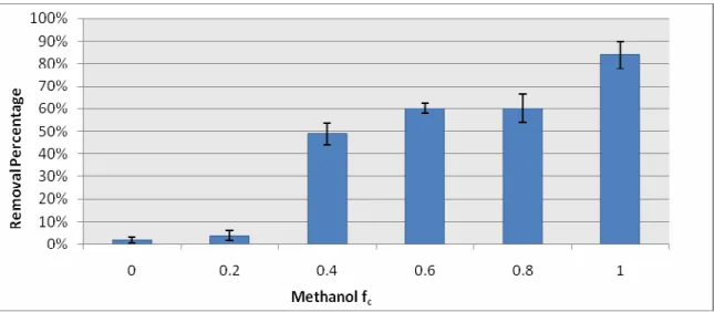
(Figure 1). Removal for an fc of 0.8 does not appear to fit the increasing trend, largely due to a single sample that recovered less than 10% of benzo[a]anthracene (BAA), which accounted for close to 1/3 of the total vial PAH mass; the reason for this low recovery is not clear. It is notable that BAA recovery was low across all values of fc.

Figure 1 BT1 total PAH RP as a factor of fc

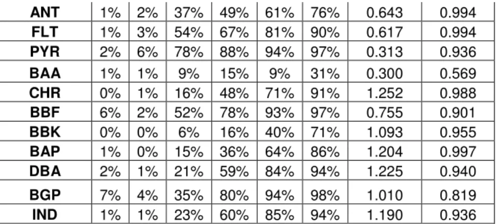
Observing removal of individual PAH’s in Table 3shows that while fc’s of 0.4 and 0.6 showed differentiation in average RP between low and high MW compounds, similar to a chromatographic effect, there was no distinct relationship between MW and RP for samples at an fc of 0.8 or 1. Linear regressions performed between RP and fc for individual PAH’s over a range of 0.4 to 1 show high R2 values. The linear relationship did not hold over the full fc range of 0 to 1, supporting previous findings that the fraction of HOCs that desorb quickly may not increase until a threshold cosolvent concentration in some soils (Brusseau et al., 1991).

Table 3: BT1 RP values as a factor of fc; regression statistics for fc vs. RP Compound RP Values with fc Regression

(48)

ANT 1% 2% 37% 49% 61% 76% 0.643 0.994

FLT 1% 3% 54% 67% 81% 90% 0.617 0.994

PYR 2% 6% 78% 88% 94% 97% 0.313 0.936

BAA 1% 1% 9% 15% 9% 31% 0.300 0.569

CHR 0% 1% 16% 48% 71% 91% 1.252 0.988

BBF 6% 2% 52% 78% 93% 97% 0.755 0.901

BBK 0% 0% 6% 16% 40% 71% 1.093 0.955

BAP 1% 0% 15% 36% 64% 86% 1.204 0.997

DBA 2% 1% 21% 59% 84% 94% 1.225 0.940

BGP 7% 4% 35% 80% 94% 98% 1.010 0.819

IND 1% 1% 23% 60% 85% 94% 1.190 0.936

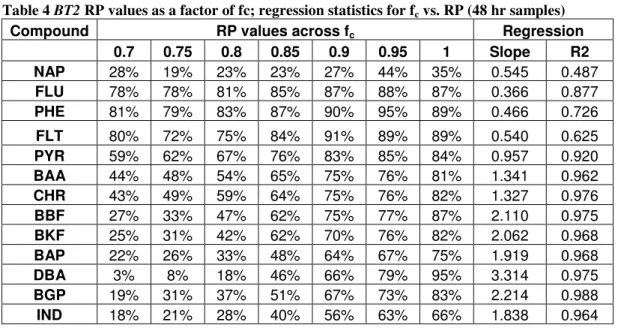
RP for PAH’s generally increased with fc from 0.7 to 1 in BT2, but linear

regressions returned relatively low R2 values, likely due to soil variation causing noise in the data; this was not as noticeable across the fc range 0 to1, potentially because the ratio of noise to change in RP was much lower over fc intervals of 0.2. The 48-hr samples averaged slightly higher (not statistically significant) RPs than the 24-hr samples at fc’s of 0.7, 0.75, 0.85, and 0.9; these differences were driven primarily by increased BGP removal for the 48 hr samples, suggesting that BGP removal experiences greater desorption rate effects than other PAH’s.

(49)

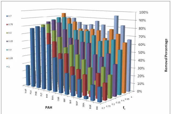
Increased removal between fcs of 0.7 and 1 appeared to be driven primarily by improved desorption and solubilization of the higher MW PAH’s. This is evident visually when looking at Figure 3, showing RP for individual PAH’s versus fc for the 48 hr

samples (24 hr data was comparable). While lower MW compounds displayed relatively minor removal improvements with fc increase from 0.7 to 1, the higher MW PAH’s showed much more drastic improvements (PAH’s in order of MW, increasing from left to right).

Figure 3 BT2 RP of individual PAH’s as a factor of fc (48 hr samples)

(50)

to coelute high and low MW PAH’s. Each of the seven PAH’s classified as carcinogenic show a correlation coefficient of greater than 0.96.

While total PAH removals were similar for both experiments at fc’s of 0.8 and 1, BT2 showed lower RPs for the middle and high MW compounds than BT1, especially at fc’s of 0.7 to 0.85. The low recoveries of BAA in BT1 balanced the generally lower RPs of the rest of the compounds in BT2 to create similar total PAH RPs. There are several possible explanations for the lower RPs in BT2; potentially the OM properties of BT2 soil were less amenable to the release of contaminants due to natural variability in the field soil. Another possibility is the difference in soil mass per vial between the experiments. The BT2 vials have greater solid material surface area; therefore, if similar Kp,m

coefficients were seen in the two experiments BT2 vials would have greater residual sorbed PAH concentrations. While PAH’s may not attach to the Accusand, the pure soil mass in BT2 vials is still greater than BT1 vials by an average of approximately 0.5 g.

Table 4 BT2 RP values as a factor of fc; regression statistics for fc vs. RP (48 hr samples)

Compound RP values across fc Regression

0.7 0.75 0.8 0.85 0.9 0.95 1 Slope R2

NAP 28% 19% 23% 23% 27% 44% 35% 0.545 0.487

FLU 78% 78% 81% 85% 87% 88% 87% 0.366 0.877

PHE 81% 79% 83% 87% 90% 95% 89% 0.466 0.726

FLT 80% 72% 75% 84% 91% 89% 89% 0.540 0.625

PYR 59% 62% 67% 76% 83% 85% 84% 0.957 0.920

BAA 44% 48% 54% 65% 75% 76% 81% 1.341 0.962

CHR 43% 49% 59% 64% 75% 76% 82% 1.327 0.976

BBF 27% 33% 47% 62% 75% 77% 87% 2.110 0.975

BKF 25% 31% 42% 62% 70% 76% 82% 2.062 0.968

BAP 22% 26% 33% 48% 64% 67% 75% 1.919 0.968

DBA 3% 8% 18% 46% 66% 79% 95% 3.314 0.975

BGP 19% 31% 37% 51% 67% 73% 83% 2.214 0.988

IND 18% 21% 28% 40% 56% 63% 66% 1.838 0.964

(51)

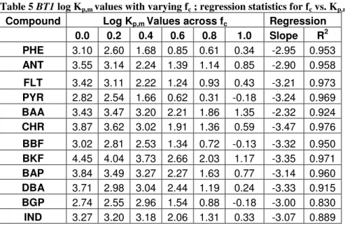
Kp,m values varied between the two experiments; log Kp,m showed a strong linear relationship with fc for most PAH’s between an fc of 0.04 and 1 in BT1. Yet in BT2, while fc values of 0.75 to 1 showed a linear relationship with log Kp,m; the 0.7 fc samples did not fit the regression. This may be consistent with previous literature findings that suggest some desorption relationships only hold up to an fc of 0.7 (Brussea et al., 1991; Augustijn et al., 1994); it may also be the result of experimental error or variation in soil properties.

Kp,m values at comparable fc (0.8 and 1) were generally lower for BT2, indicating that for most compounds PAH’s partitioned more readily into the cosolvent phase when in contact with the soil/sand mixture than pure soil. This is an intuitive observation because it is unlikely that a significant amount of PAHs sorbed to the OM-free sand while redistributing during the equilibration period; therefore, a large fraction of the solid surface area did not contain PAHs, decreasing CE of the mixture.

Table 5 BT1 log Kp,m values with varying fc ; regression statistics for fc vs. Kp,m Compound Log Kp,m Values across fc Regression

0.0 0.2 0.4 0.6 0.8 1.0 Slope R2

PHE 3.10 2.60 1.68 0.85 0.61 0.34 -2.95 0.953

ANT 3.55 3.14 2.24 1.39 1.14 0.85 -2.90 0.958

FLT 3.42 3.11 2.22 1.24 0.93 0.43 -3.21 0.973

PYR 2.82 2.54 1.66 0.62 0.31 -0.18 -3.24 0.969

BAA 3.43 3.47 3.20 2.21 1.86 1.35 -2.32 0.924

CHR 3.87 3.62 3.02 1.91 1.36 0.59 -3.47 0.976

BBF 3.02 2.81 2.53 1.34 0.72 -0.13 -3.32 0.950

BKF 4.45 4.04 3.73 2.66 2.03 1.17 -3.35 0.971

BAP 3.84 3.49 3.27 2.27 1.63 0.77 -3.14 0.960

DBA 3.71 2.98 3.04 2.44 1.19 0.24 -3.33 0.915

BGP 2.74 2.55 2.96 1.54 0.88 -0.18 -3.00 0.830

IND 3.27 3.20 3.18 2.06 1.31 0.33 -3.07 0.889

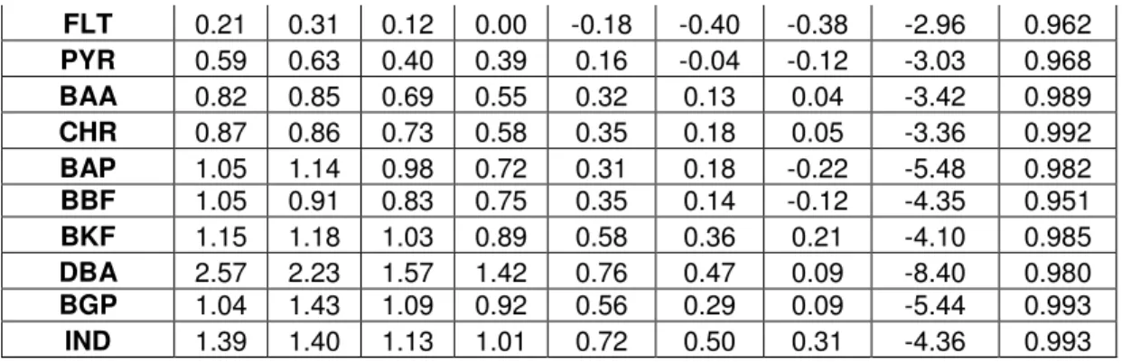
Table 6 BT2 log Kp,m values with varying fc ; regression statistics for fc vs. Kp,m (24 hr samples) Compound Log Kp,m values across fc Regression

0.7 0.75 0.8 0.85 0.9 0.95 1 Slope R2

NAP 1.75 1.47 1.16 1.22 1.28 0.83 0.88 -2.23 0.719

(52)

FLT 0.21 0.31 0.12 0.00 -0.18 -0.40 -0.38 -2.96 0.962

PYR 0.59 0.63 0.40 0.39 0.16 -0.04 -0.12 -3.03 0.968

BAA 0.82 0.85 0.69 0.55 0.32 0.13 0.04 -3.42 0.989

CHR 0.87 0.86 0.73 0.58 0.35 0.18 0.05 -3.36 0.992

BAP 1.05 1.14 0.98 0.72 0.31 0.18 -0.22 -5.48 0.982

BBF 1.05 0.91 0.83 0.75 0.35 0.14 -0.12 -4.35 0.951

BKF 1.15 1.18 1.03 0.89 0.58 0.36 0.21 -4.10 0.985

DBA 2.57 2.23 1.57 1.42 0.76 0.47 0.09 -8.40 0.980

BGP 1.04 1.43 1.09 0.92 0.56 0.29 0.09 -5.44 0.993

IND 1.39 1.40 1.13 1.01 0.72 0.50 0.31 -4.36 0.993

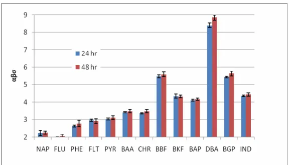
Values for αβσ were calculated for methanol over the range of fc from 0.4 to 1 for BT1 and 0.7 to 1 for BT2. Both sets of αβσ were lower than σ values presented in the literature for methanol-water-PAH systems, suggesting that αβ<1 for the aged field soil. An αβ value of less than one indicates that the cosolvent-sorbent and cosolvent-water interactions led to a decreased overall effectiveness of cosolvent to remove PAH’s to the fluid phase.

Table 7 Batch test αβσ values compared to literature σ values

Compound BT1 αβσ BT2 αβσ Literature σ

NAP - 2.23 3.72a

FLU - 1.98 4.12a

PHE 1.27 2.63 4.61a, 4.24b

ANT 1.22 - 4.67a, 4.06b

FLT 1.54 2.96 5.31a, 4.65b

PYR 1.70 3.03 5.19a, 4.69b

BAA - 3.42 5.74a, 5.22b

CHR 3.03 3.36 5.68a, 4.4b

BBF 2.58 5.48 6.44a, 6.53b

BKF 2.64 4.36 6.51a

BAP 2.59 4.10 5.95a, 4.05b

DBA 3.04 8.40 6.5a

BGP 3.27 5.44 6.9a

IND 2.94 4.36 6.66a

a - (Chen and Delfino, 1997), b - (Lane and Loehr, 1992)

Another possible explanation for this behavior is that sorption did not reach equilibrium during the 24 or 48 hr periods, and with a longer equilibration time αβσ

(53)

entrapment within OM. Using a common Kp,w value in calculations, 12 of 14 PAH’s in 48- hr samples did show marginally higher (only statistically significant for DBA and BGP) αβσ values than 24-hr samples.

Figure 4 BT2 values for αβσ (24 and 48 hr samples)

A linear trend between log Kow and αβσ was apparent for both experiments in regressions as suggested in Eq. 6 ; literature linear regression analysis performed on a range of cosolvents (Morris et al., 1988) found the slope of the coefficient A in

(54)

Figure 5 αβσ from batch experiments as a factor of literature log Kow coefficient

4.1.2 Methanol Rate Release Experiment

The average total PAH concentration per vial was 291 ±78 PPM. No relationship was evident between equilibration time and RP over the range of 1 to 96 hr; all time period averages were within a standard deviation (6%) of the total RP average at 81% (Figure 6).

(55)

A potential interpretation of this finding is that the swelling of OM caused by cosolvent is relatively immediate; at a high fc this results in a quick release and solubilization of entrapped contaminants. The data does not match the proposed two-stage process for sorption or behavior suggested by BT1 and BT2 results; further slow stage desorption was expected after the initial immediate release, and it is concerning that average RP did not show gradual movement toward 100%. While the results are a

promising indication that desorption equilibrium may be reached very quickly during flushing, they raise the possibility that a fraction of PAH’s may be inaccessible to

cosolvent. RP was consistent across samples, yet Kp,m values for individual PAH’s varied widely. Kp,m did display a rough trend of decreasing over time for several PAH’s based on individual vial data, indicating that greater partitioning was occurring into the cosolvent phase with longer equilibrations; regressions performed to quantitatively examine this trend returned very low correlation coefficients. The significant variation between individual samples caused averaged Kp,m values to show no trend over time visually or quantitatively.

(56)

4.2 Small Column Experiments

4.2.1 Tracer Results

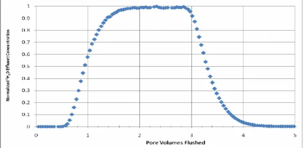
Calculations based on the results of the SC1 tracer test found a PV of 46.3 mL, a porosity of 0.463, and an MRT of 8 hr and 41 min. The dispersion coefficient D (cm2/hr) was 1.78. A dimensionless dispersion coefficient D/uL was determined to allow for comparison between SC1 and the large column; u represents the pore velocity and L the column length. The value of D/uL for SC1 was .037, very low for a field soil. The normalized 3H20 effluent concentration plot shows a relatively symmetrical profile, indicating low non-ideality conditions (Figure 7).

Figure 7 Effluent concentration profile of 3H20 step tracer

4.2.2 Initial Concentration and Total Removal

(57)

effluent, were 74.1g (SC1) and 87.6g (SC2), resulting in total PAH removal percentages over the duration of the flushing period at an estimated 78% and 89%.

4.2.3 Effluent Concentration and Total PAH Profiles

Effluent concentration profiles (Figure 8 and 9) showed behavior consistent with previous literature findings; the sharp increase in effluent PAH concentration at

approximately 1 PV is assumed to correspond with methanol breakthrough (Augustijn et al., 1994). Dashed lines on effluent concentration figures represent the period of flow interruption for SC2.

SC2 displayed an increased maximum effluent PAH concentration, a more compressed, symmetrical peak and reduced tailing compared to SC1; the primary driver for this behavior is the increase in Kp,m due to a higher fc in SC2. These results are in agreement with column tests of methanol solutions with varying fc’s flushed through soils spiked with PAH’s (Augustijn et al., 1994). The variation in MRT’s (8 hr and 41 min versus approximately 24 hr), allowing for longer equilibration of desorption in SC2 may have also played a role in creating these differences. The increased effluent

concentrations and reduced tailing allow for much more efficient PAH removal with respect to volume flushed. It is apparent that PAH’s favored desorption strongly enough in the 0.95 fc solution that the majority of sorbed mass was released quickly and

transported with flow.

The 48 hr flow interruption in SC2 resulted in an increase in effluent

(58)

Figure 8 SC1 and SC2 total PAH effluent concentrations and RP as a factor of relative flushing volume

(59)

Figure 9 SC1 and SC2 total PAH effluent concentration and RP as a factor of flushing time

4.2.4 Individual PAH Profiles

(60)

Figure 10. Effluent concentrations of small columns (SC1 on left, SC2 on right); PHE, PYR, and BGP on secondary vertical axes

4.2.5 Residual Concentrations

Post-flushing column soil extractions found average residual PAH concentrations of 125 and 64 PPM for SC1 and SC2, respectively. For both columns BGP was the most

(61)

Figure 11 Residual concentrations of individual PAH’s in SC1 and SC2

Variation in PAH concentrations between post-flush samples was high for both columns; one possible explanation is that soil heterogeneities led to preferential flow paths that bypassed sections of the column, leading to pockets of remaining contamination. While SC1 did not show a detectable relationship between residual PAH concentrations and depth in the soil bed, SC2 showed higher concentrations toward the base of the column (Figure 12). This was the expected outcome, as some contaminants may have been mobilized downwards with flow but did not exit the column; no relationship was evident between individual PAH’s and residual distribution.

(62)

It is likely that with continued flushing PAH’s would experience extended tailing, increasing removal but doing so in a relatively inefficient manner with respect to Vf and time.

4.3 Large Column Experiment

4.3.1 Tracer Results

The 3H20 pulse tracer test resulted in a calculated porosity of 0.416 and a PV of 3470 mL. The dispersion coefficient D was calculated at 20.8 cm2/hr, with a

dimensionless dispersion coefficient D/uL of 0.395. Note that D/uL is over 10 times the D/uL value from SC1 and represents a large deviation from ideal flow, likely created by greater heterogeneity due to the scale of the large column. The non-ideal flow conditions of the large column are more representative of field site conditions than those seen in the small columns; this is visually apparent in the asymmetry of the 3H20 effluent

concentration profile (Figure 13).

(63)

4.3.2 Initial Concentrations

Initial soil samples showed an average total PAH concentration of 523 ±104 PPM; the three ports evenly distributed over the column vertically did not display a trend in contaminant distribution. The top of the column had significantly lower concentrations than the other ports, due primarily to decreased levels of the lower MW PAH’s (with the exception of naphthalene (NAP)). This trend was expected because simulated

groundwater had been flowing through the column for an extended period of time; therefore, PAH’s with higher aqueous solubilities were more likely to be transported downward with flow and either removed from the column or deposited further towards the base. The PAH’s at the top of the column were also more susceptible to aerobic degradation, because the simulated groundwater contained dissolved oxygen at a concentration corresponding to saturation with air. Phenanthrene (PHE) was present at the highest concentration at all sampling points, with ACE, fluorene (FLU), pyrene (PYR), and benzo[g,h,i] perylene (BGP) also prominent.

Table 8 Large column initial concentrations by location

Compound Average Initial Concentration (PPM)

Column Top Top Port Middle Port Bottom Port

Total Mean

NAP 12.0 8.4 8.1 10.3 9.7

FLU 22.7 43.9 60.2 67.9 48.7

PHE 110.8 230.3 213.7 244.3 199.8

ANT 12.0 23.7 21.4 25.6 20.7

FLT 31.3 49.0 39.0 43.0 40.6

PYR 61.5 74.2 63.5 70.0 67.3

BAA 17.0 19.2 16.1 17.3 17.4

CHR 19.6 19.0 16.8 19.1 18.6

BBF 11.1 7.9 6.1 7.0 8.0

BKF 7.5 5.7 4.4 4.9 5.6

BAP 18.7 13.8 11.9 13.0 14.4

DBA 0.2 0.1 0.0 0.1 0.1

BGP 92.6 52.7 50.3 56.9 63.1

(64)

4.3.3 Effluent Concentration and Total PAH Profile

The large column effluent profile (Figure 14) shows peak PAH concentrations at approximately 1/5 of those seen in SC2 and tailing to an even greater extent than in SC1. With an estimated MRT of 29 hr allowing for greater equilibration time than in the small column experiments, these results indicate that the hydrodynamic characteristics of the large column significantly affected removal. Greater heterogeneity and non-ideal flow patterns observed in the large column tracer test may be the primary cause of tailing, as preferential flow paths dictated dissolution rates in areas of low permeability. This hypothesis is supported by the variability in the effluent concentration profile compared to SC1 and SC2, implying that different portions of the soil mass were being exposed to cosolvent over time with shifting flow patterns, appearing to release PAHs sporadically.

A second factor to consider is that the difference in flushing pore velocity affected removal. A previous study observed general increases in desorption rates of HOC’s with higher pore velocities; therefore, it is unlikely that the higher pore velocity of the large column adversely affected desorption rate (Brusseau et al., 1992).

(65)

Figure 14 Total PAH effluent concentrations and total mass removed as a factor of relative flushing volume

4.3.4 Individual PAH Profiles