METHODOLOGY AND APPLICATION OF HIGH PERFORMANCE ELECTROSTATIC FIELD SIMULATION IN THE KATRIN EXPERIMENT
Thomas Corona
A dissertation submitted to the faculty at the University of North Carolina at Chapel Hill in partial fulfillment of the requirements for the degree of Doctor of Philosophy in the Department of Physics.
Chapel Hill 2014
Approved by:
John Wilkerson
Joseph Formaggio
Reyco Henning
Arthur Champagne
ABSTRACT
Thomas Corona: Methodology and Application of High Performance Electrostatic Field Simulation in the KATRIN Experiment
(Under the direction of John Wilkerson)
The Karlsruhe Tritium Neutrino (KATRIN) experiment is a tritium beta decay experiment designed to make a direct, model independent measurement of the electron neutrino mass. The experimental ap-paratus employs strong (O[T]) magnetostatic and (O[105 V
m]) electrostatic fields in regions of ultra high
(O[10−11mbar]) vacuum in order to obtain precise measurements of the electron energy spectrum near
the endpoint of tritium β-decay. The electrostatic fields in KATRIN are formed by multiscale electrode geometries, necessitating the development of high performance field simulation software. To this end, we present a Boundary Element Method (BEM) with analytic boundary integral terms in conjunction with the Robin Hood linear algebraic solver, a nonstationary successive subspace correction (SSC) method. We de-scribe an implementation of these techniques for high performance computing environments in the software
Acknowledgements
TABLE OF CONTENTS
LIST OF TABLES . . . x
LIST OF FIGURES . . . xi
LIST OF ABBREVIATIONS AND SYMBOLS . . . xvi
1 Introduction . . . 1
1.1 Motivation for measurement of the neutrino mass . . . 1
1.1.1 Evidence for neutrino mass from flavor oscillation . . . 1
1.1.2 Significance of neutrino mass . . . 2
1.1.3 Current limits on the neutrino mass scale . . . 2
1.2 The KATRIN experiment . . . 3
1.2.1 Kinematics of tritiumβ decay . . . 3
1.2.2 Overview of the apparatus . . . 5
1.2.3 Measurement of the electron energy spectrum . . . 5
1.2.4 KATRIN signal and background rates . . . 8
1.2.5 Impact on neutrino physics theory . . . 8
1.3 Electromagnetic simulations in the KATRIN experiment . . . 9
1.3.1 Boundary Element Method . . . 9
1.3.2 Robin Hood linear algebraic solver . . . 9
1.3.3 Electromagnetic simulation software . . . 9
1.3.4 Application to the KATRIN experiment . . . 9
1.3.5 Shifted analyzing surfaces . . . 10
1.4 Summary . . . 10
2.1 Introduction . . . 11
2.2 Conversion of the Laplace Equation to a Fredholm integral equation . . . 12
2.2.1 Description of the Laplace Equation . . . 12
2.2.2 Integral Statement for the Interior Equation . . . 12
2.2.3 Resolving Singularities with Limiting Behaviors . . . 13
2.2.4 Final form of the Interior Equation . . . 16
2.2.5 Extension to the Exterior Equation . . . 16
2.2.6 Composing a Global Solution . . . 17
2.2.7 Application of Boundary Conditions . . . 18
2.2.8 Extension to Multiple Regions and Disjoint Boundaries . . . 19
2.3 Discretization of Fredholm Integrals for Numeric Computation . . . 20
2.3.1 Dirichlet Boundaries . . . 20
2.3.2 Neumann Boundaries . . . 23
2.4 Application of the Boundary Element Method to Laplace Integral Equations . . . 24
2.5 Conclusion . . . 25
3 Robin Hood Iterative Linear Algebraic Solver . . . 26
3.1 Introduction . . . 26
3.2 Iterative Methods . . . 26
3.3 Stationary Iterative Methods . . . 27
3.3.1 Jacobi Method . . . 27
3.3.2 Gauss-Seidel Method . . . 28
3.4 Nonstationary Methods . . . 28
3.5 Reinterpretation of the Gauss-Seidel Method . . . 29
3.6 Generalization of the Gauss-Seidel method to a Successive Subspace Correction Method . . . 30
3.7 Robin Hood method . . . 31
3.8 Comparison of Robin Hood to Krylov Methods . . . 33
3.10 Conclusion . . . 35
4 Simulation Software. . . 40
4.1 KEMField: a Boundary Element Method implementation in C++ . . . . 40
4.1.1 Surfaces . . . 40
4.1.2 Boundary Integrals . . . 41
4.1.3 Linear Algebra . . . 44
4.1.4 Serialization . . . 45
4.1.5 Field Solvers . . . 46
4.1.6 External Fields . . . 46
4.1.7 Plugins . . . 46
4.1.8 Validation . . . 47
4.2 KGeoBag: C++ geometry modeling software . . . . 52
4.2.1 Motivation . . . 52
4.2.2 Overview . . . 52
4.3 Conclusion . . . 53
5 Development and Application of Simulation Software for the KATRIN Experiment . . 54
5.1 Introduction . . . 54
5.2 KATRIN detector region . . . 54
5.2.1 Overview of Electromagnetic Components . . . 54
5.2.2 Electrostatic & Magnetostatic Simulation . . . 56
5.2.3 Penning Trap Search . . . 56
5.3 KATRIN main spectrometer . . . 62
5.3.1 Overview of Electromagnetic Components . . . 62
5.3.2 Electrostatic & Magnetostatic Simulation . . . 65
5.3.3 Electrical Short Circuit Studies . . . 67
5.4 Conclusion . . . 78
6 Transmission Function Measurements in the KATRIN Main Spectrometer with Shifted Analyzing surfaces . . . 80
6.1 Introduction . . . 80
6.2 Experimental setup . . . 81
6.2.1 Electron gun . . . 81
6.2.2 Electrostatic configuration . . . 82
6.2.3 Run settings . . . 84
6.3 Simulation of transmission functions . . . 84
6.3.1 Determination of the transmission probability . . . 85
6.3.2 Determination of the occurrence probability . . . 90
6.3.3 Numerical Calculation of Transmission Function . . . 92
6.4 Comparison of experimental data to simulation . . . 92
6.4.1 Parametrized fits for measured and simulated data . . . 92
6.4.2 Comparison of the transmission edge parameter . . . 94
6.4.3 Mapping the analyzing surfaces . . . 94
6.4.4 Fitting for the optimal gun position . . . 95
6.5 Conclusion . . . 97
7 Conclusion and Outlook . . . 99
A Analytic Integral Evaluation of Green’s Functions over a Triangular Surface . . . 101
A.1 Definition of Initial Parameters . . . 101
A.2 Dirichlet Boundary Condition . . . 102
A.2.1 IntegralI1(a, b, u) . . . 103
A.2.2 Integral ˜I3(a, b, u) . . . 104
A.2.3 Integral ˜I4(a, b, u) . . . 105
A.2.5 IntegralI2(x, u) . . . 108
A.2.6 Limiting Case: z= 0 . . . 109
A.3 Extension to Non-Right triangles . . . 109
A.4 Neumann Boundary Condition . . . 111
B Analytic Integral Evaluation of Green’s Functions over a Rectangular Surface . . . 114
B.1 Definition of Initial Parameters . . . 114
B.2 Dirichlet Boundary Condition . . . 115
B.3 Neumann Boundary Condition . . . 115
C Pseudocode for Single-Element and Multi-Element Robin Hood . . . 117
C.1 Single-Element Robin Hood . . . 117
C.2 Multiple-Element Robin Hood . . . 117
D Numeric Integration of Scalar and Vector Fields . . . 119
D.1 Numeric Integration by Riemann Sum . . . 119
D.2 Error Estimates . . . 119
D.3 Adaptive Integration . . . 120
E Measured and simulated transmission function plots . . . 121
LIST OF TABLES
1.1 Current best fit values and 3σ ranges for neutrino oscillation parameters from global 3ν
oscillation analysis, taken from (1). In this table, ∆m2 is defined asm2
3−(m21+m22)/2,δm2
is defined asm2
2−m21, and an inverted neutrino mass hierarchy is assumed. . . 2
5.1 Computation times for the charge density calculation of KATRIN’s detector section on the Killdevil cluster at UNC, the Hopper supercomputer at the National Energy Research Scien-tific Computing Center (NERSC), and on two local GPU-enabled workstations (Jolokia and Scorpion). On both the Killdevil and Hopper systems, MPI-parallel algorithms were used. On Jolokia and Scorpion, OpenCL-parallel algorithms were used. . . 56
5.2 Computation times for the charge density calculation of KATRIN’s main spectrometer on the GPU-enabled nodes of the Killdevil cluster at UNC, and on a local GPU-enabled workstation. On the Killdevil system, a hybrid MPI & GPU-parallel algorithm was used. On Scorpion, OpenCL-parallel algorithms were used. . . 67
6.1 Electron gun parameters. . . 82
6.2 Run configurations for the shifted analyzing plane measurement. . . 85
LIST OF FIGURES
1.1 The (A) total and (B) endpoint of the electron energy spectrum of tritiumβ decay formν= 0
eV andmν= 1 eV. The shaded region denotes the measurable difference between the massive
and massless neutrino spectra (representing only 2×10⁻¹³of the totalβ spectrum). Images
taken from (2). . . 4 1.2 A pictorial representation of the Karlsruhe Tritium Neutrino (KATRIN) experiment (2). The
KATRIN beam line is∼70 m long. . . 6 1.3 General setup of a MAC-E-Filter. (Top) experimental configuration and (bottom) the
adi-abatic momentum transformation of charged particle through the filter. Image taken from (3) . . . 7
2.1 A graphical depiction of the region Σ and observation pointx with dimensionalityd= 2. . . . 12 2.2 By excluding a smallEx(ǫ), we are able to avoid the divergence in Eq. 2.5 whenx=x′, and
x∈Σ. Taking the limit asǫ→0, we recover our original domain. . . 13 2.3 When x=x′,x∈∂Σ, we exclude a partial sphere Ex(ǫ) with interior solid angle Ωx to
eliminate the divergence in Eq. 2.5. Taking the limit asǫ→0, we recover our original domain. 15 2.4 A graphical depiction ofΣ in 2 dimensions. . . .e 16 2.5 A disjoint boundary Γ (solid black line), and a constructed space Σ partially bound by Γ. The
remaining boundary∂Σ\Γ (dashed black line) can be assigned the null boundary condition defined in Eq. 2.36, allowing us to apply our formalism on a closed contour. . . 20
3.1 (a) A diagram of a spherical capacitor, and (b) its boundaries discretized into 4112 triangles, colored for clarity. . . 34 3.2 Comparison of (a) analytic (blue) to computed (green) electric potential and electric field
magnitude and (b) their residuals (boundaries have been discretized into 4112 triangles). While the associated charge density profile was computed using the Robin Hood method, the solutions from all solvers display similar results; the error in the computed values is dominated by discretization artifacts. . . 36 3.3 Computation time of the spherical capacitor vs dimension for several computation methods,
where the elements of A are recomputed each time they were accessed. The single- and 2-element Robin Hood methods overlap with the fastest convergence times. . . 37 3.4 Computation time of the spherical capacitor vs dimension for several computation methods,
in the case that the elements ofAare precomputed prior to the solve. . . 38 3.5 Computation time of the spherical capacitor vs dimension for different Robin Hood subspace
dimensions. . . 39
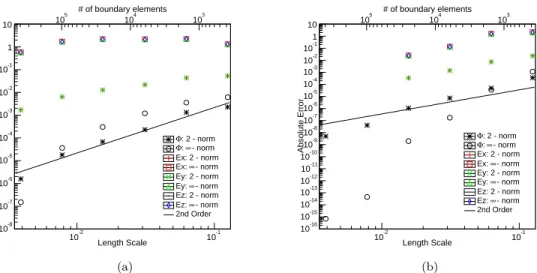
4.3 Diagram ofKSurfaceshape policies. . . 43 4.4 Diagram ofKSurface. . . 43 4.5 Computed error of the capacitance of the unit cube relative to Hwang et al. with discretized
boundary elements that are (a) equal in measure, and (b) scaled according to a power of two near the edges of the cube. Error estimates on the electric field in (b) are omitted for length scales <0.01 due to memory overflow problems related to convergence with the adaptive integrator, but trends in the global and local error of the electric field are still identifiable. . . 49 4.6 Absolute Error of the electrostatic potential and electric field for the unit cube with discretized
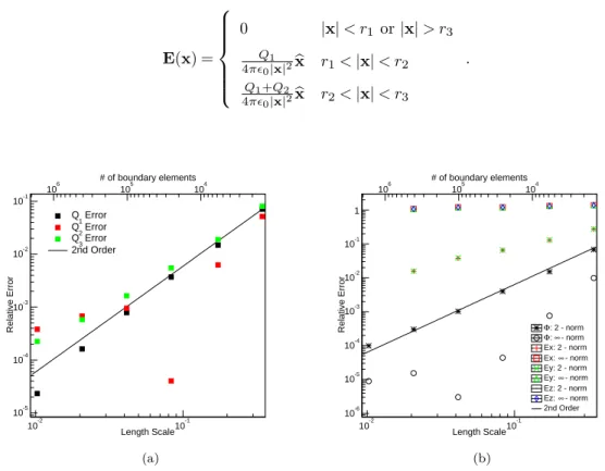
boundary elements that are (a) equal in measure, and (b) scaled according to a power of two near the edges of the cube. . . 49 4.7 Error analysis of (a) the computed charge and (b) electrostatic potential and electric field for
the spherical capacitor. Error estimates on the electric field in (b) are omitted for length scales
<0.02 due to memory overflow problems related to convergence with the adaptive integrator, but trends in the global and local error of the electric field are still identifiable. . . 51
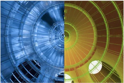
5.1 A side-by-side comparison of a photograph looking downstream inside KATRIN’s main spec-trometer (left) and its representation inKGeoBag(right). . . . 54
5.2 A CAD representation of the KATRIN FPD system, with the flux tube in green (4). In this orientation, the direction of the beam line is up and to the right. For a length scale, the pinch magnet (upstream) casing is 711 mm, and the detector magnet (downstream) casing is 910 mm. 55 5.3 (a) AKGeoBag representation of the KATRIN FPD system, and (b) an area measure of its
discretization, colored by area. The model consists of 444,821 elements. . . 57 5.4 (a)The computed charge density (scaled to accentuate small deviations from zero) and (b)
electrostatic potential (color scale) and magnetic field lines (white) in the KATRIN FPD system. . . 58 5.5 Diagrammatic representation of a Penning trap search simulation. . . 60 5.6 (a) Sampling points for a full (green) and focused (blue) Penning trap searches in the KATRIN
FPD system, and (b) the field lines corresponding to these sampling points. . . 61 5.7 Result of a Penning trap search in the KATRIN FPD system. In this image, sampling points
are assigned values according to the depth of the Penning trap at the sampling point (labeled
Gin Table 5.5 (i)). . . 62 5.8 A diagram of KATRIN’s main spectrometer, with superconducting magnets (green) at its
entrance and exit. . . 63 5.9 (a) A schematic of the use of wire arrays to improve background rejection in the main
spec-trometer (in the cylinder section of the main specspec-trometer: d1= 0.3 mm, d2= 0.2 mm, l1= 150mm,l2= 220mm,s= 25mm, δU1= 100V, δU2= 200V). Image from (5). (b) A
photograph of one of the 248 wire modules that tile the inside of KATRIN’s main spectrometer. 63 5.10 A cross-section of a wire module ring in the cylindrical section of the main spectrometer. The
5.11 A diagram of the wire module placements (rings 2−16) in KATRIN’s main spectrometer. . . 64 5.12 A diagram of KATRIN’s main spectrometer with the air coil system. The green air coils
represent the low field correction system (LFCS), and the blue, red and orange air coils denote the elements that comprise the Earth magnetic field compensation system (EMCS). Image from (6). . . 65 5.13 KATRIN’s main spectrometer, generated using KGeoBag. To reproduce the effects of the
electrodes immediately upstream and downstream from the spectrometer, additional cylinders held at ground have been added to the entrance and exit of the spectrometer. Surface elements are colored bylog10(area). . . 66
5.14 (a) A potential configuration and (b) the corresponding charge density profile for KATRIN’s main spectrometer (scaled to accentuate small deviations from zero). . . 68 5.15 Diagram of the short circuits that resulted from bake-out. Image from (7). . . 69 5.16 KGeoBag representations of the (a) full metal, (b) steep cone, (c) small flat cone, (d) middle
flat cone, (e) large flat cone and (f) cylinder wire modules. . . 70 5.17 Potential profile of the main spectrometer for (a) the nominal condition, and (b) with short
circuits. Figure (a) shows a ∆U between the inner and outer wire electrodes of 100V, while in Figure (b) ∆U= 0V. . . 72 5.18 (a) Pictorial representation of the electrostatic potential at the analyzing plane near the wire
modules for the nominal condition. For scale, the distance between the teeth of the wire module combs is 25mm. (b) Azimuthal dependence of the electrostatic potential at the analyzing plane of the main spectrometer at different fixed radii for the nominal condition. The plotted values are the differences between the potential at a field point and the potential of the inner wire electrode system. Image from (8). . . 73 5.19 (a) Pictorial representation of the electrostatic potential at the analyzing plane near the wire
modules for the shorted condition. For scale, the distance between the teeth of the wire module combs is 25mm. (b) Azimuthal dependence of the electrostatic potential at the analyzing plane of the main spectrometer at different fixed radii for the shorted condition. The plotted values are the differences between the potential at a field point and the potential of the inner wire electrode system. Image from (8). . . 74 5.20 Electrostatic potential along magnetic field lines for a magnet configuration optimized for the
nominal condition (a) in the intended nominal case, and (b) with short circuits. Magnetic field lines are colored from blue to red by increasing radius within the flux tube region. In (a), the more positive wire combs result in an increase in the electrostatic potential atz≈ ±0.9, even when partially offset by the wire comb caps. In (b), the wire combs and caps produce the opposite effect, creating two separate minima for larger radii that are no longer aligned with the minimum of the magnetic field. Images from (8). . . 74 5.21 Measured values for the center of the spectrometer vessel prior to wire installation. For
reference, the design value for the radius of the middle of the spectrometer is 4.9m. Images from (9). . . 75 5.22 Two-dimensional interpolated vessel deformation profile. Measured values are represented by
5.23 (a) East and (b) West sides of the main spectrometer model, with vessel deformation effects included (coloring only applies to the spectrometer vessel, not the ports). . . 77 5.24 Simulated potential values for the main spectrometer atz= 0,r= 3,4 mwith the deformed
vessel held at ground, and the wire system held at 1 kV. For this plot, θ= 0 corresponds to the West direction,θ=π2 corresponds to the positive vertical direction,θ=πcorresponds to the East direction, andθ=32π corresponds to the negative vertical direction. Atr= 4m
(blue), both the effects from vessel deformation and the C-profiles of the wire modules can be observed. Forr= 3m (green), the effects from individual C-profiles has diminished, and the effects from vessel deformation become the dominant perturbative effect. . . 78
6.1 (a) CAD representation of the electron gun (with the beam axis from right to left). The cylinder on the right (grey) houses the gun’s cathode and anode, and the curved section (pink) depicts the angular selection mechanism. The gun is mounted to the main spectrometer entrance magnet (aqua). Image from (10). (b) Description of electron gun parameters (αv, αh)
and the parameters used in analysis (ρgun, θgun), with origin atxm. . . 81
6.2 Simulation comparing the electron gun’s user-selected angle to the resultant pitch angle of ejected particles at the spectrometer’s entrance, for Φanode−Φcathode= 50V. Calculated for
electron starting energies which are Gaussian distributed around 0.2 eV with a sigma of 0.2 eV. Image courtesy of M. Zacher (personal communication, June 26, 2014). . . 82 6.3 Electrostatic configurations for shifted analyzing plane measurements. Configurations I through
V have a single downstream wire module ring (rings 12 through 16, respectively) held at−1kV, with the remaining rings held at−900V. For all measurements, the spectrometer vessel was held at ground. . . 83 6.4 Measured (black) and simulated (red) transmission function profiles for Run 6176. Prior to
simulation, the electron gun’s position was fit to minimize the difference in the measured and simulated energy edge for measurements corresponding to Configurations I and II (see Sec. 6.2.3). . . 93 6.5 A comparison of the measured and simulated edge fit values with respect toθgun, the angle
between the electron gun’s manipulator arm and the beam axis. Simulations were performed with the electron gun parameters described in Table 6.1. . . 94 6.6 Simulated transmission surfaces from left to right: Configuration V (blue), I (green), II
(ma-genta), III (cyan), IV (red). . . 95 6.7 Starting positions for fixed threshold andθgun for each run. The average position of
Config-urations I and II is represented by a black star. . . 96 6.8 A comparison of the measured and simulated edge fit values with respect toθgun, the angle
between the electron gun’s manipulator arm and the beam axis. Simulations were performed with the electron gun parameters described in Table 6.3. . . 97
A.1 A right triangular sub-element defined by the position of the corner opposite the hypotenuse p0, the lengths of the sides aand b, and the unit vectors in the directions of sides a andb,
labeledn1andn2. The field point is defined asp, with local coordinates (0,0, z). The corners
A.2 A non-right triangular sub-element defined by a corner p0, the length of the longest side a
and corresponding heightb, and the unit vectors in the directions of the sides connected to p0, labeled n1 andn2 (n1 always points in the direction ofa). The field point is defined as p, with local coordinates (0,0, z). The corners of the triangle are recast into local coordinates to facilitate integration. . . 110
B.1 A rectangular sub-element defined by the position of the corner opposite the hypotenusep0,
the lengths of the sidesaandb, and the unit vectors in the directions of sidesaandb, labeled n1 andn2. The field point is defined asp, with local coordinates (0,0, z). The corners of the
LIST OF ABBREVIATIONS AND SYMBOLS
AMD Advanced Micro Devices
BEM Boundary Element Method
BiCGStab method stabilized biconjugate gradient method
CAD Computer-Aided Design
CGAL Computational Geometry Algorithms Library
C.L. Confidence Level
CPU Central Processing Unit
DXF Drawing Exchange Format
EMCS Earth magnetic field compensation system
FPD Focal Plane Detector
GPU Graphical Processing Unit
KATRIN experiment Karlsruhe Tritium Neutrino experiment
LED Light Emitting Diode
LFCS low field correction system
MAC-E-Filter Magnetostatic Adiabatic Collimation followed by a Electrostatic Filter
MNS matrix Maki-Nakagawa-Sakata matrix
MPI Message Passing Interface
NERSC National Energy Research Scientific Computing Center
PDE Partial Differential Equation
PETSc Portable, Extensible Toolkit for Scientific Computation
SSC method Successive Subspace Correction method
STL Standard Template Library
UNC University of North Carolina
UV Ultraviolet
VTK Visualization Toolkit
CHAPTER 1: Introduction Section 1.1: Motivation for measurement of the neutrino mass
1.1.1: Evidence for neutrino mass from flavor oscillation
The canonical Standard Model of particle physics, a theory that has successfully predicted the experimen-tal results of almost all particle physics experiments in the past forty years, presupposes the neutrino to be massless. In the past 20 years, several experiments measuring neutrinos from the sun and from interactions in our atmosphere have uncovered compelling evidence to the contrary, linking the mass of the neutrino to an observable phenomenon known asflavor oscillation (11). In the commonly accepted 3-neutrino model of flavor oscillations, a neutrino interacts according to its flavor eigenstates (|ναi, α=e, µ, τ) and propagates
through space according to its mass eigenstates (|νii, i= 1,2,3). The mass and flavor eigenstates of a
neutrino are related by the unitary Maki-Nakagawa-Sakata (MNS) matrixUαi (12):
|νii= X
α
Uαi|ναi. (1.1)
When a neutrino is created, it is in a flavor eigenstate (|ναi). As it propagates through space, it becomes
a time-varying superposition of the three flavor eigenstates (|ν(t)i=X
α
Cα(t)|ναi) whose amplitudes
Cα(t) are determined by components of the MNS matrix, the time of propagation, the momentum of the
neutrino and the mass squared differences between neutrino mass eigenstates. Uponcharged-current weak interaction∗, the neutrino wave function interacts as one of the three flavor eigenstates with the probability
P(να)(t) =|Cα(t)|2.
In the case of two-flavor†oscillations,Uαican be represented as a simple rotation matrix dependent upon
a single mixing angleθ, and the probability of neutrino oscillation is expressed as
P(να→νβ) = sin2(2θ)×sin2
1.27∆m2
12L
E
, (1.2)
∗an interaction mediated by aW±boson
†Though there are three neutrino flavors, the two-flavor model of neutrino oscillation is useful since neutrino oscillation
where ∆m212=m21−m22is the mass squared difference of the mass eigenstates in eV2,L=c·tis the distance from the neutrino’s creation to detection in kilometers, and E is the neutrino energy in GeV (13). For three-flavor oscillations for Dirac neutrinos, there are six parameters intrinsic to the neutrino that determine is oscillatory properties: two mass squared differences (∆m2
21≃∆m2⊙, ∆m232≃∆m2atm), three mixing angles
(θ12,θ23, andθ13), and a CP violating phase (δ). The current best fit values and 3σranges for the neutrino
oscillation parameters are provided in (1), and are reproduced in Table 1.1.‘ Parameter Best fit 3σrange
δm2/10−5 eV2 7.54 6.99 - 8.18 sin2θ
12/10−1 3.08 2.59 - 3.59
∆m2/10−3 eV2 2.38 2.19 - 2.56 sin2θ13/10−2 2.40 1.78 - 2.98 sin2θ23/10−1 4.55 3.80 - 6.41 δ/π 1.31 0.98 - 1.60 (1σrange)
Table 1.1: Current best fit values and 3σranges for neutrino oscillation parameters from global 3νoscillation analysis, taken from (1). In this table, ∆m2is defined asm2
3−(m21+m22)/2,δm2is defined asm22−m21, and
an inverted neutrino mass hierarchy is assumed.
1.1.2: Significance of neutrino mass
By measuring nonzero splittings between the mass eigenstates, neutrino oscillation implies that at least two of the three neutrinos are not massless. The evidence of massive neutrinos has given rise to several interesting questions in neutrino physics theory. The three most prominent questions related to neutrino mass are:
• are neutrinosDirac (ν and ¯ν are distinct) orMajorana (ν= ¯ν) particles, • what is the ordering of the mass eigenstates, and
• what is the overall scale of the neutrino masses?
While there are several different experiments currently underway whose primary focus is to answer one of these three questions, it should be noted that the physics motivating these questions is largely interrelated, and that information about any one of these three questions will invariably shed light on the other two. As such, the Karlsruhe Tritium Neutrino (KATRIN) experiment is specifically designed to measure the overall scale of the neutrino masses, and its result will also complement the results of other neutrino experiments.
1.1.3: Current limits on the neutrino mass scale
parameters, set the sum of the three neutrino masses to be Pmν <0.23 eV (14). This constraint is
de-pendent upon the assumptions made in the cosmological model to which these parameters are fit, however. Experiments designed to measure a process known as neutrinoless double-beta decay, a process whose half-life is associated with aMajorana mass term(mββ, an incoherent sum of the electron neutrino mass states),
have set a limit onmββ to be less than 140−380 meV (15). This constraint is also model-dependent, and
would necessarily equal zero if neutrinos are Dirac particles. Finally, the current best limit on the mass of the neutrino via tritium beta decay (mβ, discussed further in Sec. 1.2.1) has been set in 2005 by the Mainz
experiment to bemβ<2.3 eV (95% C.L.) (16) and more recently by the Troitsk experiment in 2012 to be
mβ<2.05 eV (95% C.L.) (17). Measurements of this type are referred to asdirect searches, since the value
to be measured is independent of any physics model.
Section 1.2: The KATRIN experiment
The Karlsruhe Tritium Neutrino (KATRIN) experiment is a tritium beta decay experiment designed to make a direct, model independent measurement of neutrino mass with a sensitivity of mβ = 0.2 eV (90%
C.L.), an order of magnitude lower than the current limit, with a 5 sigma discovery level of 0.35 eV. To extract a neutrino mass from KATRIN one needs to understand the generation of an electron energy spectrum via tritiumβ decay, and the subsequent transport and measurement of this energy spectrum.
1.2.1: Kinematics of tritium β decay
Tritiumβ decay is described by the following reaction:
3H
→3He +e−+ ¯νe. (1.3)
Noting that ¯νeis a superposition of the three mass eigenstates, the energy spectrum of the outgoing electron
in this process is
dN
dE =C×F(Z, E)p(E+mec
2)(E
0−E)
X
i
|Uei|2[(E0−E)2−m2i] 1
2Θ(E0−E−mi), (1.4)
where E is the electron energy,me is the mass of the electron,pis the electron momentum,E0 represents
the maximum electron energy (settingmν = 0),F(Z, E) is the Fermi function (accounting for the Coulomb
function (to ensure energy conservation), and
C=G
2
F
2π3cos
2θ
C|M|2, (1.5)
whereGF is the Fermi constant,θC is the Cabibbo angle andM is the nuclear matrix element (18). Three
properties of Equation 1.4 are particularly worthy of note: first, the measurement of theβenergy spectrum is independent of whether the neutrino is Majorana or Dirac. Second, if the energy resolution of the experiment is less than the splittings between the mass eigenstates of the neutrino (as is the case for KATRIN), the massmν can be treated as a weighted average of the neutrino mass eigenstates that comprise ¯νe (19). In
other words, we can rewrite Equation 1.4 with
m2β=X
i
|Uei|2m2i (1.6)
as
dN
dE =C×F(Z, E)p(E+mec
2)(E
0−E)[(E0−E)2−m2β]
1
2Θ(E0−E−mβ), (1.7)
producing a single observable in experiment that is dependent upon all three neutrino mass eigenstates. Finally, the count rate of electrons near the end-point energy can be determined by Equation 1.4 to be proportional to (E0−E)3, which quickly approaches zero at the endpoint.
mν sensitivity = 200 meV/c2
Figure 1.1: The (A) total and (B) endpoint of the electron energy spectrum of tritiumβ decay formν= 0
eV andmν= 1 eV. The shaded region denotes the measurable difference between the massive and massless
neutrino spectra (representing only 2×10⁻¹³of the total β spectrum). Images taken from (2).
Figure 1.1, the fraction of events in the region of sensitivity to a massive ¯νe is very small: for example, only
2×10⁻¹³of the emittedβdecays account for the last 1 eV of the spectrum. The ability to accurately obtain a signal for a significantly small neutrino mass is therefore strongly dependent upon the luminosity of the tritium source, as well as the ability to precisely filter the emitted electrons below a given energy threshold‡. (3).
1.2.2: Overview of the apparatus
The KATRIN apparatus is depicted in Figure 1.2. In the Windowless Gaseous Tritium Source (WGTS), Tritium moleculesβdecay with an endpoint energy of 18.6 keV within a solenoidal magnetic field, producing an electron beam with a luminosity of 4.25×10¹⁰βs. This electron beam is transported along magnetic field lines through the differential and cryogenic pumping sections (DPS and CPS, respectively), where the residual gas molecules from the WGTS are removed, resulting in a tritium reduction factor of 1011. The beam then passes through a rough (∼100 eV resolution) and fine (∼1 eV resolution) integrating energy filter, respectively named the pre-spectrometer and main spectrometer (see Sec. 1.2.3 for a description of this filter type). Finally, the beam is deposited on a silicon pin diode detector in the detector section, designed to obtain a count rate of the β beam with a background rate≤1mHz(2)(3).
1.2.3: Measurement of the electron energy spectrum
In order to resolve the shape near the endpoint energy of the resultant electron spectrum with sufficient resolution to extract the neutrino mass, KATRIN employs an integral spectrometer known as a Magnetic Adiabatic Collimation followed by an Electrostatic Filter (MAC-E-Filter, see Fig. 1.3) (20)(21)(22). The filter is designed to adiabatically transfer a charged particle’s transverse momentum into longitudinal mo-mentum using magnetostatic fields of different strengths, and then to perform an energy rejection using electrostatic fields. For a magnetic field that varies from Bmax to Bmin and an electric potential at the
analyzing plane of U0, the transmission function of a MAC-E-Filter rises from 0 to 1 for an electron with
kinetic energyT0 as
qU0≤T0≤qU0
1 +Bmin
Bmax
, (1.8)
corresponding to a resolving power of
T0
∆T = U0
∆U =
Bmax
Bmin. (1.9)
‡Additional corrections to the spectrum shape due to the nuclear recoil and final state distributions of molecular tritium
detector region
Figure 1.2: A pictorial representation of the Karlsruhe Tritium Neutrino (KATRIN) experiment (2). The KATRIN beam line is ∼70 m long.
The relationship betweenBmax and Bmin determines the volume of the MAC-E-Filter (or, in the case of
KATRIN, the volume is also constrained by the size of the streets from the river Rhine to the experimental hall!). For the purposes of simulation, this fact is critical because it determines the large macroscopic scale intrinsic to electrostatic modeling for the KATRIN experiment. Once the filtered particles exit the spectrometer, they are collected using a silicon semiconductor detector.
1.2.4: KATRIN signal and background rates
As mentioned in 1.2.1, the integrated region of the tritiumβ spectrum that is used to fit for the neutrino mass represents a very small fraction of the entire spectrum. As a result, KATRIN requires a very intense source in order to achieve a mν sensitivity of 0.2 eV. To this end, KATRIN’s gaseous tritium source is
designed to transport 4.25×10¹⁰β per second to the entrance of the spectrometers. This rate corresponds
to a rate of∼10−2 β per second within the last eV of the energy spectrum (the shaded region in Fig. 1.1).
Another requirement for attaining KATRIN’s desired sensitivity is a relatively small background. The primary source of background in KATRIN is expected to come from particles generated within the main spectrometer, and is mitigated by a complex electrode system (see Chapter 5) and ultra-high vacuum within the vessel. With these preventative measures in place, the main spectrometer is designed to contribute backgrounds at or below 10 mHz at the tritium endpoint energy. Finally, to achieve a sufficient reduction of statistical error, the experiment is expected to take data by scanning over the endpoint of the energy spectrum, with interlaced calibration runs to monitor the stability of the apparatus, for∼3 years (23).
1.2.5: Impact on neutrino physics theory
Given the expected range of sensitivities attainable by KATRIN, either an upper limit or a definitive measurement of the neutrino mass will yield important results to determining the nature of neutrino mass. If a value for the mass mν can be determined, we will be able to fix the absolute mass spectrum of the
mass eigenstates. Because the splittings of the mass eigenstates are an order of magnitude smaller than the expected sensitivity of KATRIN, the reconstructed neutrino mass will be a weighted average of the three mass eigenstates according to Equation 1.6 and, while not sensitive to mass ordering, would determine that the neutrino masses are nearly degenerate. Such a measurement could also be used in tandem with 0νββ
Section 1.3: Electromagnetic simulations in the KATRIN experiment
1.3.1: Boundary Element Method
To characterize the properties of its particle transport and filtering apparatus, an accurate simulation of KATRIN’s electromagnetic fields is required. To achieve this goal, we have developed a Boundary Ele-ment Method (BEM) for converting three-dimensional boundary value problems in potential theory into a numerically soluble linear algebraic form. A description of this technique is given in Chapter 2.
1.3.2: Robin Hood linear algebraic solver
As a result of the large range of length scales inherent in KATRIN’s transport and spectrometer system, the linear algebraic equations generated by our BEM can quickly become very large (resulting in dense square matrices with rank∼106). To solve these systems of equations, we have employed a novel quasi-stationary Robin Hood linear algebraic solver, and adapted it to perform in high-performance computing environments. The Robin Hood linear algebraic solver is described in greater detail in Chapter 3.
1.3.3: Electromagnetic simulation software
Following the theoretical description of the BEM and Robin Hood solver, Chapter 4 provides a descrip-tion of their implementadescrip-tion in theKEMFieldsoftware. We also briefly presentKGeoBag, software designed to describe the complex geometries inherent in the KATRIN experiment. In some respects, KGeoBag has been designed to operate as a front-end toKEMField: KGeoBagaccepts user-defined descriptions of macro-scopic geometry elements and provides navigation, discretization and visualization routines for them. These elements are then passed into KEMField, whose primary focus is the high-performance computation of the BEM and subsequent field queries.
1.3.4: Application to the KATRIN experiment
With the aforementioned software tools in place, Chapter 5 exhibits the application of KGeoBag and
1.3.5: Shifted analyzing surfaces
Finally, to validate our model of KATRIN’s main spectrometer, in Chapter 6 we present an analysis of measurements taken during KATRIN’s spectrometer commissioning, where the electrostatic configuration of the main spectrometer was adjusted to shift its analyzing surface away from the center of the vessel. To do this, we first present a technique for simulating the transmission function from a point-like electron gun source. We then compare the results of simulation to their empirical counterparts.
Section 1.4: Summary
CHAPTER 2: Boundary Element Method Section 2.1: Introduction
The Boundary Element Method (BEM) is a technique for numerically solving linear partial differential equations (PDEs) that can be represented as an integral over the domain boundary. Compared to other popular methods like the Finite Element and Finite Difference Methods, the BEM requires that all source terms reside on the system’s boundaries, rather than its interior (25). This restricts the applicability of the technique to a subset of PDEs, but also reduces the dimensionality of the problem and facilitates the calculation of fields for regions that extend out to infinity (rather than restricting computation to a finite region) (26). These two features make the BEM more favorable than competing methods when it is applicable.
The method involves taking an integral equation that describes a field as a function of its boundaries, and feeding the boundary conditions into the equation in order to construct a profile for the unknown function in the integrand. Typically, the integral equation is a Fredholm integral equation of the first or second type, defined respectively as
f(x) =
Z
Γ
K(x, x′)ϕ(x′)dx′ (2.1)
and
ϕ(x) =f(x) +λ
Z
Γ
K(x, x′)ϕ(x′)dx′, (2.2)
where K(x, x′) (known as the Fredholm kernel) and f(x) are known, square-integrable functions, λ is a constant, Γ is the system’s boundary andϕ(x) is the function for which we are trying to solve (27).
Many variants of the BEM exist. The version described here is known as an indirect Boundary Element
Method, as the technique emphasizes matching the solution function’s values or derivatives across domains
that share a common boundary. This is in contrast to direct Boundary Element Methods, which use the complete specification of the boundary of a single region to obtain a description of the function in that region∗.
∗The termdirectrefers to the act of directly solving for a function’s boundary derivative values from the function’s boundary
Section 2.2: Conversion of the Laplace Equation to a Fredholm integral equation
2.2.1: Description of the Laplace Equation
The governing partial differential equation for electrostatic systems is the Laplace equation:
∇2φ= 0. (2.3)
The Laplace equation admits a unique solution whenφis defined on all boundary surfaces (Dirichlet bound-ary conditions), ∂φ∂n is defined on all boundary surfaces (Neumann boundary conditions)†, or an admixture ofφand ∂φ∂n are defined along the entire boundary (mixedboundary conditions).
To apply the BEM to electrostatics we will convert Equation 2.3 into a Fredholm integral equation of the first type (see Eq. 2.1). We must also ensure that the resulting Fredholm kernel is square-integrable. The following technique is derived from the methods described in (28)(29)(30)(31)(32)(33), and is described in 3 dimensions (with 2-dimensional accompanying images).
2.2.2: Integral Statement for the Interior Equation
Σ
x
Figure 2.1: A graphical depiction of the region Σ and observation pointxwith dimensionalityd= 2.
We begin by defining a volume Σ, bounded by a piecewise smooth closed and positively oriented contour (see Fig. 2.1). We apply Green’s second identity to Σ:
Z
Σ
u∇2w+w∇2udV =
Z
∂Σ
u∂w
∂n−w
∂u ∂n
dS, (2.4)
where u, w:R3→R are C2 continuous in Σ and on its boundaries ∂Σ, and ∂w
∂n is the magnitude of the
gradient ofwin the direction of the outward pointing normalnto the surface elementdS‡. We letube the
†Neumann boundary conditions uniquely specify a solution up to an additive constant.
‡We define C2 continuity for a function f(
x) on V ∪∂V in the limiting sense: ∀x∈V ∪∂V,y∈V, limy→xf(x) and limy→x
∂f(x)
solution to Equation 2.3, eliminating one of the terms on the left-hand side of Equation 2.4 and leaving us with
Z
Σ
φ∇2wdV =
Z
∂Σ
φ∂w
∂n−w
∂φ ∂n
dS. (2.5)
Next, we choose a suitablewto eliminate the remaining domain integral on the left-hand side of Equation 2.5, so that only calculations around the boundaries of Σ remain. This is done by casting the left-hand side as a singular integral whose kernel is the fundamental solution of the Laplace equation, G:R3×R3→R,
defined by the property
∇′2G(x,x′) =δ(x−x′), (2.6)
and one of whose arguments is an (often implied)observation pointx∈R3. In 3 dimensions, the fundamental
solution to the Laplace equation is
G(x,x′) = 1
4π|x−x′|. (2.7)
Immediately, it can be seen that our choice ofwhas introduced singularities that could potentially prevent our final Fredholm kernel from being square integrable. It is therefore necessary to address the singularities in Equation 2.5 whenx=x′, both in Σ and on its boundaries.
2.2.3: Resolving Singularities with Limiting Behaviors
Our approach to dealing with singularities in Equation 2.5 is to excise a parametrized volume containing our observation point (hereafter referred to as Ex(ǫ)) from our domain, Σ, so our equations become
inte-grable. We then observe the behavior of our equations in the limit that the parametrized volume vanishes. We begin by dealing with the singularity that occurs whenx=x′, andx∈Σ. For this condition, we excise
Σ
Ε
x(
ε
)
Figure 2.2: By excluding a small Ex(ǫ), we are able to avoid the divergence in Eq. 2.5 whenx=x′, and
x∈Σ. Taking the limit asǫ→0, we recover our original domain.
ǫ >0 (see Fig. 2.2). This results in a modification of Equation 2.5 to
Z
Σ\Ex(ǫ)
φ∇2GdV =
Z
∂Σ
φ∂G
∂n−G
∂φ ∂n
dS−
Z
∂Ex(ǫ)
φ∂G
∂n−G
∂φ ∂n
dS. (2.8)
The left-hand side of this equation is then trivially zero (since ∀x′∈Σ\Ex(ǫ)⇒ ∇′2G(x,x′) = 0), and
Equation 2.8 reduces to
Z
∂Σ
φ∂G
∂n−G
∂φ ∂n
dS=
Z
∂Ex(ǫ)
φ∂G
∂n−G
∂φ ∂n
dS. (2.9)
To evaluate the right-hand side of Equation 2.9, we convert into a local spherical coordinate system centered on our observation point:
x′−x ≡ ρ(ρ, θ, ϕ),
n = ρ
|ρ|,
dS = ǫ2dΩ. (2.10)
We evaluate the first term on the right-hand side to be
Z
∂Ex(ǫ)
φ(x′) ∂
∂nG(x,x
′)
·dS =
Z
∂Ex(ǫ)
φ(x+ρ)· ∂ ∂ρ
1 4πρ
·dS=
=
Z
Ω
dΩ·ǫ2·φ(x+ρ)·
−4πǫ12
= = − 1
4π
Z
Ω
dΩ·φ(x+ρ), (2.11)
which, asǫ→0, approaches−φ(x). The second term on the right-hand side of Equation 2.9 becomes
Z
∂Ex(ǫ)
G(x,x′) ∂
∂nφ(x
′)
·dS =
Z
∂Ex(ǫ)
1 4πρ
·∂ρ∂ φ(x+ρ)·dS
= ǫ
4π
Z
Ω
dΩ· ∂
∂ρ(φ(x+ρ)|ρ=ǫ, (2.12)
which approaches 0 asǫ→0, since we are guaranteed that ∂ρ∂ φ(x+ρ) is well-behaved by the earlier
require-ment that∀x′∈Σ :φ(x′) be twice continuously differentiable. We therefore determine that the right-hand side of Equation 2.5 converges toφ(x) whenx=x′,x∈Σ.
Σ
Ε
x(
ε
)
x
Ωx
Figure 2.3: Whenx=x′,x∈∂Σ, we exclude a partial sphereEx(ǫ) with interior solid angle Ωxto eliminate
the divergence in Eq. 2.5. Taking the limit asǫ→0, we recover our original domain.
spherical portion of∂Ex(ǫ), andSxΣ(ǫ) to be the portion of∂Ex(ǫ) along∂Σ (see Fig. 2.3)§. This excision
changes Equation 2.5 to be
Z
Σ\Ex(ǫ)
φ∇2GdV =
Z
∂Σ\SΣ
x(ǫ)
φ∂G
∂n−G
∂φ ∂n
dS−
Z
SΩ
x(ǫ)
φ∂G
∂n−G
∂φ ∂n
dS. (2.13)
Once again, the left-hand side of Equation 2.13 evaluates to 0, leaving us with
Z
∂Σ\SΣ
x(ǫ)
φ∂G
∂n−G
∂φ ∂n
dS=
Z
SΩ
x(ǫ)
φ∂G
∂n−G
∂φ ∂n
dS. (2.14)
We convert to a local spherical coordinate system as prescribed in Equation 2.10 and evaluate the first term on the right-hand side of Equation 2.15 to be
Z
SΩ
x(ǫ)
φ(x′) ∂
∂nG(x,x
′)
·dS =
Z
SΩ
x(ǫ)
φ(x+ρ)· ∂ ∂ρ
1 4πρ
·dS=
= ǫ2
Z
Ωx
dΩ·φ(x+ρ)·
−4πǫ12
= = − 1
4π
Z
Ωx
dΩ·φ(x+ρ), (2.15)
which, asǫ→0, approaches−Ωx
4π ·φ(x). The second term on the right-hand side of Equation 2.13 becomes Z
SΩ
x(ǫ)
G(x,x′) ∂
∂nφ(x
′)
·dS =
Z
SΩ
x(ǫ)
1 4πρ
·∂ρ∂ φ(x+ρ)·dS
= ǫ
4π
Z
Ωx
dΩ· ∂
∂ρ(φ(x+ρ)|ρ=ǫ, (2.16)
which tends to 0 as ǫ→0, since since we are once again guaranteed that ∂ρ∂φ(x+ρ) is well-behaved by
§Ifxis on a smooth contour, Ωx= 2π. Otherwise, Ωxis dependent upon theC1 discontinuity of the piecewise-continuous
the earlier requirement thatφ(x) be twice continuously differentiable. We have therefore shown that, when x=x′,x∈∂Σ, the right-hand side of Equation 2.5 converges to Ωx
4π·φ(x).
2.2.4: Final form of the Interior Equation
Having demonstrated thatG(x,x′) is square-integrable∀x∈R3, we now formulate an expression for the
solution to the Laplace equation in Σ as an integral equation:
c(x)·φ(x) =
Z
∂Σ
φ(x′)∂G(x,x ′)
∂n −G(x,x
′)∂φ(x′)
∂n
·dS, (2.17)
c(x) =
1 x∈Σ
Ωx
4π x∈∂Σ
0 x∈/Σ
. (2.18)
Up to this point, our derivation has held valid for the treatment for both the direct and indirect Boundary Element Methods. To proceed with a direct formalism, Equation 2.17 would be used to compute source terms given appropriate boundary conditions, and an equation would be obtained that is valid∀x∈Σ. With a little more manipulation, however, the indirect approach yields a much more general solution that is valid ∀x∈R3.
2.2.5: Extension to the Exterior Equation
Σ
x R
S (R)1
~
Σ
Figure 2.4: A graphical depiction ofΣ in 2 dimensions.e
Equation 2.5 forΣ:e
Z
e
Σ
e
φ∇2GdV =
Z
∂eΣ
e
φ∂G
∂n−G
∂φe ∂n
!
dS. (2.19)
It is important to note that, as a consequence of the choice of boundary orientation, we have defined
∂Σ =e S2(R)∪(−∂Σ). By requiring that
lim |x|→∞
e
φ(x) = lim |x|→∞
∂φe ∂n x
= 0, (2.20)
we can impose the condition that S2(R) have no contribution to the right-hand side of Equation 2.19 by
extending R→ ∞. Subsequent application of the procedure described in Section 2.2.3 yields the following integral equation:
e
c(x)·φe(x) =
Z
∂eΣ
e
φ(x′)∂G(x,x ′)
∂n −G(x,x
′)∂φe(x′)
∂n
!
·dS, (2.21)
e
c(x) =
1 x∈Σe
1−Ωx
4π x∈∂Σe\S2(R)
0 x∈/Σe
, (2.22)
and the subtended solid angle Ωxhas been defined earlier (see Fig. 2.3). With care to preserve the correct
boundary orientations, we can rewrite Equation 2.21 in terms of our original region Σ and its boundary:
e
c(x)·φe(x) =−
Z
∂Σ
e
φ(x′)∂G(x,x ′)
∂(n) +G(x,x
′)∂φe(x′)
∂(−n)
!
·dS (2.23)
ec(x) =
0 x∈Σ
1−Ωx
4π x∈∂Σ
1 x∈/Σ
. (2.24)
2.2.6: Composing a Global Solution
We now have two distinct regions (Σ,Σ) that share a common boundary, each with a solution functione (φ,φe) dependent on the properties of the boundaries of our system. With this, We can compose a global solution function Φ that spans both regions by enforcing a boundary matching condition between our solu-tions. Our two choices are to enforce a relationship betweenφand φeand solve for a source termσ defined by the discontinuities between ∂φ∂n and ∂(∂−eφn), or to enforce a requirement on the derivatives and solve for a source termµdefined by a discontinuity betweenφandφe. The two choices result in asingle-layer potential
that extends more naturally to a physical description within the field of electrostatics. By enforcing a C0 continuity condition betweenφandφealong∂Σ:
φ(x) =φe(x) ∀x∈∂Σ, (2.25)
and defining our globally defined composite function Φ as
Φ(x) =
φ(x) x∈Σ∪∂Σ
e
φ(x) x∈/Σ
, (2.26)
we can add Equations 2.17 and 2.23 to obtain a global integral equation:
Φ(x) =−
Z
∂Σ
G(x,x′) ∂φ(x
′)
∂n +
∂φe(x′)
∂(−n)
!
·dS. (2.27)
Since we are treating the discontinuity of the derivatives at the boundary as an independent function, we can defineσ(x),x∈∂Σ as
σ(x) =− ∂φ(x)
∂n +
∂φe(x)
∂(−n)
!
, (2.28)
and rewrite Equation 2.27 as
Φ(x) =
Z
∂Σ
G(x,x′)·σ(x′)·dS. (2.29)
Now that we have Equation 2.29, we need to incorporate the boundary conditions that uniquely define our solution function Φ.
2.2.7: Application of Boundary Conditions
As mentioned in Section 2.2.1, our solution function Φ is uniquely described by imposing Dirichlet, Neumann or mixed boundary conditions on the boundaries of our system. To apply a Dirichlet boundary condition, we simply restrict the domain of Equation 2.29 to our boundary:
∀x∈∂Σ : Φ(x) =
Z
∂Σ
G(x,x′)·σ(x′)·dS (2.30)
to have discontinuous derivatives at the boundary. Using our convention of defining the function as a limit to the boundary, we therefore obtain two different formulae for this derivative as we approach from within Σ or without:
∀x∈∂Σ,y+∈Σ : ∂Φ(x)
∂n
+= limy+→x
∂Φ(y+)
∂n =
Z
∂Σ\x
∂G(x,x′)
∂n ·σ(x
′)
·dS−Ωx
4π·σ(x), (2.31)
∀x∈∂Σ,y−∈/Σ : ∂Φ(x)
∂n
−= limy−→x
∂Φ(y−)
∂n =
Z
∂Σ\x
∂G(x,x′)
∂n ·σ(x
′) ·dS+
1−Ω4πx
·σ(x), (2.32)
where we have adopted the convention of±being the limit taken along or away from the boundary normal, respectively.
With Equations 2.31 and 2.32, we can enforce a relationship between the derivatives at either side of the boundary. For example, the condition
ǫ+· ∂Φ(
x) ∂n +
=ǫ−· ∂Φ( x) ∂n − (2.33)
yields the following integral equation:
σ(x) =
Z
∂Σ\x
ǫ+−ǫ−
Ωx
4πǫ++
1−Ωx
4π
ǫ−
·∂G(x,x′)
∂n ·σ(x
′)
·dS, (2.34)
which is a Fredholm equation of the second kind.
A mixed boundary condition is simply the discrete combination of Dirichlet and Neumann boundary conditions along∂Σ. As such, we can solve problems of this type by applying Equations 2.30 and 2.34 to the Dirichlet and Neumann sections of the boundary, respectively. This is explained in more detail in Section 2.4.
2.2.8: Extension to Multiple Regions and Disjoint Boundaries
Although we have derived our integral equations using a single boundary enclosing a volume, this method is immediately extensible to the partitioning of space into multiple regions that share boundaries. Doing so would simply result in an integral equation for each region of space, with the requirement that the solution function be a composite of these solutions that is C0 continuous across each boundary. The final integral
equation is given as
∀x∈[
j
∂Σj: Φ(x) = X
j Z
∂Σj
G(x,x′)·σ(x′)·dS. (2.35)
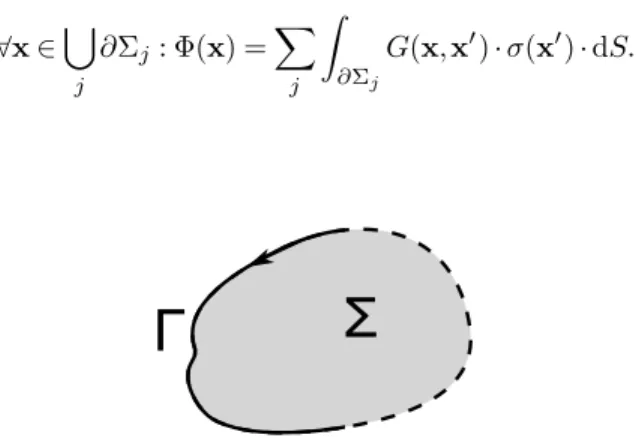
Σ
Γ
Figure 2.5: A disjoint boundary Γ (solid black line), and a constructed space Σ partially bound by Γ. The remaining boundary∂Σ\Γ (dashed black line) can be assigned thenull boundary condition defined in Eq. 2.36, allowing us to apply our formalism on a closed contour.
The resulting derivation can be extended to accommodate systems with disjoint boundaries as well. To demonstrate this, we can connect disjoint boundaries with an artificial boundary that enforces a continuity of the derivatives on either side of a boundary segment:
∂Φ(x)
∂n
+
= ∂Φ(x)
∂n
−
. (2.36)
It can be seen from Equations 2.31 and 2.32 that the application of thisnullcondition to a boundary segment enforces thatσ(x) = 0 in this region. To apply our formalism to a disjoint boundary, we can construct a space that is partially bound by a disjoint boundary, and define the remainder of its boundary to have this null boundary condition (see Fig. 2.5). In practice this is obviously not necessary; we can apply our boundary integral equations to these disjoint boundaries without any extra work.
Section 2.3: Discretization of Fredholm Integrals for Numeric Computation
Now that we have constructed Fredholm integrals to represent the Laplace equation with both Dirichlet boundaries (Equation 2.30) and Neumann boundaries (Equation 2.34), we describe a technique for solving these equations.
2.3.1: Dirichlet Boundaries
Equation 2.1 so that Γ =Pj∆Γj, and then recast the equation as
f(x) =X
j Z
∆Γj
K(x,x′)·ϕ(x′)·dS. (2.37)
Applying a Collocation Scheme
We approximate a solution for ϕto second order accuracy with respect to the length scale of ∆Γj using
a zeroth-order collocation scheme, which approximates ϕ as a piecewise-constant function defined on our
boundaries. To do this, we first use the fact that the average of a smooth function f(x) over a surface Γ is approximated to the second order of the length scale of Γ by its evaluation at the geometric mean of the surface (34):
hf(x)iΓ≡ 1 |Γ|·
Z
Γ
f(x′)·dS=f(x0) +O(|Γ|), (2.38)
where|Γ|is the area measure of the surface Γ,
x0≡
R
Γx
′dS
|Γ| (2.39)
is the centroid of Γ, and the truncation errorO(|Γ|) scales with the square of the maximal distance of a pointx∈Γ fromx0:
O(|Γ|)≡ O |x−x0|2. (2.40)
We also note that the product of the average of two functions is equal to the average of the product of the functions to second order, since
hf(x)iΓ· hg(x)iΓ = (f(x0) +O(|Γ|))·(g(x0) +O(|Γ|)) =
= f(x0)·g(x0) +O(|Γ|) =
= hf(x)·g(x)iΓ+O(|Γ|). (2.41)
To affect our collocation scheme, we first convert the integral overx′ in Equation 2.37 into an average over ∆Γj:
f(x) =X
j
We then expand the averaged term in Equation 2.42 using Equation 2.41:
f(x) = X
j
|∆Γj| ·K(x,x′)
∆Γj·
ϕ(x′)∆Γ
j+O(|∆Γj|)
=
= X
j
|∆Γj| ·K(x,x′)∆Γj·ϕ(x′)∆Γj+O |∆Γj|2. (2.43)
Next, we substitute an approximation tohϕ(x′)i∆Γj as defined in Equation 2.38:
f(x) = X
j
|∆Γj| ·K(x,x′)∆Γj· ϕ(xj) +O(|∆Γj|)+O |∆Γj|2=
= X
j
|∆Γj| ·K(x,x′)∆Γj·ϕ(xj) +O |∆Γj|2, (2.44)
where xj is the centroid of ∆Γj as defined by Equation 2.39. ConvertinghK(x,x′)i∆Γj back into integral
form, we arrive at our collocated equation:
f(x) =X
j Z
∆Γj
K(x,x′)·dS
!
·ϕ(xj) +O |∆Γj|2. (2.45)
If we assume that,∀j,|∆Γj| ≈ǫ2(whereǫis the average length scale of our surfaces), the summation of the
error terms in Equation 2.45 results in an overall collocation error ofO ǫ2:
f(x) =
X
j Z
∆Γj
K(x,x′)·dS
!
·ϕ(xj)
+O ǫ2. (2.46)
Discretizing the Boundary
Equation 2.46 provides us with a means to compute field values given a piecewise-constant solution forϕ, but we still must solve forϕ. This is accomplished by converting Equation 2.46 into a discrete set of soluble equations, using known values off(x). The natural choice for these known field values are the centroids of ∆Γi:
f(xi) =X
j Z
∆Γj
K(xi,x′)·dS
!
where the error estimate has been omitted for the sake of clarity. By affecting the following change in notation:
f(xi) → fi, (2.48)
Z
∆Γj
K(xi,x′)dS → Kij, (2.49)
ϕ(xj) → ϕj, (2.50)
to Equation 2.47, we arrive at the following relation:
fi= X
Kijϕj, (2.51)
in whichϕj can be solved using one of many computational linear algebraic techniques.
2.3.2: Neumann Boundaries
The procedure for the Neumann condition is analogous to that for the Dirichlet condition, applied to the Fredholm integral equation of the second kind (Equation 2.2). We discretize our region of integration:
ϕ(x) =f(x) +λX
j Z
∆Γj
K(x,x′)ϕ(x′)dS, (2.52)
apply our collocation scheme and discretize our boundary¶:
ϕ(xi) =f(xi) +λ X
j Z
∆Γj
K(xi,x′)·dS !
·ϕ(xj), (2.53)
and recast into a linear algebraic equation:
fi= X
Kijϕj, (2.54)
where
fi = f(xi),
Kij = −λ·
Z
∆Γj
K(xi,x′)dS+δij,
ϕj = ϕ(xj). (2.55)