Sharif University of Technology
Scientia IranicaTransactions D: Computer Science & Engineering and Electrical Engineering http://scientiairanica.sharif.edu
Research Note
Lyapunov-global-Lanczos algorithm for model order
reduction and adaptive PI controller of large-scale
electrical systems
M. Kouki
, M. Abbes, and A. Mami
Universite de Tunis El Manar, Institut Superieur d'Informatique et de Gestion de Kairouan, LR-11-ES20 Laboratoire Analyse, Conception et Commande des Systemes, BP 37, LE BELVEDERE 1002, Tunis, Tunisie.
Received 15 February 2016; received in revised form 15 August 2016; accepted 22 April 2017
KEYWORDS Lanczos; Lyapunov; Model order reduction; Adaptive PI; Gl obal Lanczos; ARDUINO.
Abstract. Mathematical modeling of complex electrical systems has led us to linear mathematical models of higher order. Consequently, it is dicult to analyze and to design a control strategy for these systems. Order reduction is an important and eective tool to facilitate the handling and designing of a control strategy. In this paper, we rstly present a reduction method, which is based on the Krylov subspace and Lyapunov techniques, called Lyapunov-Global-Lanczos. This method minimizes the H1norm error and absolute error,
and preserves the stability of the reduced system. It also provides a better reduced system of order 1, with closer behavior to the original system. This rst order system is used to design PI (Proportional-Integral) controller. Secondly, we implement an adaptive digital PI controller in a microcontroller. It calculates the PI parameters in real time, referring to the error between the desired and measured outputs and the initial values of PI controller, that are determined from the rst order system. Two simulation examples and a real-time experimentation are presented to show the eectiveness of the proposed algorithms. © 2018 Sharif University of Technology. All rights reserved.
1. Introduction
Design, realization, and synthesis of a control diagram of a complex electrical system are most often the rst and most delicate tasks in industry. In the last 30 years, the emergence of modeling and digital simulation has allowed to greatly reduce the cost and time spent in design phases. In contrast, system validation phases remain critical as they arrive late in the design cycle. The exact numbers dier depending on the study, but the cost of correction of an error detected at the stage of testing is very much higher than the cost of correcting
*. Corresponding author.
E-mail address: [email protected] (M. Kouki) doi: 10.24200/sci.2017.4368
an error in the specication phase. The industries seek to involve the validation phases earlier and earlier in the design cycle. However, in the early design phases, systems are modeled on specic simulation platforms. Hardware connection with physical modeling platforms requires to perform real-time simulations. However, the real-time constraint requires simulation results to be delivered as accurate as possible within imposed deadlines. Thus, the produced model is character-ized by high complexity and this may require higher computing time than the available time. In this case, cost constraints usually lead to the interest in the use of model reduction methods. When the system is described by dierential linear equations, simplication can be carried out by reducing the order of the model. Order reduction in models reduces the complexity of the model while preserving the majority of the
input-output behavior. In addition, the use of simplied methods intervenes in the design of a suitable control strategy with complex real systems. To design an eective controller for high order electrical process, we need to reduce the mathematical model of the real process. In the past decade, the controller mostly used in processing in the industries has been the PI/PID (Proportional-Integral Derivative) (in more than 90% of the whole control loop). PI is a valuable tool that has many advantages over the other controllers, including simple design, high reliability, robustness, numerical stability, and digital implementation simplicity in prac-tice. However, when designing a PI control strategy in a high order system, it is necessary to choose the most reliable reduction method, which provides a system of order 1 having frequency and time responses that are the nearest to the original system response and having a transfer function of order 1, whose numerator value is close to 1.
In this work, we propose a reduction method ap-plied to large-scale electrical systems. Our method ben-ets from both Krylov [1] and Lyapunov techniques [2-4]. The proposed method generates models of reduced order with similar behavior to the original system, leading to minimized absolute error and H1norm error
and preserving the stability of the reduced system. We also present an adaptive control algorithm, which we call adaptive digital PI controller, implemented in a microcontroller to monitor, in real time, a large-scale real system. This algorithm determines the appropriate parameters of PI controllers in real time based on the error between the desired output and the measured one, and the initial controller parameters are determined from a reduced system (order 1).
The mathematical problem of electrical system can be stated as follows.
Consider a class of descriptor linear dynamical electrical system in state space form given by [5-8]:
=
Edx(t)dt = Ax(t) + Bu(t)
y(t) = Cx(t) + Du(t) (1) where E 2 Rnn, A 2 Rnn, B 2 Rn1, C 2 R1n,
D 2 R11, u(t) 2 R, and y(t) 2 R, such that E is not
an identity matrix.
After applying the Laplace transform to System (1), the transfer function of the original descriptor linear system is given by [9-12]:
f(s) = C(sE A) 1B + D: (2)
The problems consist of:
Constructing the parameters of the reduced descrip-tor linear dynamical system : Em 2 Rmm, Am 2
Rmm, B
m2 Rm1, Cm2 R1m, Dm2 R11, and
ym(t) 2 R, where m n is the order of reduced
system.
The state space representation of reduction descriptor linear dynamical systems is as follows [9]:
m=
Emdxmdt(t) = Amxm(t) + Bmu(t)
ym(t) = Cmxm(t) + Dmu(t) (3)
The Laplace transform is applied to System (3); hence, the transfer function of the reduced descrip-tor linear system is as follows:
fm(s) = Cm(sEm Am) 1Bm+ Dm: (4)
Determining a real-time adaptive digital PI con-troller based on the concon-troller parameters deter-mined by the reduced system in such a way that it guarantees the eectiveness by giving the best values of kp and ki gains according to the real time change
of the input. The transfer functions of the initial controller and the adaptive one are, respectively, presented as follows:
Gc(s) = kp+ksi ) ^Gc(s) = ^kp+^ksi; (5)
where, kp and ki are, respectively, the proportional
and integral gains, which were determined by the reduced system. ^kp and ^ki are, respectively, the
proportional and integral tuning gains obtained in real-time experimentation.
This paper is organized as follows. In Section 2, we present some basic mathematical tools. In Sections 3 and 4, we present our reduction approach and apply it to two theoretical systems of dierent orders. In Section 5, our adaptive control algorithm will be pre-sented and applied to a real electrical system. Section 6 concludes the work.
2. Basic tools
In this section, we will review some basic mathematical tools, standard Krylov subspace, Lyapunov technique, and H1norm error.
2.1. Standard Krylov subspace
Let a square matrix be A and a vector be b; apply the Krylov subspace technique. The standard Krylov subspace, KmfA; bg, such that m is its dimension is
obtained by [13-15]:
KmfA; bg = spanfb; Ab; :::; Am 1bg: (6)
2.2. Lyapunov equations
Let an asymptotically stable descriptor linear system be as in Eq. (1). The Lyapunov solution to this
system is obtained by solving the following system (Eq. (7)) [10,16]:
ARc+ RcAT + BBT = 0
ATRo+ RoA + CTC = 0 (7)
The solutions to this system are Rc and Ro[10]. Rc2
Rnn and R
o 2 Rnn are called the reachability and
the observability Gramian matrices, respectively. 2.3. H1 errors of dynamical descriptor linear
systems
The global error bound between the original system and the reduced one is obtained by computing H1
norm error knowing that [10,11,17]:
kf(jw) fm(jw)kH1=supw2Rkf(jw) fm(jw)k2:
(8)
3. Lyapunov-Global-Lanczos method of linear descriptor system
The Lyapunov-Global-Lanczos (Lyap-GL) method is an extension of the Global Lanczos (GL) method [18]. It is based on generation of two projection matrices, V and W 2 Rnm. The V projection matrix is
generated by the use of the Krylov subspace technique and the W projection matrix is determined by the use of the Lyapunov and Krylov subspace techniques. The Krylov technique is used for its numerical eciency and the Lyapunov one is used because of its robustness in determining the observability Gramian matrix.
Lyap-GL minimizes the H1error, absolute error,
and the error between the time responses of original and reduced systems and preserves the stability of the reduced system independently of its order. The two projection matrices satisfy a bi-orthogonality condition (Eq. (9)):
(W (((WT V ) 1)T))TV = I: (9)
The numerical eciency is caused by the use of Krylov subspace technique [18]. The use of the observability Gramian matrix in generating the second subspace W has numerous advantages that are:
Minimization of the error between the original sys-tem and the reduced one in frequency response;
Minimization of the error between the original sys-tem and the reduced one in time response;
Minimization of the H1 norm error;
Stability preservation;
Passivity preservation.
Theorems 1 and 2 summarize the principles of our approach.
Theorem 3.1. (Generation of V matrix)
Let = (s1E A) 1E be non-singular matrix
and = (s2E A) 1Ro1 be a vector (where s1
and s2 are expansion points). The Krylov subspace,
Km(; ) = f; ; :::; m 1g, is generated using the
Krylov technique. It satises the recurrent relationship (Eq. (10)):
Vm= VmTm+ m+1vm+1eTm; (10)
where, em is the mth unit vector of identity matrix
and Tm = WmVm is a tridiagonal matrix, which is
composed of the scalars i=
q
trace(abs(RT
oi)), below
the diagonal, i = trace(RToivi) on the diagonal, and
i= itrace(abs(RToi)) above the diagonal (where, i =
1 : m).
Proof 1. The proof can be found in [19,20]
Theorem 3.2. (Generation of W matrix) Let T be nonsingular matrix and r = Ro1
1 . The
Krylov subspace, Lm(T; r), is generated by applying
the Krylov technique. It is dened as in Eq. (11): Lm(T; r) = spanfr; Tr; :::; (m 1)Trg: (11)
The Krylov subspace satises the recurrent Eq. (12): TW
m= WmTmT+ m+1wm+1eTm: (12)
Proof 2. The proof can be found in [9,10]. Table 1 explains the algorithm of Lyapunov-Global-Lanczos approach. The main steps of our approach are:
Step 1: Generate the observability Gramian matrix, Ro;
Step 2: Compute the matrix and the vector ; we use the rst column of observability Gramian matrix in computing ;
Step 3: Compute the rst scalars 1, 1, and 1 by
the use of the observability Gramian matrix;
Step 4: Generate the second vector of V and of the modied observability Gramian matrix Ro (also
called W second projection matrix) based on the pre-vious vectors of two projection matrices, the scalars coecient of T matrix, and the original observability Gramian matrix;
Step 5: Compute the parameters of reduced system using the congruence transformation:
Em= (W (((WT V ) 1)T))T E V;
Am= (W (((WT V ) 1)T))T A V;
Table 1. Lyapunov-global-Lanczos algorithm. Inputs: A, B, C, D, E, s1, s2; Outputs: V, W
(1) Generate the observability Gramian matrix Ro by using of the Lyapunov technique:
ATR
o+ RoA + CTC = 0
(2) Initialization:
(a) Compute the matrix and the vector , that will be used in the generation of Krylov subspace: Set = (s1E A) 1E and = (s2E A) 1Ro1
(b) Compute the initial coecients and of T matrix: 1=ptrace(abs(RTo1))
1= 1trace(abs(RoT1)) (c) Dene:
v1 =1
w1=Ro11
(d) Compute the initial coecient of T matrix: 1= trace(RTo1v1)
(3) Generate the two projection matrices V and W : for i = 1 : m
(a) Compute the vi+1vector of V :
vi+1= vi ivi vi 1
(b) Compute the wi+1vector of W :
wi+1= T Roi iRoi Roi 1 (c) Update and
i+1=
q
trace(abs(vi+1wi+1T ))
i+1= i+1trace(abs(wTi+1vi+1))
(d) Compute the normalized vectors vi+1and wi+1:
vi+1=vi+1i+
Roi+1=wi+1i+1
(e) Compute the other coecient of T matrix: i+1= trace(RToi+1vi+1)
(f) V = [V vi+1] and W = [W Ri+1]
end for
Cm= C V; Dm= 0:
3.1. Computational complexity of
Lyapunov-Global-Lanczos algorithm The computational complexity of the proposed method is O(nm2) + O(n2) or O(mn2) + O(n3) for sparse
and dense systems, respectively, where m and n are the orders of reduced and original systems, respec-tively. In Table 2, we report the computational complexity of the proposed Lyapunov-Global-Lanczos (Lyap-GL) algorithm compared to the selected state-of-the-art algorithms (Global Lanczos (GL) [18,21],
Lanczos [9,15,22], Rational Lanczos (RL) [21,23], Arn-odli (Ar) [9,24], Rational Arnoldi (RA) [9,14,19], and Balanced Truncation (BTR) [9,25]).
We note from Table 2 that the complexity of Lyap-Gl algorithm is lower than the complexity of BTR algorithm and it is comparable to Ar, GL, Lan, RA, and RL.
4. Numerical simulations
In this section, the performance of the proposed ap-proach will be illustrated with simulation examples.
Table 2. Computational complexity. Methods Sparse
complexity
Dense complexity
Sparse Lyapunov resolution
complexity
Dense Lyapunov resolution
complexity
Lya-GL O(nr2) O(rn2) O(n2) O(n3)
Ar O(nr2) O(rn2) { {
GL O(rn2) O(rn2) { {
BTR O(n2) O(n3) O(n2) O(n3)
Lan O(nr2) O(rn2) { {
RL O(nr2) O(rn2) { {
RA O(nr2) O(rn2) { {
Figure 1. Chain RC circuit with N resistors and N capacitors.
We apply the Lyapunov-Global-Lanczos approach to two linear descriptor systems of dierent orders (RC-30 and RC-500 [26]) and compare their performance with Global-Lanczos and Lanczos methods [19,27] for RC-30 and with Global-Lanczos, Lanczos, and Rational Lanczos, Arnoldi, Rational Arnoldi, Balanced Trun-cation for RC-500. The Interconnect RC network is composed of a resistance set (30 or 500 resistances) and a capacitances set (30 or 500 capacitances), which together form an RC chain. The N-RC model is a single-input/single-output dynamical system; it is fre-quently observed in modeling of the electrical systems. The rst model is of order 30 (where RN = 1 k and
CN = 100 F for N = 1 : 30) and the second model is
of order 500 (where RN = 10 k and CN = 680 F for
N = 1 : 500). The electronic schematic of our N-RC network is shown in Figure 1.
We present for each model the largest singular among the frequency responses of the original system and the reduced one, the error variation between the original systems and reduced ones, the poles distribu-tion of reduced systems, and the time responses of the original system and the reduced one. Also, we present a comparative study of the H1 norm errors
as well as reduction and simulation times obtained by the competitive methods.
4.1. Model 1: RC of order 30
Figure 2 depicts the largest singular values of the frequency responses of the original system of order 30 and the reduced one of order 5 as well as the rst-order obtained by the three selected methods (Lyap-GL, Lanczos, GL).
Figure 3 shows the error-variation between the
Figure 2. Largest singular values of the frequency response of the original system (RC-30) and the reduced ones (ROM (Reduced Order Model) 5 and 1) with the three selected methods.
Figure 3. Error-variation between the original system (RC-30) and reduced ones (ROM 5 and 1) with the three selected methods.
original system and the reduced one with the three competitive methods. We notice that the best result is obtained by the Lyapunov-Global-Lanczos method.
Figure 4 presents the poles distributions of 4 reduced systems. We see that all poles are a negative real part, thus, the reduced systems are stable.
Figure 5 presents the step responses of the original system (RC of order 30) and the reduced ones (orders 5 and 1) obtained by the three selected methods.
Figure 4. Result of poles distribution of reduced systems (ROM 5 and 1) by the three competitive reduction methods.
Figure 5. Step responses of the original system and the reduced ones (ROM 5 and 1) in open loop with the three selected methods.
We notice a good correlation between the original system and the reduced one of order 5 obtained by the Lyapunov-Global-Lanczos method. Also thanks to the Lyapunov technique, it can be seen that the obtained reduced order model approximates the original system very well.
4.2. Model 2: RC of order 500
The largest singular values of the frequency responses from an original system of order 500 and a reduced one of order 10 obtained by the Lyapunov-Global-Lanczos, Global-Lanczos, Lanczos, Rational-Lanczos, Arnodli, Rational Arnoldi, and BTR are shown in Figure 6. We notice a good correlation between the original system and the reduced one obtained by the Lyapunov-Global-Lanczos in the whole frequency range compared with the other methods.
Figure 7 depicts the error variation between the original system and the reduced one. We notice that the obtained result by the Lyapunov-Global-Lanczos approach is better than the ones obtained by the other methods.
The distribution poles of the three reduced
sys-Figure 6. Largest singular values of the frequency response of the original system (RC-500) and the reduced ones (ROM-10) with the seven selected methods.
Figure 7. Error variation between the original system (RC-500) and the reduced one (ROM-10) with the seven selected methods.
Figure 8. Result of the poles distribution of reduced systems (ROM-10) by the seven competitive reduction methods.
tems are shown in Figure 8. All the poles obtained by the Lyapunov-Global-Lanczos method have a negative real part; thus, the reduced system is stable, which is not the case for the other methods.
Figure 9 presents step responses of the origi-nal system and the reduced one with the 7 selected
Figure 9. Step responses of the original system and the reduced ones (ROM-10) in open loop with the seven selected methods.
methods. We notice that the obtained result by the Lyapunov-Global-Lanczos is very close to the step response of the original system, which is not the case of the step responses obtained by the other methods. 4.3. Comparative study
A comparative study between the H1 norm errors,
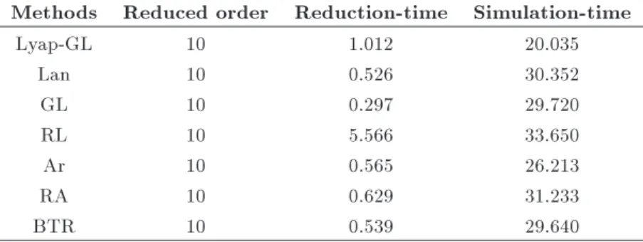
reduction times, and simulation times obtained using 7 methods applied in dierent models is shown in Tables 3 and 4. Table 3 shows the H1 norm error
for each method applied in RC models of orders 30 and 500. Table 4 presents the reduction and simulation times for each method applied in RC model of order 500.
From the results shown in Tables 3 and 4, we conclude that the proposed approach outperforms the competitive one in terms of H1 norm errors. Also, it
performs better with regard to reduction and simula-tion times.
5. Implementation of digital PI controller for higher order systems
To design an eective controller for high order electrical process, we need to reduce the original mathematical model [28]. To do so, we develop an adaptive control strategy whose parameters are taken from reduced system by applying the proposed reduction method, i.e. Lyapunov-Global-Lanczos. In fact, we propose an adaptive digital PI controller applied to large-scale descriptor linear systems.
5.1. PI controller equation
PI controller could be described using the parallel from as shown in Eq. (13) [29,30]:
G(s) = kp+Ksi = u(s)e(s); (13)
where u(s) is a control signal, e(s) is the error between the desired output and the measured one, and kp and
ki are proportional and integral gains, respectively.
In order to implement the PI controller, we determine the Z-Transform of the previous equation.
Table 3. H1 norm errors of each method.
Methods MOR (RC-500) H1 norm error MOR (RC-30) H1 norm error
Lyap-GL 10 0.001 5 0.003
Lan 10 0.003 5 0.533
GL 10 0.033 5 0:946
RL 10 0.030 { {
Ar 10 0.003 { {
RA 10 0.051 { {
BTR 10 0.539 { {
Table 4. Reduction and simulation time of each method. Methods Reduced order Reduction-time Simulation-time
Lyap-GL 10 1.012 20.035
Lan 10 0.526 30.352
GL 10 0.297 29.720
RL 10 5.566 33.650
Ar 10 0:565 26.213
RA 10 0:629 31.233
The result is given in Eq. (19) [28,31]:
U(z) = (kp+1 zki 1)E(z); (14)
where, E(z) = Yc(z) Y (z), with Yc and Y presenting
the desired output and the measured one, respec-tively. As well, we determine the recurrent form of Eq. (19) [32]:
u(k) = u(k 1) + kp(e(k) e(k 1)) + kie(k): (15)
5.2. PI parameters extracted from the reduced system
At rst, we present, in Table 5, the transfer function obtained by the proposed approach as well as 6 bench-mark approaches. From these 7 transfer functions, we conclude that the function obtained by the Lyapunov-Global-Lanczos has a numerator value close to 1; thus, this is the best function to use when calculating the initial parameters of our PI controller.
To calculate the PI parameters, Takahashi method is used in closed loop [33,34]. It is needed to increase the gain of proportional corrector associated with the transfer function obtained by the proposed method in the closed loop until oscillations. Thus, we measure the period oscillation, Tc, corresponding to a
Kc gain.
Figure 10 presents the Takahashi illustration method of setting the PI parameters. The PI param-eters (kp and ki) are determined from the following
relationships [28,35,36]: 8
> < > :
kp = 0:6Kc(1 TTec) kp
Ti =
1:2Kc
Tc
ki=TTei
(16)
in our case, Tc = 2, the sampling period: Te = 1 s,
and Kc= 20:5; thus, we obtain:
kp= 6:15
ki= 2:04 (17)
Figure 11 presents the simulation results of the closed loop step response obtained using the previous param-eters of PI controller applied to the reduced system (order 1) and the original one (order 30). We notice a good correlation between the output trajectories of the reduced system and the original one.
5.3. Adaptive digital PI controller algorithm implemented in Arduino Card
The technical details of the adaptive digital controller PI algorithm implementation in Arduino board are presented in this section.
The adaptation of PI controller is done by the real time adaptation of the kp and kiparameters. We focus
on adding or subtracting a correction term to or from the PI parameters at each iteration based on the real-time error value between the desired output and the measured one until we achieve the best gain according
Figure 11. Closed loop response of the original system and the reduced one obtained with Lyap-GL method.
Figure 10. Takahashi method of setting the PI parameters. Table 5. Reduced transfer functions.
Methods Lyap-GL GL Lanczos Ar RA RL BTR
Transfer functions 0:093
z 0:89 2:27e
16
z 0:67 7:79e
9
z 0:57 9:99e
3
z 0:998 3:33e
3
z 1 4:751e
30
z 1 9:81e
4
to each input. It consists of an error value depending on correction term between the desired output and the measured one at each iteration. The adaptation terms are computed according to the following relationships Eq. (18):
p(k) = e(k 1)=kp(k 1)
i(k) = e(k 1)=ki(k 1) (18)
The new recurrent form of the PI controller is given by:
u(k) =u(k 1) + (kp(k 1) p(k 1))(e(k)
e(k 1))+(ki(k 1)i(k 1))e(k): (19)
As detailed in Table 6, we present the main steps of adaptive digital PI controller algorithm implementa-tion.
5.4. Real-time-implementation
To exhibit the eectiveness and applicability of the pro-posed adaptive PI algorithm, a real-time experiment, composed of real system (order 30), microcontroller
Table 6. Adaptive digital PI controller algorithm. Input: Yc,kp,ki,tol; Output: Ymeasured
(1) Initialization
(a) Initialize the previous control signal: u(k 1) = 0
(b) Initialize the previous error e(k 1) = Yc(k) Ymeasured(k) = 0
(c) Initialize the maximum value of error tol, p, and i
tol = 10 2,
p= 0 and i= 0
(2) Congure of the output pin using PinMode()
(3) Recover and compute the PI gains (kpand ki) in real time
for k=1:1
(a) Congure of input pin using analogRead() (b) Read the measured output Ymeasured
(c) Convert the analog measured value into digital value using the relationship of Analog to Digital Converter (ADC): Digital measured value YDmeasured= (Ymeasured 5)=1023
(d) Compute the error between the desired output Yc and YDmeasured: e(k) = Yc(k) YDmeasured(k)
(e) Adaptation of PI parameters
if (e tol) then kp(k) = kp(k 1) p(k 1), ki(k) = ki(k 1) i(k 1) else if(e tol) then
kp(k) = kp(k 1) + p(k 1), ki(k) = ki(k 1) + i(k 1)
else kp(k) = kp(k 1), ki(k) = ki(k 1) end if
(f) Compute the control signal u using the recurrent PI equation: udigital(k) = u(k 1) + kp(k) (e(k) e(k 1)) + ki(k) e(k 1)
(g) Add a saturation protected condition of the control signal, according to the type of microcontroller
if udigital(k) > delivered voltage by the microcontroller then udigital(k) = delivered voltage by the microcontroller
end if
if udigital(k) < 0 then udigital(k) = 0 end if
(h) Update the previous error and previous control signal: e(k 1) = e(k) and u(k 1) = u(k) (i) Convert the new digital control value into analog control value using the relationships of Digital
to Analog Converter (DAC): u(k)analog= (u(k)digital 255)=5
(j) Transmit the new analog control value to the real system using the analogWrite() (k) Dene a waiting time before moving on to the next iteration
(Arduino UNO) and a computer, has been performed on closed loop.
The Arduino UNO is a microcontroller board based on ATmega328P processor [37]. The board con-tains 6 analog input pins and 14 digital input/output pins of which 6 can be used as Pulse Width Modulation (PWM) outputs (Pin numbers 3, 5, 6, 9, 10, and 11) and provides the 8 bits resolution. In our application, we use pin 10 as analog output and pin 2 as digital input. In order to visualize the output results in real time, we use the PLX-DAQ Spreadsheet tool.
The experimental setups of real system, Arduino UNO and a computer are shown in Figure 12.
Figure 12. Experimental setup.
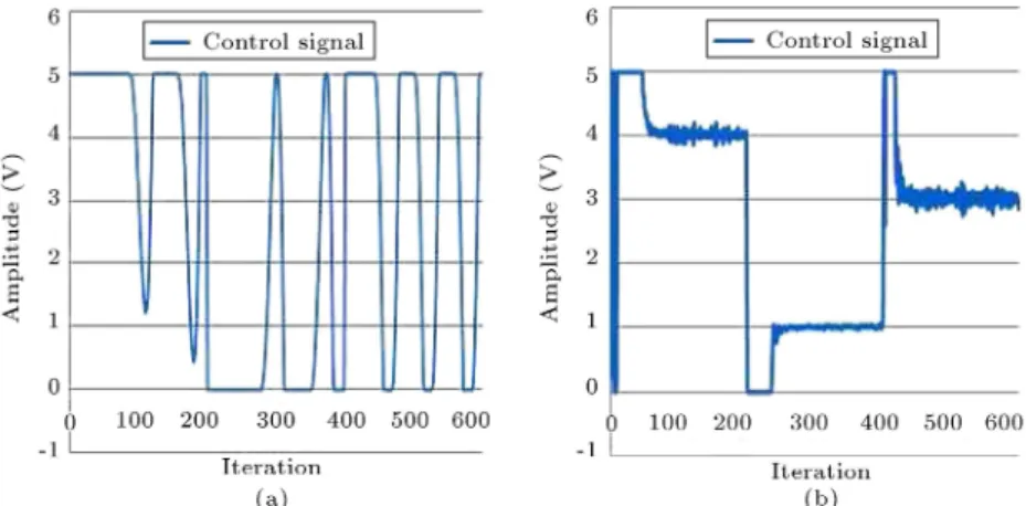
Figure 13(a) and (b) present the output trajecto-ries of real system and input signal, which vary between (4 V, 1 V, 3 V) at each 200 iterations (each iteration is within 0:5 second). We use the xed PI parameters (kp = 6:15 and ki = 2:04) determined by the reduced
system and the adaptive PI parameters, respectively. We notice from Figure 13(a) that the outputs are unstable and the desired outputs are achieved after 100 iterations for inputs equal to 4 V and 1 V, and 50 iterations for an input equal to 3 V, with an error rate between the desired output and the measured one varying between 3% and 15%. However, we see from Figure 13(b) that the outputs are stable and the desired outputs are achieved after 40 iterations for 4 V and 1 V, and 10 iterations for 3 V.
Figure 14(a) and (b) illustrate the control signal obtained by the use of the xed and adaptive PI parameters, respectively. We notice that the control signal obtained by the xed PI controller is unstable; however, it is not the case for the control signal obtained by the proposed adaptive PI controller.
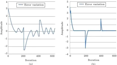
Figure 15(a) and (b) show the error variation obtained between the desired output and the measured one according to the xed PI controller and adaptive one, respectively. We see that the error variation obtained by the adaptive PI parameters is equal to zero,
Figure 13. (a) Closed loop response obtained with xed PI controller. (b) Closed loop response obtained with adaptive PI controller.
Figure 15. (a) Error variation between desired and measured outputs obtained with xed PI controller. (b) Error variation between desired and measured outputs obtained with adaptive PI controller.
Figure 16. Variation of PI controller parameters (Kpand
Ki).
except when changing the input.
Figure 16 shows the variation of the kp and ki
gains according to the error variation between the desired output and the measured one from which we obtained the result illustrated in Figure 13(b).
6. Conclusion
In this paper, we rstly presented the model order reduction method of higher electrical system called Lyapunov-Global-Lanczos, which was based on the Lyapunov and Krylov techniques in generation of projection matrices. Our approach was characterized by minimizing the error between the time responses of the original system and the reduced one as well as H1 error norm preserving the stability of the reduced
system and giving a reduced system of order 1 With the numerator values of their transfer functions very close to 1.
Secondly, we presented an adaptive digital PI controller algorithm that computed the best gains of
PI controller in real time based on the PI controller parameters determined by the reduced system of or-der 1 and the real-time error variation between the desired output and the measured one. Simulation and experimentation results showed eectiveness and robustness of both the proposed algorithms.
References
1. Sinani, K., Gugercin, S., and Beattie, C. \A structure-preserving model reduction algorithm for dynamical systems with nonlinear frequency dependence", IFAC-PapersOnLine, 49(9), pp. 56{61 (2016).
2. Fan, H.Y., Weng, P.C.Y., and Chu, E.K.W. \Numeri-cal solution to generalized Lyapunov/stein and rational riccati equations in stochastic control", Numerical Algorithms, 71(2), pp. 245{272 (2016).
3. Li, T., Weng, C.Y., Chu, E.K.W., and Lin, W.W. \Solving large-scale stein and Lyapunov equations by doubling", Numerical Algorithms, 63(4), pp. 727{752 (2013).
4. Wolf, T. and Panzer, K.H. \The ADI iteration for Lyapunov equations implicitly performs h2 pseudo-optimal model order reduction", International Journal of Control, 89(3), pp. 481{493 (2016).
5. Frangos, M. and Jaimoukha, I. \Adaptive rational interpolation: Arnoldi and Lanczos-like equations", European Journal of Control, 14, pp. 342{354 (2008).
6. Oh, D.C. and Jeung, E.T. \Model reduction for the descriptor systems by linear matrix inequalities", International Journal of Control, Automation and Systems, 8(4), pp. 875{881 (2010).
7. Zhang, Y. and Wong, N. \Compact model order reduction of weakly nonlinear systems by associated transform", International Journal of Circuit Theory and Applications, 29(6), pp. 1{18 (2015).
8. Du, I.P., Vuillemin, P., Vassal, C.P., Briat, C., and Seren, C. \Model reduction for norm approximation:
An application to large-scale time-delay systems", In Delays and Networked Control Systems, 6, pp. 37{55 (2016).
9. Antoulas, A.C., Approximation of Large-Scale Dynam-ical Systems, R.C. Smith, Ed., 1st Ed. pp. 1{508, Advances in Design and Control (2005).
10. Kouki, M., Abbes, M., and Mami, A. \Svd-aora method for dynamic linear time invariant model order reduction", 8th Vienna International Conference on Mathematical Modelling, Vienna, Austria, pp. 695{696 (2015).
11. Nasiri, S.H. and Maghfoori, F.M. \Chebyshev rational functions approximation for model order reduction using harmony search", Scientia Iranica, 20(3), pp. 771{777 (2013).
12. Yuhang, D. and Wu, K.L. \Direct mesh-based model order reduction of PEEC model for quasi-static circuit problems", IEEE Transactions on Microwave Theory and Techniques, 64, pp. 2409{2422 (2016).
13. Aridhi, H., Zaki, H.M., and Tahar, S. \Enhancing model order reduction for nonlinear analog circuit simulation", IEEE Transactions on Very Large Scale Integration (VLSI) Systems, 24(3), pp. 1036{1049 (2016).
14. Xiao, Z.H. and Jiang, Y.L. \Model order reduction of mimo bilinear systems by multi-order arnoldi method", Systems & Control Letters, 94, pp. 1{10 (2016).
15. Jorn, Z. Lei, W., Paul, U., and Rob, R. \A Lanczos model-order reduction technique to eciently simulate electromagnetic wave propagation in dispersive me-dia", Journal of Computational Physics, 315, pp. 348{ 362 (2016).
16. Gugercin, S. \An iterative SVD-Krylov based method for model reduction of large-scale dynamical systems", Linear Algebra and Its Applications, 428, pp. 1964{ 1986 (2008).
17. Malekshahi, E. and Mohammadi, S.M.A. \The model order reduction using LS, RLS and MV estimation methods", International Journal of Control, Automa-tion and Systems, 12(3), pp. 572{581 (2014).
18. Chu, C., Lai, M., and Feng, W. \Mode-order reduc-tions for mimo systems using global Krylov subspace methods", Mathematics and Computers in Simulation, 79, pp. 1153{1164 (2008).
19. Lee, H., Chu, C., and Feng, W. \An adaptive-order rational arnoldi method for model-order reductions of linear time-invariant systems", Linear Algebra and Its Applications, 415, pp. 235{261 (2006).
20. Kouki, M., Abbes, M., and Mami, A. \Arnoldi model reduction for switched linear systems", Int. J. Opera-tional Research, 27(1/2), pp. 85-112 (2016).
21. Barkouki, H., Bentbib, A.H., and Jbilou, K. \An adaptive rational block Lanczos-type algorithm for model reduction of large scale dynamical systems", Journal of Scientic Computing, 67(1), pp. 221{236 (2016).
22. Silvia, G., Enyinda, O., Lothar, R., and Giuseppe, R. \On the Lanczos and Golub{Kahan reduction methods applied to discrete ill-posed problems", Numerical Linear Algebra with Applications, 23(1), pp. 187{204 (2016).
23. Gallivan, K., Grimme, E., and Dooren, P. \A rational Lanczos algorithm for model reduction", Numerical Algorithms, 12, pp. 33{63, 1996.
24. Bonin, T., Fabender, H., Soppa, A., and Zaeh, M. \A fully adaptive rational global arnoldi method for the model-order reduction of second-order mimo systems with proportional damping", Mathematics and Computers in Simulation, 122, pp. 1{19 (2016).
25. Abidi, O. and Jbilou, K. \Balanced truncation-rational Krylov methods for model reduction in large scale dy-namical systems," Computational and Applied Mathe-matics, 35, pp. 1{16 (2016).
26. Meiling, W.J., Chu, C., Yu, Q., and Kuh, S.E. \On projection-based algorithms for model-order reduction of interconnects", IEEE Transactions on Circuits and Systems I: Fundamental Theory and Applications, 49(11), pp. 1563{1585 (2002).
27. Kouki, K., Abbes, M., and Mami, A. \Arnoldi model reduction for switched linear systems", The 5th In-ternational Conference on Modeling, Simulation and Applied Optimization, Hammamet, Tunisia, pp. 1{6 (2013).
28. Malwatkara, G., Sonawaneb, S., and Waghmarec, L. \Tuning PID controllers for higher-order oscillatory systems with improved performance", Automatica, 48, pp. 347-353 (2009).
29. Alexander, S.A. and Thathan, M. \Design and devel-opment of digital control strategy for solar photovoltaic inverter to improve power quality", Journal of Control Engineering and Applied Information, 16(4), pp. 20-29 (2014).
30. Rebai, A., Guesmi, K., and Hemici, B. \Design of an optimized fractional order fuzzy PID controller for a piezoelectric actuator", Journal of Control Engineer-ing and Applied Information, 17(3), pp. 41-49 (2015).
31. Isakssona, A.J. and Graebe, S.F. \Analytical PID parameter expressions for higher order systems", Au-tomatica, 35, pp. 1121-1130 (1999).
32. Malwatkar, G.M., Khandekar, A.A., and Nikam, S.D. \Pid controllers for higher order systems based on maximum sensitivity function", 3th International Con-ference on Electronics Computer Technology (ICECT), Kanyakumari, India, pp. 259{263 (2011).
33. Franklin, G.F., Powell, J.D., and Workman, M.L., Digital Control of Dynamic Systems, Addison and Wesley (1990).
34. Kovacic, Z. and Bogdan, S., Fuzzy Controller Design: Theory and Applications, 19, CRC press (2005).
35. Gharib, M. and Moavenian, M. \Synthesis of robust PID controller for controlling a single input single output system using quantitative feedback theory tech-nique", Scientia Iranica. Transaction B, Mechanical Engineering, 21(6), pp. 1861{1869 (2014).
36. Hasankola, M.D., Ehsaniseresht, A., Moghaddam, M., and Saba, A. \Analysis, modeling, manufacturing and control of an elastic actuator for rehabilitation robots", Scientia Iranica. Transaction B, Mechanical Engineering, 22(5), pp. 1855{1865 (2015).
37. Massimo, B. and David, C. \Arduino" (2016). [Online]. Available: https://www.arduino.cc
Biographies
Mohamed Kouki was born in 1986 in Tunisia. He received his MSc degree from the University of Tunis ELmanar at the Faculty of Sciences of Tunis in 2011. He received his PhD degree in Electrical Engineering
from the Faculty of Sciences of Tunis in 2014. His main research interests include order reduction methods and control algorithms in microelectronics.
Mehdi Abbes was born in 1978 in France. He received the BSc degree in Electronics and Instru-mentation, in 2001, from the High School of Sciences and Techniques of Tunis. In 2004, he obtained the MSc degree in measurement and instrumentation at the High Institute of Applied Sciences and Technology of Tunis. He received his PhD degree in Electrical Engineering from the National School of Engineering of Tunis, in 2009. His main research interests include bond graph modeling of thermouid systems, reduction order methods for large scale systems, control algo-rithms in microelectronics.
Abdelkader Mami was born in Tunisia. He is a Professor in Faculty of Sciences of Tunis. He received his Dissertation H.D.R (Enabling to Direct of Research) from the University of Lille (France) in 2003; he is a member of Advice Scientic in Faculty of Science of Tunis. He is a President of commutated thesis of electronics in the Faculty of Sciences of Tunis.
![Figure 10 presents the Takahashi illustration method of setting the PI parameters. The PI param-eters (k p and k i ) are determined from the following relationships [28,35,36]: 8 > < > : k p = 0:6K c (1 T T ec )kpTi=1:2KTcc k i = T T e i (16)](https://thumb-us.123doks.com/thumbv2/123dok_us/8374943.2224515/8.892.484.826.572.798/figure-presents-takahashi-illustration-parameters-determined-following-relationships.webp)