ABSTRACT
I
n this paper we study the face poset, and a random walk on the regions of the Braid arrangement as a special case when n = 4. The transition matrix for Braid arrangement considered one of the most important findings in this research. In addition to this, we will calculate the face poset, the stationary distribution and the eigenvalues of transition matrix for Braid arrangement.Key word: Braid arrangement, face, chamber, random walk, transition matrix, stationary distribution.
1. INTRODUCTION
An arrangement of hyperplanes is a finite collection of codimension one subspace in a finite dimensional vector space over R(ℂ). Let L = L(𝒜𝒜) be the intersection poset of 𝒜𝒜. L is the set of non-empty intersections of hyperplanes in 𝒜𝒜 ordered by reverse inclusion. By convention L includes V as its unique minimal element. The intersection of the form x = ⋂H∈𝒜𝒜HσH is called a face of 𝒜𝒜, where σH ∈ {+, −, 0} and H0
= H. The sign vector of x is the sequence σ(x) = (σH)H∈𝒜𝒜. A face c is called chamber if σH(c) ≠0 for all H ∈ 𝒜𝒜. The set of faces of 𝒜𝒜 is called the face poset of 𝒜𝒜 which is denoted byℱ. The face poset is partially ordered by:
x ≤ y ⟺ for each H ∈ 𝒜𝒜 either σH(x) = 0 or σH(x) = σH(y).
Let J = {+, −, 0}. We may view each face F ∈ℱ(A) as a map F:{1, . . . , n} → J defined by F(k) = signαH(p) for any p ∈ F. Note that F(k) = 0 if and only if F ⊆HK, and if F(k) ≠ 0, then the sign indicates whether F is in the positive or negative half-space determined by HK. Which side is called positive depends on the original choice of αK. Let W = Jn, and let πH: W → J be the projection onto the k-th coordinate. Define a map σ:ℱ→W by:
πKσ(F) = �
+ if F(K) > 0 0 if F(K) = 0
− if F(K) < 0
Note that the choice of which half-space to label + or − is arbitrary, but fixed, for more details see [1][2][3][4].
2. THE FACE POSET OF BRAID ARRANGEMENT
The Braid arrangement in Rn consist of �n
2� hyperplanes Hij = {(x1, …,xn): xi = xj} (i < j). The chambers are
associated with a common ordering of the coordinates and so with one of the n! permutations. When n= 4, for example, one of the 24 chambers is the region defined by x1 > x4 > x2 > x3, corresponding to the partition 1423. The hyperplane
Hij intersect in the line x1 = … = xn. The Braid arrangement therefore give rise to an arrangement in (n-1)-dimensional
space When n = 4, the resulting arrangement of 6 planes in R3 may be pictured as in Figure (1). The great circle
corresponding to Hij is labeled i-j. (The equator is not one of the great circles of the arrangement).Each chamber is labeled with the associated permutation.
Corresponding Author: Mohammed K. Ali*
2,
1,2Al-Mustansiriyah University,
Rabeaa G. Al-Aleyawee, Mohammed K. Ali* / Random Walks and Braid Arrangement / IJMA- 7(2), Feb.-2016.
Fig.1: The Braid arrangement when n = 4
The faces of a chamber C are obtained by changing to equalities some of the inequalities defining C. For example, the chamber x2> x3> x1> x4 has a face given by x2> x3> x1 = x4, which is also a face of the chamber x2> x3> x4> x1.
This common face is represented by edge between 2314 and 2341 in Figure (1).Similarly, the vertex labeled 2 in the figure corresponds to the face x2> x1 = x3 = x4; it is a face of six chambers, corresponding to the six possible orderings
of the indices 1, 3, 4.
It is useful to encode the system of equalities and inequalities defining a face F by an ordered partition (B1, …, BK) of
{1, …, n}. Here B1, …, BK are disjoint nonempty sets whose union is {1, …, n}; they are called the blocks of the
partition, and their order counts. For example, the face x2> x3> x1 = x4 corresponds to the 3-block ordered partition
({2},{3}, {1, 4}), and the face x2> x1 = x3 = x4 corresponds to the 2-block ordered partition ({2}, {1, 3, 4}). Notice
that there is also a (unique) 1-block ordered partition, corresponding to the face x1 = x2 = x3 = x4. When we pass from
R4 to a 3-dimensional quotient to make the hyperplanes have trivial intersection, this face becomes {0}. It does not show up in Figure (1) because its intersection with the sphere is empty [5][10].
Theorem 2.1 [6]: There is an order-isomorphism ∅2: L(𝒜𝒜n) →∏n between the intersection lattice L(𝒜𝒜n) for the Braid
arrangement 𝒜𝒜n and the set partition lattice ∏n.
Fig. 2: Hasse diagram between the intersection lattice for the Braid arrangement and the set partition lattice
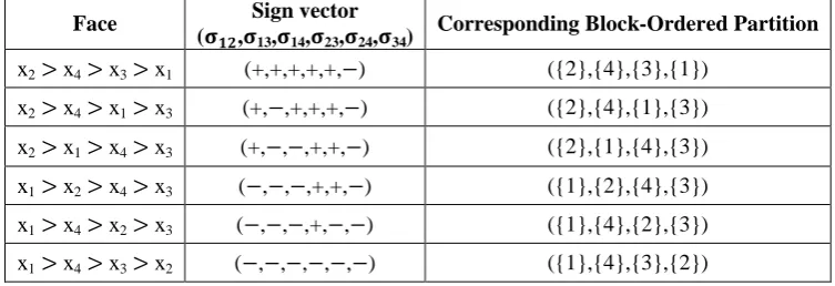
Example 2.2: In 𝒜𝒜4 Braid arrangement, the sign vectors for each face are given in the following Table.
Face Sign vector
(𝛔𝛔𝟏𝟏𝟏𝟏,𝛔𝛔13,𝛔𝛔14,𝛔𝛔23,𝛔𝛔24,𝛔𝛔34)
Corresponding Block-Ordered Partition
x2> x4> x3> x1 (+,+,+,+,+,−) ({2},{4},{3},{1})
x2> x4> x1> x3 (+,−,+,+,+,−) ({2},{4},{1},{3})
x2> x1> x4> x3 (+,−,−,+,+,−) ({2},{1},{4},{3})
x1> x2> x4> x3 (−,−,−,+,+,−) ({1},{2},{4},{3})
x1> x4> x2> x3 (−,−,−,+,−,−) ({1},{4},{2},{3})
x1> x4> x3> x2 (−,−,−,−,−,−) ({1},{4},{3},{2})
1/2/3
123
13/2
12/3
x
1=x
2=x
3V=
0
�
x
2=x
3x2> x3> x4> x1 (+,+,−,+,+,+) ({2},{3},{1},{4})
x2> x1> x3> x4 (+,−,−,+,+,+) ({2},{1},{3},{4})
x4> x3> x2> x1 (+,+,+,−,−,−) ({4},{3},{2},{1})
x4> x2> x3> x1 (+,+,+,+,−,−) ({4},{2},{3},{1})
x4> x2> x1> x3 (+,−,+,+,−,−) ({4},{2},{1},{3})
x4> x1> x2> x3 (−,−,+,+,−,−) ({4},{1},{2},{3})
x1> x4> x3> x2 (−,−,+,−,−,−) ({1},{4},{3},{2})
x4> x3> x1> x2 (−,+,+,−,−,−) ({4},{3},{1},{2})
Table-1: Face, sign vectors, and corresponding block-ordered partition for 𝒜𝒜4 arrangement
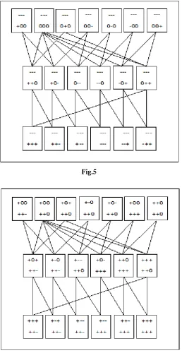
The poset of the Braid arrangement when n = 4 will be large so much, So we will partition it as follows: 1. Figure (5), shows the poset that obtained from H23∩H24∩H34 in the northern hemisphere.
2. Figure (6), shows the poset that obtained from H13∩H14∩H34 in the northern hemisphere.
3. Figure (7), shows the poset that obtained from H12∩H14∩H24 in the northern hemisphere.
4. Figure (8), shows the poset that obtained from H12∩H13∩H23 in the northern hemisphere.
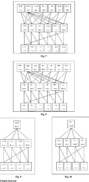
5. Figure (9), shows the poset that obtained from H23∩H14 in the northern hemisphere.
6. Figure (10), shows the poset that obtained from H12∩H34 in the northern hemisphere.
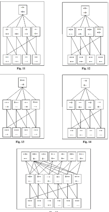
7. Figure (11), shows the poset that obtained from H13∩H24 in the northern hemisphere.
Fig.3: The northern hemisphere of 𝒜𝒜4 Braid arrangement
8. Figure (12), shows the poset that obtained from H13∩H24 in the southern hemisphere.
9. Figure (13), shows the poset that obtained from H12∩H34 in the southern hemisphere.
10. Figure (14), show the poset that obtained from H23∩H14 in the southern hemisphere.
11. Figure (15), shows the poset that obtained from H12∩H13∩H23 in the southern hemisphere.
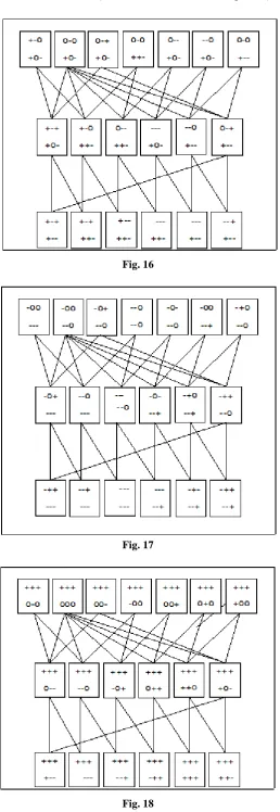
12. Figure (16), shows the poset that obtained from H12∩H14∩H24 in the southern hemisphere.
13. Figure (17), shows the poset that obtained from H13∩H14∩H34 in the northern hemisphere.
Rabeaa G. Al-Aleyawee, Mohammed K. Ali* / Random Walks and Braid Arrangement / IJMA- 7(2), Feb.-2016.
Fig. 4: The southern hemisphere of 𝒜𝒜4 Braid arrangements
Fig.5
Fig. 7
Fig. 8
Rabeaa G. Al-Aleyawee, Mohammed K. Ali* / Random Walks and Braid Arrangement / IJMA- 7(2), Feb.-2016.
Fig. 11 Fig. 12
Fig. 13 Fig. 14
Fig. 16
Fig. 17
Rabeaa G. Al-Aleyawee, Mohammed K. Ali* / Random Walks and Braid Arrangement / IJMA- 7(2), Feb.-2016.
3. THE TRANSITION MATRIX K
In [7] Brown found the transition matrix for a subset of Braid arrangement when n = 4, so we will find the transition matrix for all the regions of Braid arrangement.
3.1. A random walk on the regions [8],
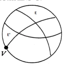
Bidigare, Hanlon, and Rockmore in [9] used the projection operators to define the following walk on the regions: If the
walk is in region E, choose a vertex v at random and move to the projection E′ = vE. This walk is described
mathematically by its transition matrix K. The rows and columns of K are indexed by the regions, with K(E, E′) being the chance of moving from to E′in one step. Thus
K(E, E′) = 1/a0Λ(E, E'),
Where Λ(E, E') is the number of vertices v of E′such that vE = E′.
Fig. 19: The projection of E on v
3.2.The transition matrix of Braid arrangement
We should now be able to construct geometrically the transition matrix involving all the regions. For example, starting with the region 1234, you choose at random a proper subset of the places and put those first in the original order. So if you choose places 1 and 3, then you put those first and get 1324. Choosing 1 or 12 or 123 will all lead to 1234 again, so the probability of moving 1234 ⟹ 1234 is 3/14. So choosing subset S leads to permutation pi as follows:
S 1 2 3 4 12 13 14 23 24 34 123 124 134 234
pi 1234 2134 3124 4123 1234 1324 1423 2314 2413 3412 1234 1243 1342 2341
So the probability of moving 1234 ⇒ pi is, for example, 1234 ⇒ 1234 3/14
1234 ⇒ 4321 0 1234 ⇒ 3412 1/14 1234 ⇒ 2314 1/14 1234 ⇒ 4312 0
and so forth. Really, what is happening here is the probability of 1234 ⇒ pi is 3/14 if pi has 0 descents, 1/14 if pi has 1 descent, 0 if pi has 2 or 3 descents. Therefore the following matrix is the transition matrix of all regions for Braid arrangement when n = 4.
2431 2413 2143 1243 1423 1432 1342 3142 3412 3421 3241 2341
2431 3 1 1 1 0 0 0 0 0 0 1 1
2413 1 3 1 1 0 0 0 0 0 0 1 1
2143 1 1 3 1 1 1 0 0 0 0 0 0
1243 1 1 1 3 1 1 0 0 0 0 0 0
1423 0 0 1 1 3 1 1 1 0 0 0 0
1432 0 0 1 1 1 3 1 1 0 0 0 0
1342 0 0 0 0 1 1 3 1 1 1 0 0
3142 0 0 0 0 1 1 1 3 1 1 0 0
4123 0 1 0 1 1 0 0 0 1 0 0 1
4213 0 1 1 0 1 0 1 0 0 1 0 0
4231 1 0 0 0 1 0 0 1 0 1 0 1
4321 1 0 1 0 0 1 0 0 0 1 1 0
4312 1 0 0 1 0 1 0 1 1 0 0 0
Table-2: The transition matrix for all regions of Brid arrangement
3.3. The eigenvalues of transition matrix for Braid arrangement
The intersection for the Braid arrangement with the sphere S2 is empty. Therefore the Braid arrangement cannot
consider as a sphere, and hence the eigenvalues for the transition matrix when n = 4 cannot be calculated using the account eigenvalues laws as in [10].So the following eigenvalues are found by using Matlab program.
13.0409, 5.9191, 0.0961, 0.9440, 6.1623, 6.1623, 6.1623, 1.0000, 1.0000, 1.0000, 1.0000, 6.1623, 6.1623, -0.1623, -0.1623, 3.0000, 3.0000, 3.0000, 3.0000, 3.0000, 3.0000, -0.1623, -0.1623, -0.1623
2314 3214 3124 1324 1234 2134 4132 4123 4213 4231 4321 4312
1 0 1 0 0 0 0 0 0 1 1 1
0 0 0 1 0 1 1 1 1 0 0 0
1 1 0 0 0 1 0 0 1 0 1 0
0 0 1 0 1 0 0 1 1 1 0 0
1 0 0 0 1 0 0 1 1 1 0 0
0 1 0 1 0 0 1 0 0 0 1 1
0 0 0 1 1 1 1 0 1 0 0 0
1 1 1 0 0 0 0 0 0 1 0 1
0 0 1 0 1 0 1 1 0 0 0 1
0 1 0 0 0 1 0 0 1 1 1 0
0 1 1 1 0 0 1 0 0 0 1 0
1 0 0 0 1 1 0 1 0 1 0 0
3 1 1 0 1 1 0 0 0 1 0 0
1 3 1 1 0 1 0 0 0 0 1 0
1 1 3 1 1 0 0 0 0 0 0 1
0 1 1 3 1 1 1 0 0 0 0 0
1 0 1 1 3 1 0 1 0 0 0 0
1 1 0 1 1 3 0 0 1 0 0 0
0 0 0 1 0 0 3 1 1 0 1 1
0 0 0 0 1 0 1 3 1 1 0 1
0 0 0 0 0 1 1 1 3 1 1 0
1 0 0 0 0 0 0 1 1 3 1 1
0 1 0 0 0 0 1 0 1 1 3 1
Rabeaa G. Al-Aleyawee, Mohammed K. Ali* / Random Walks and Braid Arrangement / IJMA- 7(2), Feb.-2016.
4. THE STATIONARY DISTRIBUTION ON THE REGIONS
Definition 4.1 [11]: Let P = 𝒫𝒫ij be the transition matrix, then the vector π is called stationary distribution for P if
∀ j ∈ W⊂N (the set of natural number) it satisfies: 0 ≤πj≤ 1.
∑j ∈ Wπj = 1.
πj = ∑i∈Wπi𝒫𝒫ij.
This equation in matrix notation is π = π P, where π = (πi: i ∈ W) is a row vector.
One way to compute the stationary distribution for P is to solve the linear equations π.P = P.
For example, let P =�
6/10 1/10 3/10 1/10 7/10 2/10 2/10 2/10 6/10�
, since we know that π.P = P,
We can write this as a series of equations: 6/10π1 + 1/10π2 + 2/10 π3 = π1
1/10 π1 + 7/10 π2 + 2/10 π3 = π2
π1 + π2 + π3 = 1.
Now by solving these equations we get that π≈(0.2759, 0.3448, 0.3793).
In case the random walk on regions the stationary distribution π of the region N represents the chance that the random walk is in E after a large number of steps from any starting region E′.
4.2. The stationary distribution of Braid arrangement
The confusion we are having is due to the fact that in Figure (1), the equator (dotted circle) is not a plane in the braid arrangement, so the regions touching the equator all continue on the bottom (for example the rest of the region labeled 3421 (on the bottom) is antipodal to 1243 on the top. (The entire picture on the bottom is antipodal to the one on the top, so there are 24 complete triangular regions in all).Thus all regions are bounded by 3 sides and so the stationary distribution is uniform (probability=1/24 for each region). This follows from(proposition.1,[8]).
REFERENCES
1. Orlik, P. and Terao, H., “Arrangements Of Hyperplanes”, Grundlehren Math. Wiss., vol. 300, Springer-Verlag
Berlin, (1992).
2. Stanly, R. P., "An Introduction To Hyperplane Arrangement", IAS/Park City Mathematics Series, V. 14, 2004. 3. Orlik, P., "Introduction To Arrangements", CBMS Lecture Notes 72, Amer. Math. soc, (1989).
4. Saliola, F.V., "The Face Semigroup Of a Hyperplane Arrangement", Canad. J. Math. Vol. 61 (4), 2009
pp.904-929.
5. Saliola, F.V., "On The Quiver Of Descent Algebra", J. Algebra 320(2009).
6. Al-Ta'ai, A. H. and Al-Aleyawee, R. G., "The hypersolvable and free arrangements", A Ph.D. Thesis
Submitted to College of Science-University of Al-Mustansiriyah, 2005.
7. Brown, K. S., "Semigroups, rings, and Markov chains". J. Theoret. Probab., 13(3):871–938, (2000).
8. Diaconis, P., Billera, L.J., Brwon, K.B., "Random walks and plane arrangements in three dimensions", Math. Monthly 106 (1999), no. 6, 502-524.
9. Bidigare, P., Hanlon, P, and Rockmore, D., "A combinatorial description of the spectrum for the Tsetlin
library and its generalization to hyperplane arrangements", Duke Math. J., to appear, Vol. 99, No. 1, (1999).
10. Brown, K. S., and Diaconis, P., "Random walks and hyperplane arrangements" Ann. Probab., 26(4):1813–
1854, (1998).
11. Serfozo, R., “Basics of Applied Stochastic Processes, Probability and its Applications”. Springer-Verlag
Berlin Heidelberg 2009.
Source of support: Nil, Conflict of interest: None Declared
[Copy right © 2016. This is an Open Access article distributed under the terms of the International Journal of Mathematical Archive (IJMA), which permits unrestricted use, distribution, and reproduction in any