Available online throug
ISSN 2229 – 5046
FUZZY OPTIMAL PRODUCTION INVENTORY CONTROL
BAYOUMI. M.ALI HASSAN*, EL-ALAOUI T. M**.
*Faculty of Computer and Information, Cairo University.
**Dept. of Mathematics, Faculty of Science, Girl’s Branch, El-Azhar University.
(Received On: 24-06-15; Revised & Accepted On: 19-05-17)
ABSTRACT
I
n this paper, a fuzzy optimal multi-level production–inventory control model is formulated as optimal control problem in a decentralized supply chain having individual decision makers (DMs) where each facility is controlled independently in a continuous review. The adopted approach is the Triangular Fuzzy Numbers (TFNs) utilization. Accordingly, the genetic algorithm is developed, coded with C++ Programming language. Numerical example and sensitivity analysis are discussed to illustrate the optimal decision in fuzzy environments. This paper introduce a method so that the production rate that the manufacturer should hold along the chain such that the resources of each company are used the best and the inventory overall cost is to be minimized?Key words: Fuzzy Optimal control; supply chain management (SCM); Chebyshev Approximation; Genetic Algorithm.
1. INTRODUCTION
In most of the existing inventory models, it is assumed that the inventory parameters, objective goals are deterministic and fixed. But, if we think of their practical meaning, they are uncertain. The fuzzy criterion models are just able to incorporate the expert knowledge via fuzzy membership functions. So, fuzzy criterion models are closer to the spirit of modern decision-making, thinking ( see Turban 1998) , than the existing inventory models. In view of the fuzziness of goals, constraints and actions in real-world, decision making problems such as inventory control systems and service facility systems, metaheuristic algorithms (see Thangavel 2005) and fuzzy dynamic programming have been widely applied. In 1870, Bellman and Zadeh considered the classical decision model and suggested several models for decision making in a fuzzy environment. Bellman .R.E. and L.A.Zadeh (see Bellman 1970 and Zimmermann 1985) deal with the application of fuzzy set theory in mathematical programming. (See Kacprzyk 1983, Esogbue and Bellman 1984 and Zimmerman 1983, 1991 and 2000) reviewed development and applications in the field of fuzzy inventory control.
In this paper, the imprecision and uncertainty are described in three cases:
A. When production costs are presented as Triangular Fuzzy Numbers (TFNs). B. When holding costs are presented as Triangular Fuzzy Numbers (TFNs). C. When set-up costs are presented as Triangular Fuzzy Numbers (TFNs). Throughout the supply chain described by linguistic terms.
2. MODEL DESCRIPTION
Assumptions and Notations
For the Nth (N =1, 2,…, n1) item, it is assumed that:
(i) Initial stock and demands are known. (ii) Demand is continuous and deterministic. (iii)Production is continuous and deterministic. (iv)Inventory level is continuous and deterministic. (v) Deterioration rate is known and deterministic. (vi)Backlog or shortage is not considered.
Corresponding Author:
Bayoumi. M.Ali Hassan*,
For the Nth (N=1, 2,…,n1) item :
DN(t) = D0(t)+D1N (t): demand rate at time t where D0N , D1PN are known.
Pn(t) =
0
. ( )
m
K kN k P T t
=
∑
: Production rate at time t,where P0N, P1N,…,PmN are known and TK(t) is the Kth Chebyshev polynomial .
IiN(t) :inventory level at time t in the ith cycle.
pN
C
~
: Fuzzy production cost per unit item and time represented as TFN.N
h
~
: Fuzzy holding cost per unit item and time represented as TFN. aN : Storage area for the Nth
item.
p
S
~
: Fuzzy set up time per echelon represented as TFN.[ti-1,ti] : the interval of the ith cycle, where i= 1,2,…,ℓ.
ζѕ : is the Chebyshev points in the interval [-1,1] , where ѕ = 0, 1, 2,…,j. where:
ℓ Level number.
T Time length of each level. n1 number of items.
Μ maximum space available for storage BT Total budget.
Defuzzification of parameters
The triangular fuzzy number TFN is computed using the equation (A).
1 2 3
ˆ
2
4
A
=
a
+
a
+
a
(A)where
A = (a1, a2, a3) is a TFN.
Parameter 1:
C
~
pN is a Fuzzy production cost per unit item and unit time represented as TFNParameter 2:
h
~
N is a fuzzy holding cost per unit item and unit time represented as TFNParameter 3:
S
~
p is a fuzzyset up time per cycle represented as TFN.Fuzzy parameters TFN Defuzzification
pN
C
~ (c1, c2, c3)pN
C
=4 2 2 3 1 c c
c + +
N
h
~
(h1 , h2, h3) hN =4
2 2 3
1 h h
h + +
p
S~ (s1, s2, s3) Sp =
4 2 2 3
1 s s
s + +
Table-1: Defuzzification of Parameters
Mathematical formulation:
This is a serial decentralized supply chain system with individual decision makers (DMs) where each facility is controlled independently in a continuous review.
The overall SC inventory control is achieved at two levels consisting of Producers or manufacturers, a central warehouse and distributors or retailers. (Figure 1)
Figure-1: Serial supply chain system
Warehouse
Each one of them holds inventory in some form to support the requirement at the end of the supply chain. This problem is formulated as an Optimal Control Problem.
We assume that the system is multi-item production with dynamic demands. Here, the items are produced at a variable rate and deteriorate at a constant rate. Demands for the items are time dependent and the stock level at time t decreases due to deterioration and consumption. Shortages are not allowed.
The imprecision and uncertainty are described in three cases:
a. When production costs are presented as Triangular Fuzzy Numbers (TFNs). b. When holding costs are presented as Triangular Fuzzy Numbers (TFNs). c. When set-up costs are presented as Triangular Fuzzy Numbers (TFNs).
The differential equation for items representing the above system during a fixed time-horizon, T, are given by:
Min J = N pN N p
n
N n
i
N
I
t
C
P
t
dt
ns
h
+
+
∫ ∑
= =)]
(
)
(
[
1 1 1 (1.a)= iN p
n p n i i t ip t N N pN n N n i iN t i t iN
N
I
t
C
P
t
dt
h
P
t
dt
ns
h
+
+
∑∑ ∫
+
∑∑ ∫
= = = = −)
(
)]
(
)
(
[
11 1 1 1 1 1 1 1 (1.b) Subject to
dt
t
dI
iN(
)
= PN(t) – DN(t) – θN IiN (t), ti-1 ≤ t ≤ tiN1 (2.a)
dt
t
dI
iN(
)
= – DN(t) – θN IiN (t), tiN1≤ t ≤ ti (2.b)
Μ
≤
∑
= N n NiN
t
a
I
(
)
1 1 (3) T p N n i iN t i t pN n p
ns
dt
t
P
C
+
≤
Β
∑
∑
∫
= = −)
(
1 1 1 1 1 (4) andJ1 =
h
I
t
C
pNP
Nt
dt
n N n i t i t iN
N
(
)
(
)]
[
1 1 1 1 1+
∑ ∑ ∫
= = −and J2 =
h
P
iNt
dt
n p n i i t ip t
N
(
)
1
1 1 1
∑ ∑ ∫
= =(5)
With the initial and boundary conditions: DN (t) = D0N+D1N t
IiN(ti) = IiN (ti-1) = 0 and
ti = iT/n where i = 1, 2,…,n1 (6)
The problem can be converted from the t- interval [ti-1, tip1] into the ζ –interval [0, 1], via the transformation
ζ = 1 1 1 − −
−
−
i iN it
t
t
t
(B)So, equation (8) is reduced to:
J1 =
t
t
h
NI
iNξ
C
pNP
Nξ
d
ξ
n
N n
i
i
iN
)
[
(
)
(
)]
(
1 0 1 1 1 1 1+
−
∫
∑∑
− − − (7) andξ
ξ
d
dI
iN(
)
= (tip1- ti-1) (up (ξ) – D0N – D1N ((t iN1-t i-1 ) ξ + ti-1 ) – θN I iN (ξ) (8)
Where
IiN (0) = 0 and
P
N(
ξ
)
=(
)
Assume
ξ
ξ
d
dI
iN(
)
= ΦiN(ξ) (10)
IiN (ξ s) =
(
)
0 j iN N j sj
b
Φ
ξ
∑
=
(11)
Where bsj are the elements of the matrix as given in (El gendi 1969) method:
1 cos
k sj j os
b
k
π
=
= −
∑
, s = 0, 1,…,k and i = 1, 2…,nHere: P00, P01,…,Pmn1 are unknown constants and Tk(ξ), k = 0, 1, 2…,m is the k th
Chebyshev polynomial .
Using equations (9, 10, 11), the system of constraints (8), can be written in the following form
ΦiN(ξ s) = (t iN1-t i-1 ) (
(
)
0
ξ
k m k kNT
P
∑
=– D0N – D1N ((t iN1-t i-1 ) ξ s + ti-1 ) – θN
(
)
0 j iN N j sj
b
Φ
ξ
∑
=(12)
and ξ s = ½
1 cos
s
k
π
−
s = 0,1,…,k (13)Equation (7) can be approximated using El-Hawary technique (see El-Gindy and El-Hawary 1995) and substituting from (9,10,11, 12) into (7) we get:
J1(P00,P01,…,Pmn1) =
(
1)
1 1 1 1 n n N i i N it
t
= = −−
∑∑
0 0 0
(
( )
(
(
)))
k k m
kj N js iN s pN kN k j
j s k
b h
b
ξ
C
P T
ξ
= = =
Φ
+
∑
∑
∑
(14)Integrating (2.b) and the 2nd part of (5) using (7) we get
IiN (t) = D0N (exp (θN (ti-t)) -1) / θN +D1N (ti exp (θN (ti-t)) -t ) / θN
- D1N (exp (θN (ti-t)) -1 ) / θ2N t iN1≤ t ≤ t i (15)
J2 = N i iN N N i iN N
n
i N
n
N
N
D
t
t
D
t
t
h
[
(exp(
θ
(
1))
1
)
/
θ
2 0(
1)
/
θ
1 0 1 1
−
−
−
−
∑
= =∑
– D1N (ti 2- ti N12) / 2θN 2 – ( D1N exp θN (ti - tiN1) -1) / θN 3
+ D1N (ti - ti N1) / θN 2 + D1N (ti exp θN ( ti - tiN1) -ti) / θN 2 ] (16)
To find the values of tiN1, equating equations (13) and (17), we get:
D0N(exp (θN (ti-t)) -1) / θN + D1N(ti exp (θN (ti-t)) -t )/θN
- D1N (exp (θN (ti-t)) -1) / θ2N =
(
)
0 j iN N j kj
b
Φ
ξ
∑
=, i=1, 2,...,n, N= 1, 2,…,n1 (17)
Then the above optimization problem can be written in the following form:
Min J = J1 + J2 +n S p (18)
Subject to
∑
= 1 1 n N[ (t iN1-t i-1 ) (
(
))
0 0 j k m k kN k j
kj
P
T
b
∑
ξ
∑
= =
] ≤ M (19)
(
)
1
1 1 1
0 0
1
(
)
n n k m
kj kN k j
N i j k
iN i pN p
t
t
b
P
T
ξ
C
ns
= = − = =
∑∑
−
∑ ∑
+
≤ BT (20)This is a nonlinear programming problem (NLPP) of the performance with a system of constraints, and we solve it using the Genetic algorithm (GA).
This is a fuzzy Non-Linear optimization problem of the performance index subject to some constraints.
a. Fuzzy production cost
( )
C
pN :The values of the production cost parameter C for our algorithm can be determined from the production engineer experiences to be as follows:
C1 =8, C2=10 and C3=15
C
~
pN
= (8, 10, 15) is a TFN.So,
C
pN
=4 2 2 3
1
c
c
c
+ + (A)To defuzzify our model we must substitute the fuzzy value of the production cost by its crisp value using equation (A)
b. Fuzzy holding cost
( )
h
N :The values of the cost parameter C for our algorithm can be determined from the finance manger experiences or the person which has the responsibility of inventory to be as follows:
C1 = 7, C2 = 8 and C3= 12 and so
C
~
pN= (7, 8, 12) is a TFNSo,
h
N
=4 2 2 3
1
c
c
c
+ + (A)To defuzzify our model we must substitute the fuzzy value of the holding cost by its crisp value using equation (A), so
N
h
= 8.75 units.c. Fuzzy setup cost
( )
p S
The values of the set up cost C for our algorithm can be determined from the finance manger experiences to be as follows:
C1 =5, C2= 6 and C3= 9
pN
S
~
= (5, 6, 9) is a TFNN
p
S
=4 2 2 3
1
c
c
c
+ + (A)To defuzzify our model we must substitute the fuzzy value of the setup cost by its crisp value using equation (A), so
N p
S
= 6.5 unitsNow the reduced Non-Linear constrained optimization problem can be solved
Using a Genetic algorithm (GA).
3. GENETIC ALGORITHM
A genetic algorithm (GA) is a heuristic search process for optimization that resembles natural selection. The GA was first proposed by Holland. It has been applied successfully in different areas.
Genetic Algorithms are a class of optimization algorithms based on “survival of the fittest”. The basic idea is that each possible solution is a member of a population, and any given population is keeping track of multiple solutions. When going through a genetic algorithm a good solution is more likely to survive and hence more likely to reproduce.
Parents in a genetic algorithm are selected at random from the available population, and the new trial solutions (children) are created from the parents. When these children are added to the population, they occasionally have mutations which add more variety to the population.
Genetic programming operators
The four general genetic operators are: crossover, reproduction, mutation, and inversion. The following overview describes each in brief.
Crossover, considered along with reproduction, to be the two foremost genetic operations. It is mainly responsible for the genetic diversity in the population of programs. Similar to its performance under genetic algorithms, crossover operates on two programs (a binary operator), and produces two child programs. Two random nodes are selected from within each program and then the resultant ``sub-trees'' are swapped, generating two new programs. These new programs become part of the next generation of programs to be evaluated.
Reproduction, the second main operation, is performed by simply copying a selected member from the current generation to the next generation.
In genetic programming, when an individual incestuously mates with itself (or copies of itself), the two resulting offspring will, in general, be different as before, the Darwinian reproduction operation creates a tendency toward convergence; however, in genetic programming, the crossover operation exerts a counterbalancing pressure away from convergence. Thus, convergence of the population is unlikely in genetic programming.
Mutation With genetic algorithms, mutation becomes an important operator which provides diversity to the population. However, mutation is relatively unimportant in the new environment, because the dynamic sizes and shapes of the individuals in the population already provide diversity, and as stated above, the population should not converge. Thus, mutation can be considered as a variation on the crossover operation.
Inversion (permutation) the effectiveness of this operation has never been conclusively demonstrated.
GA Implementation
It is generally accepted that a GA to solve a decision making problem must have five basic components: 1. Values for the parameters (population size, probabilities of applying genetic operators, etc.), 2. Genetic representation for potential solutions,
3. A way to create an initial population of solutions,
4. An evaluation function (i.e., the environment), rating solutions in terms of their “fitness”, and 5. Genetic operators that alter the genetic composition of parents during reproduction.
Assigning a fitness value
We must determine how good the individuals are at solving the given problem. And as with genetic algorithms, the crossover and reproduction operations are separate from the actual evaluation of the fitness, making the genetic programming operators problem-independent.
The measurement of fitness is a rather nebulous subject. Since, it is highly problem-dependent, we consider massaging the results to make fitness evaluation much easier, through a process known as scaling. Simply put, scaling standardizes the measurement of how fit a particular individual is with respect to the rest of the population. Based on the fitness value, we go about this selection for survival in one of two ways:
1- To choose the individuals with the highest fitness for reproduction. “Only the strong survive.''
2- To assign a probability that a particular individual will be selected for either reproduction or crossover. This depend on our choice, because it allows for more diversity. Some weak individuals may contain branches of code which are strong.
The fitness function is determined subjectively. For example, we could include the depth of the tree as a potential quality we wish to control, and therefore we could develop a fitness function which takes this into account.
System components development for proposed model
I- Parameters on which this GA depends:
These are the number of generations (MAXGEN), population size (POPSIZE), probability of crossover (PXOVER), and probability of mutation (PMU).
II- Chromosome representation:
An important issue in applying a GA is to design an appropriate chromosome representation of solutions of the problem together with genetic operators. Traditional binary vectors used to represent the chromosome are not effective in many highly non-linear physical problems. Since the proposed problem is highly non-linear, to overcome this difficulty, a real-number representation is used. In this representation, each chromosome Vi is a string of genes Gi j, where genes Gi j
denote the decision variables p0N, p1N and p2N tip1 and N and i denote the number of items and number of cycles,
respectively. Since real number representation is used here, the value of each chromosome is the actual value of the decision variable.
III- Initial population:
To initialize the population, we first determine the independent and dependent variables and then their boundaries.
All genes corresponding to all the independent variables are generated randomly between its boundaries and dependent variables are generated by different conditions.
IV- Evaluation:
The evaluation function plays the same role in the GA as that which the environment plays in natural evolution.
For this problem, the evaluation function is EVAL(Vi ) = objective function value.
V- Selection:
Before the selection process, all chromosomes Vi are arranged in descending order according to their eval(Vi) and the roulette wheel selection process is applied on them POPSIZE times. Each time, a single chromosome is selected for the new population in the following way:
(a) Calculate the fitness value eval(Vi ) for each chromosome VI.
(b) Find the total fitness of the population F=
∑
=popsize
i
i
eval
1)
(
ν
(c) Calculate the probability of selection, pi = eval(υi )/F for each chromosomeVI . (d) Calculate the cumulative probability qi for each chromosome VI: qi=
∑
=
i
j j
P
1(e) Generate a random real number r in (0, 1).
(f) If r < q1 then the first chromosome is V1; otherwise select the ith chromosome
VI (2 ≤ i ≤ POPSIZE) such that qi−1 < r ≤ qi.
(g) Repeat steps (e) and (f) POPSIZE times and obtain POPSIZE copies of chromosomes.
By this process, better chromosomes may be selected several times depending upon the generated random numbers.
VI- Crossover operation:
The exploration and exploitation of the solution space is made possible by exchanging genetic information of the current chromosomes. Crossover operates on two parent solutions at a time and generates offspring solutions by recombining both parent solution features. After selection of chromosomes for the new population, the crossover operation is applied. Here, the whole arithmetic crossover operation is used. It is done in the following way:
(a) Firstly, we generate a random real number, r in (0, 1).
(b) Secondly, we select two chromosomes Vk and Vl randomly among population for crossover if r < PXOVR.
(c) Then two offspring V0 k and V0 l are produced as follows:
V
k'=
c
* Vk+(1-c) *V1
V
1'=
c
* V1+(1-c) *Vk where c∈
[0, 1].(d) Repeat the steps (a), (b) and (c) POPSIZE/2 times.
VII- Mutation operation:
a) Firstly, we generate a random real number r in (0, 1).
b) Secondly, we select a chromosome Vi randomly from population if r < PMU.
c) Thirdly, we select a particular gene Gi j among the decision variables of the selected chromosome VI randomly.
d) Then the new gene corresponding to Gi j due to mutation is produced in the following way: if the selected gene corresponds to the decision variable p0N, p1N and p2N
if (RAND()PkN = PkN + (U Bu − PkN )rnd()1−gen/MAXGENS
else PkN = PkN− (PkN− L Bu) rnd ()1−gen/MAXGENS Where N
∈
(0, 1, 2).If the selected gene corresponds to the decision variable tiN1 then tiN1 = iT/n + Rand Val (0, T/n);
e) Repeat the steps (a), (b), (c) and (d) POPSIZE times.
VIII- Termination:
If number of iterations is less than or equal to MAXGEN then the process continues; otherwise it terminates.
4. COMPUTATIONS
Let N = 2 n1 = 2 and m = 1. Hence PN(ζ) = P0N + P1N where T0(ζ ) = 1 and T1(ζ ) =ξ. Now optimize the model (18)
under the system of constrained (19, 20) via the GA technique to get the optimum value of p0N and p1N.
Min J = J1 + J2 +n S p
Subject to
∑∑
= = 2
1 2
1
N i
[ (t iN1-t i-1 ) (
∑
+
+
=
)
(
0 12
0
2 N N j
j
j
P
P
b
ξ
CpN +n s p] ≤ M∑∑
= = 2
1 2
1
N i
[ (t iN1-t i-1 ) (
(
))
0 0
j k m
k kN k
j
kj
P
T
b
∑
ξ
∑
= =CpN +n s p ] ≤ BT
Input data
P = 2 T = 20 units
s
~
n= (1.0, 1.2, 1.5)$D01 D11
h
~
1 h1 θ1C
~
p1 C p11
a
1.94 0.5 (0.9,1.0 ,1.5) $ 1.1 $ 0.06 (1.1,1.5,1.9) $ 1.6$ 3.8 D02 D12
h
~
2 h2 θ2C
~
p2 C p2a
22.70 0.2 (0.8, 1.3,2) $ 1.35 $ 0.05 (1.5,1.8,2.3) $ 1.85$ 2.8 Table-2: Input Data
Results
ℓ P01 P11 P21 P02 P12 P22 J$
1 15.10 1.88 2.43 12.98 6.13 0.21 785.16 2 7.91 2.01 3.56 6.01 3.58 1.82 1449.02 3 15.08 2.98 2.04 11.02 3.10 0.20 1319.07 4 14.70 3.10 3.96 14.83 2.26 3.71 1081.99 5 12.03 2.60 1.99 6.9 0.54 0.31 776.79 6 8.99 2.22 0.46 11.90 2.82 2.71 801.96 7 12.37 1.60 0.71 14.97 10.98 3.01 886.33 8 15.99 1.27 0.69 6.00 20.02 0.03 897.62 9 11.06 6.02 3.71 9.16 1.98 0.20 919.05 10 16.28 2.21 3.05 12.92 5.85 0.25 932.41
Table-3: Results
The optimal productions and optimum cost are respectively p1(
ξ
) = 9.98 + 1.12, p2(ξ
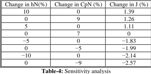
) = 9.32 + 0.72 and J = 784.32$.5. SENSITIVITY ANALYSIS
Here, a study has been made on the objective function due to the percentage change of holding cost and production cost. Table 3 gives the values of the objective function J for different values of hN and CPN, p = 1, 2. The percentage change
of these values is shown with respect to the values used in the previous example with h1, Cp1, h2,Cp2 and the minimum
objective value J = 776.79$. Table 4 shows that if hp and CpN are increased/decreased by +5%, +10%, −5% and −10%,
the values of the objective function change by 1.39% and 1.113%, 1.26% and 0%, −1.83% and −1.99% and −2.14% and −2.57% respectively.
The result shows that the production cost is more sensitive with respect to the holding cost.
Change in hN(%) Change in CpN (%) Change in J (%)
10 0 1.39
0 9 1.26
5 0 1.11
0 7 0
−5 0 −1.83
0 −5 −1.99
−10 0 −2.14
0 −9 −2.57
Table-4: Sensitivity analysis
6. CONCLUSIONS
For the given data, it is observed from Table 3 that the total cost is minimum for the model in cycle 5 and it is maximum for cycle 2.
Most of the optimal control production inventory problems are analyzed by considering the whole finite time horizon as a single cycle. But represent multi-cycles result indicates that the above consideration does not correspond to minimum cost. Here, the optimum minimum cost (776.79$) is due to four (4) cycles within the given time horizon and this cost is much lower than the cost (1449.02 $)with the whole time horizon as a single cycle.
REFERENCES
1. M.D.S. Aliyu, A.A Andhani, Multi-item-multi-plant inventory control of production systems with shortages/ backorders, International Journal of Systems Science 30 (1999) 533–539.
2. Z.T. Balkhi, On a finite horizon production lot size inventory model for deteriorating items and optimal solution, European Journal of Operational Research 132 (2001) 210–223.
3. Z.T. Balkhi, An optimal solution of a general lot inventory model with deteriorated and imperfect products, taking into account inflation and time value of money, International Journal of System Science 35 (2004) 87–96.
4. M. Bendaya, A. Rauof, On the constraint multi-item single period inventory problem, International Journal of Production Management 13 (1993) 104–112.
5. L. Benkherouf, A. Bomenir, L. Aggoun, A diffusion inventory model for deteriorating items, Applied Mathematics and Computation 138 (2003) 21–39.
6. S.E. El-gendi, Chebyshev solution of differential, integral and integro-differential equations, Computer Journal (1969) 282–287.
7. T.M. El-Gindy, H.M. El-Hawary, M.S. Salim, M. El-Kady, A Chebyshev approximation for solving optimal control problems, Computers & Mathematics with Applications 29 (1995) 35–45.
8. L. Fox, I.B. Parker, Chebyshev Polynomials in Numerical Analysis, University Press, Oxford, 1972.
9. S.K. Goyal, B.C. Giri, Recent trends modelling of deteriorating inventory, European Journal of Operational Research 134 (2001) 1–16.
10. M.A. Hariga, L. Benkherouf, Optimal and heuristic inventory replenishment models for deteriorating items with exponential time-varying demand, European Journal of Operational Research 79 (1994) 123–137.
11. F. Harris, Operations and Cost, in: Factory Management Series, A.W. Shaw co., Chicago, 1915.
12. L. Li, K.K. Lai, A fuzzy approach to the multi-objective transportation problem, Computers and Operations Research 27 (2000) 43–57.
13. K. Maity, M. Maiti, Production inventory system for deteriorating multi-item with inventory-dependent dynamic demands under inflation and discounting, Tamsui Oxford Journal of Management Sciences 21 (2005) 1–18.
15. K. Maity, M. Maiti, Inventory of deteriorating complementary and substitute items with stock dependent demand, American Journal of Mathematical and Management Science 25 (2005) 83–96.
16. Montevechi B. Arnaldo José, Pinho F. Alexandre, Salomon A. Valério, "Triangular Fuzzy Numbers Utilization in Flowshop Sequence Algorithm", Escola Federal de Engenharia de Itajubá , (1999) , Brazil . 17. E. Naddor, Inventory Systems, Wiley, New York, 1996.
18. G. Padmanabhan, P. Vrat, Analysis of multi-systems under resource constraint. A nonlinear Goal programming approach, Engineering Cost and Production Management 13 (1990) 104–112.
19. S. Sana, S.K. Goyal, K.S. Chaudhuri, A production-inventory model for a deteriorating item with trended demand and shortages, European Journal of Operational Research 157 (2004) 357–371.
20. B.M. Worell, M.A. Hall, The analysis of inventory control model using polynomial geometric programming, International Journal of Production Research 20 (1982) 657–667.
21. Y.Wu. Zhou, H.S. Lau, S.L. Yang, A new variable production scheduling strategy for deteriorating items with time-varying demand and partial lost sale, Computers and Operations research 30 (2003) 1753–1776.
Source of support: Nil, Conflict of interest: None Declared.