Comparative Analysis of LQG and LQGI Controllers for Twin Rotor MIMO System

1715

©IJRASET: All Rights are Reserved

Comparative Analysis of LQG and LQGI

Controllers for Twin Rotor MIMO System

Ch. S. Geetha Madhuri

1

_{, G. Raja Rao}

2

1_{M. Tech Student,} 2_{Professor and HOD, Department of Electrical and Electronics Engineering, ANITS}

Abstract: Twin Rotor MIMO system is an experimental model of Helicopter. It is a multi-input multi output system which is confined to two degree of freedom. It is utilized for the verification of controlling techniques and observers for helicopter manoeuvre. In this work Linear Quadratic Gaussian (LQG) controller and Linear Quadratic Gaussian controller with integral action (LQGI) are designed for the Twin Rotor MIMO system. Both control techniques are implemented for the control of Twin Rotor MIMO system, in MATLAB Simulink environment to check the endurance of each controller to meet the desired specifications.

Keywords: MIMO (Multiple Input Multiple Output) system, Manoeuvre, Linearization, Kalman Filter, LQG controller, LQGI controller.

I. INTRODUCTION

Twin rotor MIMO system is a boon to the Control Engineering Community who work on effectiveness of different control techniques for helicopter manoeuvre. It is cross coupled multiple input multiple output system. The aero dynamic model contains two rotors on each side of the horizontal beam. Both rotors are driven by individual DC motors. One rotor is known as main rotor and the other is tail rotor. The horizontal beam is counter balanced by pivoted beam. The horizontal beam can rotate in horizontal and vertical directions. Main rotor is responsible for up and down motion ,i.e it generates lifting force so that the horizontal beam is elevated about pitch axis. Tail rotor is responsible for the rotation of horizontal beam about yaw axis(vertical axis).

Various control approaches were implemented for the control of Twin Rotor Multiple Input Multiple Output system . In[2] PID control technique has been proposed for Twin Rotor System. In[3], authors defined the coupling effect and dynamic modelling of TRMS and cross coupled PID control was achieved using four PID controllers. In[4]Optimal control technique for TRMS was introduced and in[5] advanced adaptive control technique for twin rotor MIMO system was developed. In[6], the author compared the response of TRMS with PID and LQR controllers. In the present work, dynamic state space model of TRMS has been derived from differential equations. A Linear Quadratic Gaussian (LQG)controller and Linear Quadratic Gaussian controller with integral action(LQGI) have been designed separately. The response(steady state and transient) of the system is analysed for step input.

II. MATHEMATICAL MODELLING

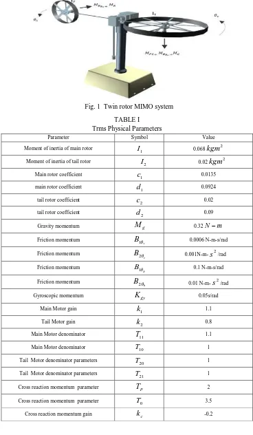
The mathematical model is derived from the model represented in Fig.1. The system can be represented by the set of differential equations. In vertical plane the differential equations can be given as,

G B FG v

M M M M dt d I

v 

 

 _



1 2 2 1

The characteristics of TRMS in vertical direction can be given by a second order equation which includes the torque induced ,

1 1 2 1 1

1 c d

M  

From the model shown in Fig.1, The gravitational momentum is induced due to rotation about vertical axis and it can be described by following equation,

v G

FG M

M  sin

The frictional torque is induced due to presence of frictional forces, so the estimation of frictional torque about the vertical axis can be explained by the differential equation followed,

             

dt d sign B dt d B

M v v

Bv v v

 

 

 1 2

Gyroscopic momentum is due to coriolis force in vertical direction can be given by the equation,

 

v h gy G

dt d M K

M 1  cos

1716

©IJRASET: All Rights are Reserved

[image:2.595.113.481.121.753.2]

Fig. 1 Twin rotor MIMO system

TABLE I Trms Physical Parameters

Parameter Symbol Value

Moment of inertia of main rotor

1

I

0.068

kgm

2

Moment of inertia of tail rotor

2

I

0.02

kgm

2

Main rotor coefficient

1

c

0.0135

main rotor coefficient

1

d

0.0924

tail rotor coefficient

2

c

0.02

tail rotor coefficient

2

d

0.09

Gravity momentum

M

_g 0.32Nm

Friction momentum

v

B

1_ 0.0006 N-m-s/rad

Friction momentum

v

B

2_

0.001N-m-2

s

/rad

Friction momentum

h

B

1 0.1 N-m-s/rad

Friction momentum

h

B

2_ 0.01 N-m-

s

2/rad

Gyroscopic momentum

K

_gy 0.05s/rad

Main Motor gain

k

₁ 1.1

Tail Motor gain

k

₂ 0.8

Main Motor denominator

T

₁₁ 1.1

Main Motor denominator

T

₁₀ 1

Tail Motor denominator parameters

T

₂₀ 1

Tail Motor denominator parameters

T

₂₁ 1

Cross reaction momentum parameter

T

_p 2

Cross reaction momentum parameter

T

₀ 3.5

1717

©IJRASET: All Rights are Reserved

The constants considered are TRMS parameters for the model considered are chosen experimentally .

The DC motor(main motor) and the electrical control circuit is approximated by the first order transfer function in Laplace domain given as, 1 10 11 1 1 u T s T k           

Similar equation is obtained in horizontal motion of the beam, so the balanced sum of moments in horizontal plane can be given as,

R B

h _{M M M}

dt d

I _  _h

       2 2 2 2

In horizontal plane the differential equations can be given as,

2 2 2 2 2

2 c d

M  

The frictional torque is induced due to presence of frictional forces, so the estimation of frictional torque about the horizontal axis can be explained by the differential equation followed

              dt d sign B dt d B

M v h

Bh h h

 

 

 1 2

The cross reaction momentum is approximated by the first order transfer function described by the equation below,









1

0 1 1       s s k M p c R

The DC motor(tail rotor) and the electrical control circuit is approximated by the first order transfer function in Laplace domain given as, 2 20 21 2 2 u T s T k         

From the above dynamic equations, the model can be represented by a set of differential equations from which state space model is obtained.

A. Jacobian Linearization

The mathematical model obtained in above section is non-linear and in order to design controller for system, the model should be linearized. The first step in linearization technique is to find equilibrium point.

Now Taylor series is applied to find equilibrium point. For this, make all differential equations equal to zero and find equilibrium

point. Take

u

₁=0 and

u

₂=0 and the equilibrium point is (0,0,0,0,0,0,0). Now, the variables x(t) and u(t) are related by the

differential equation x f(x(t),u(t))



.

Substituting in, using the constant and deviation variables, we get () ( (), ( ))

_ _ t u t x f

t x u

x  

   



By expanding , above equation can be written as _{() (}__,__{) () (t)}

u f t x f u x f

t _{x u}

x  

        

where _

            u u x x at x f

A , and _

     _{ }      u u x x at u f B ,

The non linear equations can be represented in state space form as shown below,

ẋ = AX+BU y = CX

Now let us consider output and state vector as,

T h v R h v dt d dt d M X _     

  , ,1,2,, ,  ,  and





T h v

1718

©IJRASET: All Rights are Reserved

                              0 5 50 5 . 4 0 0 0 0 08824 . 0 0 0 359 . 1 0 706 . 4 0 0 5 . 0 0 2182 . 0 0 0 0 0 0 1 0 0 0 0 0 0 0 9091 . 0 0 0 1 0 0 0 0 0 0 0 1 0 0 0 0 0 A                         0 0 0 0 0 35 . 0 8 . 0 0 0 1 0 0 0 0

B



_











0

0

0

0

0

1

0

0

0

0

0

0

0

1

C

By using A, B, C matrices TRMS system can be represented in state space form by using above state space equations. After representing the system in state space form, the next approach is to design the controller for the system to achieve desired output.

III.PROPOSED CONTROLLERS

A. Linear Quadratic Gaussian Controller

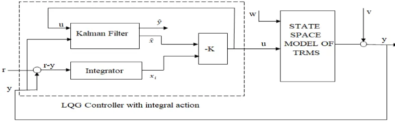
An LQG (Linear Quadratic Gaussian) Controller is an optimal controller which is a combined unit of Kalman Filter and Linear Quadratic Regulator. In this control technique Kalman filter is used to estimate all states of the system and Linear Quadratic Regulator controls the response of the system.

In[6], while designing LQR controller a full state feedback was assumed, which means all the states are available and can be measured directly, but in TRMS number of states are more than number of outputs. So all states present in the system can't be measured directly. Hence in this work, an observer is designed which estimates all states based on combination of input and output. The observer is Kalman Filter and it considers Process Noise and Measurement Noise and estimates the states. The LTI(linear time invariant) model of noisy plant can be represented as,

 

 

 

 

 

t Cx

 

t Du

 

t v

 

t y t w t F t Bu t Ax t x        ) (

Where

v

 

t

=Measuring Noise and

w

(

t

)

=Process Noise

The state-equation of Kalman Filter is given as, x0(t)A.x0(t)Bu(t)L(t)[y(t)Cx0(t)Du(t)]

[image:4.595.79.488.409.592.2]



Fig. 2 Block diagram of TRMS with LQG controller

So the overall noisy plant in state space model is given by following state and output equations,





(

)

(

)

)

(

0

0

t

A

BK

LC

LDK

x

t

Ly

t

x













)

(

)

(

t

Kx

₀

t

u





K is optimal regulator gain and the Kalman filter gain(L) can be given as , 0 1

R C V

L e T , The optimal regulator gain K which

minimizes the following quadratic cost function for continuous time,

 

_











0

.

dt

Ru

u

Qx

x

u

J

T T

1719

©IJRASET: All Rights are Reserved

Q and R matrices are estimated during the design process , The 'K' value is obtained by randomly varying diagonal elements of the Q and R matrices.

For the present work,



100

100

10

1

0

.

0001

10

^

4

100



diag

Q



and

_













1

0

0

100

R

The kalman gain is estimated by MATLAB command, [kest,L,P] = kalman (sys,w,v)

                            1234 . 9 4564 . 0 0459 . 0 0302 . 0 0459 . 0 0307 . 0 0535 . 0 0035 . 0 4896 . 0 1072 . 0 2707 . 4 0912 . 0 0912 . 0 2284 . 0 L

B. Linear Quadratic Gaussian Controller With Integral Action

A Linear Quadratic Gaussian Integral controller involves an addition of integral action to the LQG controlled TRMS. The system is subjected to disturbances w and v and is driven by control u. The integral LQG controller relies on noisy measurements y to generate the control signal u. The plant can be represented by state equations,

)

(

)

(

)

(

)

(

)

(

)

(

)

(

t

v

t

Du

t

Cx

y

t

w

t

F

t

Bu

t

Ax

x















[image:5.595.96.489.422.544.2]

Where

v

 

t

=Measuring Noise and

w

(

t

)

=Process Noise. Both v and w are called as White Noise.

Fig. 3 Block diagram of TRMS with LQGI controller

The LQG controller with integral action can be represented as,

                         0 0 i i x x i LDK BK LDK LC BK A x x



Kx Ki



u  

        i x x 

x

represents states estimated by Kalman Filter and

x

_i is Integrator output

To obtain optimal gain, following MATLAB command is used K= lqi(ss(A,B,C,D),Q,R)

1720

©IJRASET: All Rights are Reserved

 

_











0

.

dt

Ru

u

Qz

z

u

J

T T

For the present design, following Q and R matrices are considered below,

Qdiag



100 100 10 10 0.0001 10^4 10^4 10^6 10^6



and R=I. The Kalman gain is estimated by MATLAB command, [kest,L,P] = kalman (sys,w,v).

This command results the same vector of L which is obtained in LQG design as the Kalman filter estimates same states.

IV.SIMULATION RESULTS

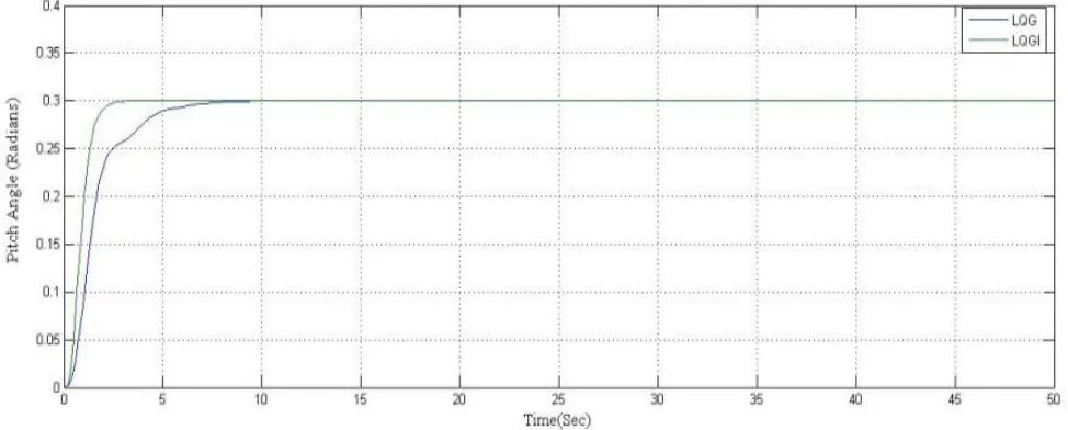
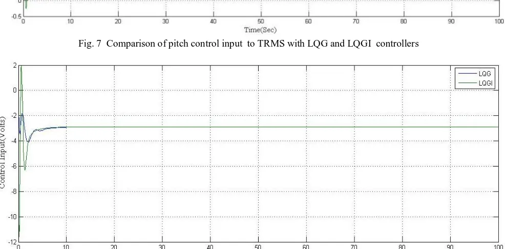
To implement the above control techniques mathematical model of TRMS is linearized and designed in Simulink. The controlled TRMS model is simulated. The response of the TRMS with the reference step input is observed. Transient response, steady state response are investigated through the parameters settling time, rise time, overshoot and steady state error. The reference signals are

and can be changed based on the requirement. Let =0.3 and = 0.5. So the reference step signals for pitch is 0.3 and for

[image:6.595.65.544.306.474.2]

yaw is 0.5 respectively.

Fig. FIG 4 Reference signals applied to TRMS U1=0.3 and U2=0.5

[image:6.595.57.544.513.709.2]

1721

[image:7.595.60.542.112.297.2]

©IJRASET: All Rights are Reserved

[image:7.595.56.549.330.504.2]

Fig. 6 Comparison of yaw response of TRMS with LQG and LQGI controller

Fig. 7 Comparison of pitch control input to TRMS with LQG and LQGI controllers

[image:7.595.55.548.472.715.2]

1722

©IJRASET: All Rights are Reserved

TABLE II Observations

Controller Parameter Rise time(

t

r) (Sec)

Settling Time(

t

_s)

(Sec)

%

M

_p % error

LQG Pitch 1.75 9 0 0

Yaw 1.0 6.5 0 0

LQGI Pitch 0.95 3.5 0 0

Yaw 0.9 3.5 0 0

V. CONCLUTION

In the present work an LQG controller and LQGI controllers were designed for TRMS model. This work involves the implementation and analysis of Linear Quadratic Gaussian controller and Linear Quadratic Gaussian controller with integral action for Twin Rotor MIMO system. It was already observed that Linear Quadratic Gaussian controller is giving the optimum response when compared to LQR controller. In the present work it was observed that the LQGI controller for TRMS results better response (in terms of time domain specifications)when compared to LQG controller for the same control energy.

REFERENCES

[1] TRMS 33-949S User Manual, Feedback instruments Ltd., East Sussex, U.K.(1998).

[2] Kannan PS, Ms Sheenu: PID Control of Twin Rotor MIMO System, In International Journal of Advanced Research in Basic Engineering Sciences and Technology(2017)

[3] A.P.S. Ramalakshmi, P.S. Manoharan, Non-linear Modeling and PID Control of Twin Rotor MIMO System, In proceedings of IEEE International conference on Advanced Communication Control and Computing Technologies (2012).

[4] Ahmad, S.M., Chipperfield, A.J., Tokhi, M.O.: Dynamic modelling and optimal control of a twin rotor MIMO system. In: Proceedings of IEEE national aerospace and electronics conference (NAECON’2000), pp. 391–398, Dayton, Ohio, USA (2000).

[5] Adaptive Control of Twin ROTOR MIMO System, Petr Chalupa, Jan Přikryl, Jakub Novák 2015 International Conference on Process Control (PC) June 9–12, Štrbské Pleso, Slovakia.(2015). (2002) The IEEE website. [Online]. Available: http://www.ieee.org/