Optimizing to Arbitrary NLP Metrics using Ensemble Selection

Optimizing to Arbitrary NLP Metrics using Ensemble Selection

Art Munson, Claire Cardie, Rich Caruana

Department of Computer Science Cornell University

Ithaca, NY 14850

{mmunson, cardie, caruana}@cs.cornell.edu

Abstract

While there have been many successful applica-tions of machine learning methods to tasks in NLP, learning algorithms are not typically designed to optimize NLP performance metrics. This paper evaluates an ensemble selection framework de-signed to optimize arbitrary metrics and automate the process of algorithm selection and parameter tuning. We report the results of experiments that in-stantiate the framework for three NLP tasks, using six learning algorithms, a wide variety of parame-terizations, and 15 performance metrics. Based on our results, we make recommendations for subse-quent machine-learning-based research for natural language learning.

1 Introduction

Among the most successful natural language learn-ing techniques for a wide variety of llearn-inguistic phe-nomena are supervised inductive learning algo-rithms for classification. Because of their capa-bilities for accurate, robust, and efficient linguistic knowledge acquisition, they have been employed in many natural language processing (NLP) tasks.

Unfortunately, supervised classification algo-rithms are typically designed to optimize accuracy (e.g. decision trees) or mean squared error (e.g. neu-ral networks). For many NLP tasks, however, these standard performance measures are inappropriate. For example, NLP data can be highly skewed in its distribution of positive and negative examples. In these situations, another metric (perhaps F-measure or a task-specific measure) that focuses on the per-formance of the minority cases is more appropriate. Indeed, as the NLP field matures more consideration will be given to evaluating the performance of NLP

components in context (e.g. Is the system easy to use by end users? Does the component respect user pref-erences? How well does the entire system solve the specific problem?), leading to new and complicated metrics. Optimizing machine learning algorithms to arbitrary performance metrics, however, is not easily done.

To exacerbate matters, the metric of interest might change depending on how the natural language learning (NLL) component is employed. Some ap-plications might need components with high re-call, for example; others, high precision or high F-measure or low root mean squared error. To obtain good results w.r.t. the new metric, however, a dif-ferent parameterization or difdif-ferent algorithm alto-gether might be called for, requiring re-training the classifier(s) from scratch.

Caruana et al. (2004) have recently proposed

semble selection as a technique for building an

en-semble of classifiers that is optimized to an arbitrary performance metric. The approach trains a large number of classifiers using multiple algorithms and parameter settings, with the idea that at least some of the classifiers will perform well on any given per-formance measure. The best set of classifiers, w.r.t. the target metric, is then greedily selected. (Select-ing a set of size 1 is equivalent to parameter and algorithm tuning.) Like other ensemble learning methods (e.g. bagging (Breiman, 1996) and boost-ing (Freund and Schapire, 1996)), ensemble selec-tion has been shown to exhibit reliably better perfor-mance than any of the contributing classifiers for a number of learning tasks.

In addition, ensemble selection provides an

lary benefit: no human expertise is required in se-lecting an appropriate machine learning algorithm or in choosing suitable parameter settings to get good performance. This is particularly attractive for the NLP community where researchers often rely on the same one or two algorithms and use default param-eter settings for simplicity. Ensemble selection is a tool usable by non-experts to find good classifiers optimized to task-specific metrics.

This paper evaluates the utility of the ensemble se-lection framework for NLL. We use three NLP tasks

for the empirical evaluation: noun phrase corefer-ence resolution and two problems from sentiment analysis — identifying private state frames and the hierarchy among them. The evaluation employs six learning algorithms, a wide selection of parameteri-zations, 8 standard metrics, and 7 task-specific met-rics. Because ensemble selection subsumes param-eter and algorithm selection, we also measure the impact of parameter and algorithm tuning.

Perhaps not surprisingly, we find first that no one algorithm or parameter configuration performs the best across all tasks or across all metrics. In ad-dition, an algorithm’s “tuned” performance (i.e. the performance after tuning parameter settings) almost universally matches or exceeds the algorithm’s de-fault performance (i.e. when using dede-fault parame-ter settings). Out of 154 total cases, the tuned clas-sifier outperforms the default clasclas-sifier 114 times, matches performance 28 times, and underperforms 12 times. Together, these results indicate the impor-tance of algorithm and parameter selection for com-parative empirical NLL studies. In particular, our results show the danger of relying on the same one or two algorithms for all tasks. These results cast doubt on conclusions regarding differences in algo-rithm performance for NLL experiments that give inadequate attention to parameter selection.

The results of our experiments that use ensem-ble selection to optimize the ensemensem-ble to arbitrary metrics are mixed. We see reliable improvements in performance across almost all of the metrics for only two of the three tasks; for the other data set, ensemble selection tends to hurt performance (al-though losses are very small). Perhaps more impor-tantly for our purposes, we find that ensemble se-lection provides small, but consistent gains in per-formance when considering only the more complex,

task-specific metrics — metrics that learning algo-rithms would find difficult to optimize.

The rest of the paper is organized as follows. Sec-tion 2 describes the general learning framework and provides an overview of ensemble selection. We present the particular instantiation of the framework employed in our experiments in Section 3. Section 4 describes the three NLP tasks. Experimental results are given in Section 5. Related work and conclu-sions follow (sections 6 and 7).

2 Ensemble Selection Framework

2.1 Terminology

We use the term model to refer to a classifier pro-duced by some learning algorithm using some par-ticular set of parameters. A model’s configuration is simply the algorithm and parameter settings used to create the classifier. A model family is the set of models made by varying the parameters for one ma-chine learning algorithm. Finally, a model library is a collection of models trained for a given task.

2.2 Framework

Abstractly, the framework is the following: 1. Select a variety of learning algorithms.

2. For each algorithm, choose a wide range of set-tings for the algorithm’s parameters.

3. Divide data into training, tuning, and test sets. 4. Build model library.

5. Select target metrics appropriate to problem. 6. Tune parameter settings and/or run ensemble

selection algorithm for target metrics.

Building the model library consists of (a) using the training data to train models for all the learning algorithms under all desired combinations of param-eter settings, and (b) applying each model to the tun-ing and test set instances and stortun-ing the predictions for use in step (6). Note that models are placed in the library regardless of performance, even though some models have very bad performance. Intuitively, this is because there is no way to know a priori which models will perform well on a given metric. Note that producing the base models is fully automatic and requires no expert tuning.

Parameter Tuning: The goal of parameter

the model from the model library with the highest performance on the tuning data and report its perfor-mance on the test data.

Ensemble Selection Algorithm: The ensemble

selection algorithm (Caruana et al., 2004) ignores model-specific details by only using the predictions

made by the models: the ensemble makes

predic-tions by averaging the predicpredic-tions of its constituents. Advantageously, this only requires that predictions made by different models fall in the same range, and that they can be averaged in a meaningful way. Oth-erwise, models can take any form, including other ensemble methods (e.g. bagging or boosting). Con-ceptually, ensemble selection builds on top of the models in the library and uses their performance as a starting point from which to improve.

The basic ensemble selection algorithm is: a. Start with an empty ensemble.

b. Add the model that results in the best perfor-mance for the current ensemble with respect to the tuning data and the target metric.

c. Repeat (b) for a large, fixed number of itera-tions.

d. The final ensemble is the ensemble from the best performing iteration on the tuning data for the target metric.

To prevent the algorithm from overfitting the tun-ing data we use two enhancements given by Caruana

et al. (2004). First, in step (b) the same model can be

selected multiple times (i.e. selection with replace-ment). Second, the ensemble is initialized with the topN models (again, with respect to the target met-ric on the tuning data). N is picked automatically such that removing or adding a model decreases per-formance on the tuning data.1

The main advantage to this framework is its reusability. After an instantiation of the framework exists, it is straightforward to apply it to multiple NLL tasks and to add additional metrics. Steps (1) and (2) only need to be done once, regardless of the number of tasks and metrics explored. Steps (3)-(5) need only be done once per NLL task. Importantly, the model library is created once for each task (i.e. each model configuration is only trained once) re-gardless of the number (or addition) of performance

1_{We also experimented with the bagging improvement}

de-scribed by Caruana et al. (2004). In our experiments using bag-ging hurt the performance of ensemble selection.

metrics. Finally, finding a classifier or ensemble op-timized to a new metric (step (6)) does not require re-building the model library and is very fast com-pared to training the classifiers—it only requires av-eraging the stored predictions. For example, training the model library for our smallest data set took mul-tiple days; ensemble selection built optimized en-sembles for each metric in a few minutes.

3 Framework Instantiation

In this section we describe our instantiation of the ensemble selection framework.

Algorithms: We use bagged decision trees (Breiman, 1996), boosted decision stumps (Fre-und and Schapire, 1996),k-nearest neighbor, a rule learner, and support vector machines (SVM’s). We use the following implementations of these algo-rithms, respectively: IND decision tree package (Buntine, 1993); WEKA toolkit (Witten and Frank, 2000); TiMBL (Daelemans et al., 2000); RIPPER (Cohen, 1995); andSVMlight(Joachims, 1999). Ad-ditionally, we use logistic regression (LR) for coref-erence resolution because an implementation using theMALLET(McCallum, 2002) toolkit was readily available for the task. The predictions from all algo-rithms are scaled to the range[0,1]with values close to 1 indicating positive predictions and values close to 0 indicating negative predictions.2

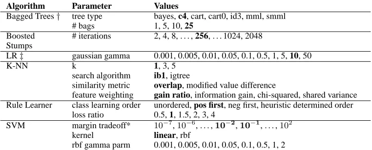
Parameter Settings: Table 1 lists the

parame-ter settings we vary for each algorithm. Additional domain-specific parameters are also varied for coref-erence resolution models (see Section 4.1). The model libraries contain models corresponding to the cross product of the various parameter settings for a given algorithm.

Standard Performance Metrics: We evaluate

the framework with 8 metrics: accuracy (ACC), average precision (APR), break even point (BEP), F-measure (F1), mean cross entropy (MXE), root mean squared error (RMS), area under the ROC curve (ROC), and SAR. Caruana et al. (2004) de-fine SAR asSAR= ACC+ROC+(1₃ −RM S). We also evaluate the effects of model selection with task-specific metrics. These are described in Section 4. Our F-measure places equal emphasis on precision

2_{We follow Caruana et al. (2004) in using Platt (2000)}

Algorithm Parameter Values

Bagged Trees† tree type bayes, c4, cart, cart0, id3, mml, smml

# bags 1, 5, 10, 25

Boosted Stumps

# iterations 2, 4, 8, . . . , 256, . . . 1024, 2048

LR‡ gaussian gamma 0.001, 0.005, 0.01, 0.05, 0.1, 0.5, 1, 5, 10, 50

K-NN k 1, 3, 5

search algorithm ib1, igtree

similarity metric overlap, modified value difference

feature weighting gain ratio, information gain, chi-squared, shared variance Rule Learner class learning order unordered, pos first, neg first, heuristic determined order

loss ratio 0.5, 1, 1.5, 2, 3, 4

SVM margin tradeoff* 10−7,10−6, . . . ,10−2,10−1, . . . ,102

kernel linear, rbf

rbf gamma parm 0.001, 0.005, 0.01, 0.05, 0.1, 0.5, 1, 2

Table 1: Summary of model configurations used in experiments. The default settings for each algorithm are in bold. †Bagged trees are not used for identifying PSF’s since the IND package does not support features with more than 255 values. Also, for coreference resolution the number of bags is not varied and is always 25. ‡LR is only used for coreference resolution. *SVMlightdetermines the default margin tradeoff based on data properties. We calculate this value for each data set and use the closest setting among our configurations.

and recall (i.e.β = 1). Note that precision and re-call are calculated with respect to the positive class.

Ensemble Selection: For the sentiment analysis

tasks, ensemble selection iterates 150 times; for the coreference task, the algorithm iterates 200 times. This should be enough iterations, given that the model libraries contain 202, 173, and 338 mod-els. Because computing the MUC-F1 and BCUBED metrics (see Section 4.1) is expensive, ensemble se-lection only iterates 50 times for these metrics.

4 Tasks

Because of space issues, we necessarily provide only brief descriptions of each NLL task. Readers are referred to the cited papers to obtain detailed de-scriptions.

4.1 Noun Phrase Coreference Resolution

The goal for a standard noun phrase coreference res-olution system is to identify the noun phrases in a document and determine which of them refer to the same entity. Entities can be people, places, things,

etc. The resulting partitioning of noun phrases

cre-ates reference chains with one chain per entity. We use the same problem formulation as Soon et

al. (2001) and Ng and Cardie (2002) — a

combi-nation of classification and clustering. Briefly, ev-ery noun phrase is paired with all preceding noun phrases, creating multiple pairs. For the training data, the pairs are labeled as coreferent or not. A binary classifier is trained to predict the pair labels. During classification, the predicted labels are used

to form clusters. Two noun phrasesA andB share a cluster if they are either predicted as coreferent by the classifier or if they are transitively predicted as coreferent through one or more other noun phrases. Instance selection (Soon et al., 2001; Ng, 2004) is used to increase the percentage of positive instances in the training set.3

We use the learning features described by Ng and Cardie (2002). All learning algorithms are trained with the full set of features. Additionally, the rule learner, SVM, and LR are also trained with a hand-selected subset of the features that Ng and Cardie (2002) find to outperform the full feature set. Essentially this is an additional parameter to set for the learning task.

Special Metrics: Rather than focusing on

per-formance at the pairwise coreference classification level, performance for this task is typically reported using either the MUC metric (Vilain et al., 1995) or the BCUBED metric (Bagga and Baldwin, 1998). Both of these metrics measure the degree that pre-dicted coreference chains agree with an answer key. In particular they measure the chain-level precision and recall (and the corresponding F-measure). We abbreviate these metrics MUC-F1, and B3F1.

Data Set: For our experiments we use the

MUC-6 corpus, which contains MUC-60 documents annotated with coreference information. The training, tuning, and test sets consist of documents 1-20, 21-30, and

3_{Soon-1instance selection is used for all algorithms; we}

31-60, respectively.

4.2 Identifying Private State Frames

NLP research has recently started looking at how to detect and understand subjectivity in discourse. A key step in this direction is automatically identi-fying phrases that express subjectivity. In this set-ting, subjectivity is defined to include implicit and explicit opinions, internal thoughts and emotions, and bias introduced through second-hand reporting. Phrases expressing any of these are called private

state frames, which we will abbreviate as PSF.

We build directly on experiments done by Wiebe

et al. (2003). The task is to learn to identify explicit

single-word PSF’s in context. One learning instance is created for every word in the corpus. Classifica-tion labels each instance as a PSF or not. We use the same features as Wiebe et al.

Special Metrics: Because the data is highly skewed (2% positive instances), performance mea-sures that focus on how well the minority class is learned are of primary interest. The F-measure de-fined in Section 3 is a natural choice. We also eval-uate performance using geometric accuracy, defined asGACC =√posacc×negaccwhereposaccand

negaccare the accuracy with respect to the positive and negative instances (Kubat and Matwin, 1997).

Conceivably, an automatic PSF extractor with high precision and mediocre recall could be used to automate the annotation process. For this reason we measure the performance with an unbalanced F-measure that emphasizes precision. Specifically, we tryβ = 0.5(F0.5) andβ = 0.2(F0.2).

Data Set: We use 400 documents from the MPQA corpus (2002), a collection of news stories manually annotated with PSF information. The 400 documents are randomly split to get 320 training, 40 tuning, and 40 testing documents.

4.3 Determining PSF Hierarchy

The third task is taken from Breck and Cardie (2004). Explicit PSF’s each have a source that cor-responds to the person or entity expressing the sub-jectivity. In the presence of second-hand reporting, sources are often nested. This has the effect of filter-ing subjectivity through a chain of sources.

Given sentences annotated with PSF information (i.e. which spans are PSF’s), the task is to discover

the hierarchy among the PSF’s that corresponds to the nesting of their respective sources. From each sentence, multiple instances are created by pair-ing every PSF with every other PSF in the sen-tence.4 Let(P SFparent, P SFtarget)denote one of

these instances. The classification task is to decide if P SFparent is the parent ofP SFtarget in the

hi-erarchy and to associate a confidence with that pre-diction. The complete hierarchy can easily be con-structed from the predictions by choosing for each PSF its most confidently predicted parent.

Special Metrics: Breck and Cardie (2004)

mea-sure task performance with three metrics. The first is the accuracy of the predictions over the instances. The second is a derivative of a measure used to score dependency parses. Essentially, a sentence’s score is the fraction of parent links correctly identified. The score for a set of sentences is the average of the indi-vidual sentence scores. We refer to this measure as average sentence accuracy (SENTACC). The third measure is the percentage of sentences whose hier-archical structures are perfectly determined (PERF-SENT).

Data Set: We use the same data set and

fea-tures as Breck and Cardie (2004). The annotated sentences from 469 documents in the MPQA Cor-pus (MPQA CorCor-pus, 2002) are randomly split into training (80%), tuning (10%), and test (10%) sets.

5 Experiments and Results

We evaluate the potential benefits of the ensemble selection framework with two experiments. The first experiment measures the performance improvement yielded by parameter tuning and finds the best per-forming algorithm. The second experiment mea-sures the performance improvement from ensemble selection.

Performance improvements are measured in terms of performance gain. Letaandbbe the mea-sured performances for two models A and B on some metric. A’s gain overB is simply a−b. A

performed worse thanB if the gain is negative.5

4_{Sentences containing fewer than two PSF’s are discarded}

and not used.

5_{MXE and RMS have inverted scales where the best}

Metric BAG Parm∆ BST Parm∆ LR Parm∆ KNN Parm∆ RULE Parm∆ SVM Parm∆ Avg∆

ACC 0.9861 -0.0000 0.9861 -0.0001 0.9849 0.0006 0.9724 0.0131 0.9840 0.0023 0.9859 -0.0001 0.0026 APR 0.5373 0.0000 0.5475 0.0000 0.3195 -0.0004 0.1917 0.2843 0.2491 0.1127 0.5046 0.0323 0.0715 BEP 0.6010 0.0000 0.5577 0.0193 0.3747 -0.0022 0.3243 0.2057 0.3771 0.1862 0.5965 0.0045 0.0689 F1 0.5231 0.0664 0.3881 0.0000 0.4600 0.0087 0.4105 0.1383 0.4453 0.1407 0.3527 0.0571 0.0685 MXE 0.9433 0.0082 0.9373 0.0000 0.5400 0.1828 0.4953 0.3734 0.9128 0.0222 0.9366 0.0077 0.0990 RMS 0.8925 0.0041 0.8882 0.0000 0.6288 0.1278 0.8334 0.0559 0.8756 0.0097 0.8859 0.0047 0.0337 ROC 0.9258 0.0158 0.9466 0.0000 0.4275 0.0022 0.7746 0.0954 0.6845 0.1990 0.8418 0.0551 0.0612 coreference SAR 0.9255 0.0069 0.9309 0.0000 0.6736 -0.0037 0.8515 0.0538 0.8396 0.0695 0.8955 0.0165 0.0238 MUC-F1 0.6691 0.0000 0.6242 0.0046 0.6405 0.0344 0.5340 0.1185 0.6500 0.0291 0.5181 0.1216 0.0514 B3F1 0.4625 0.0000 0.4512 0.0000 0.4423 0.0425 0.0965 0.3357 0.4249 0.0675 0.3323 0.1430 0.0981 ACC — — 0.9854 0.0007 — — 0.9873 0.0011 0.9862 0.0003 0.9886 0.0000 0.0005 APR — — 0.6430 0.0316 — — 0.5588 0.1948 0.4335 0.0381 0.7697 0.0372 0.0754 BEP — — 0.5954 0.0165 — — 0.6727 0.0302 0.4436 0.0718 0.6961 0.0385 0.0393 F1 — — 0.5643 0.0276 — — 0.6837 0.0019 0.5770 0.0367 0.6741 0.0062 0.0181 MXE — — 0.9342 0.0029 — — 0.8089 0.1425 0.9265 0.0062 0.9572 0.0093 0.0402 RMS — — 0.8838 0.0028 — — 0.8896 0.0118 0.8839 0.0020 0.9000 0.0068 0.0058 ROC — — 0.9576 0.0121 — — 0.8566 0.1149 0.7181 0.1593 0.9659 0.0188 0.0763

PSF

identification

SAR — — 0.9329 0.0052 — — 0.9021 0.0407 0.8541 0.0532 0.9420 0.0085 0.0269 GACC — — 0.6607 -0.0004 — — 0.7962 0.0223 0.6610 0.0506 0.7401 0.0209 0.0233 F0.5 — — 0.6829 0.0221 — — 0.7150 0.0503 0.7132 0.0000 0.7811 -0.0054 0.0167 F0.2 — — 0.7701 0.0157 — — 0.7331 0.0875 0.8171 0.0110 0.8542 0.0045 0.0297 ACC 0.8133 0.0000 0.7554 0.0009 — — 0.7940 0.0000 0.7446 0.0428 0.7761 0.0381 0.0164 APR 0.8166 0.0296 0.7455 0.0013 — — 0.8035 0.0000 0.5957 0.1996 0.6363 0.1520 0.0765 BEP 0.7385 -0.0066 0.6597 -0.0030 — — 0.7096 0.0000 0.6317 0.0567 0.6940 0.0432 0.0181 F1 0.7286 0.0033 0.6810 0.0226 — — 0.7000 0.0000 0.6774 0.0525 0.6933 0.0400 0.0237 MXE 0.6091 0.0166 0.4940 0.0076 — — 0.0379 0.4715 0.4022 0.1197 0.4681 0.1012 0.1433 RMS 0.6475 0.0054 0.5910 0.0033 — — 0.6057 0.0000 0.5556 0.0514 0.5836 0.0423 0.0205 ROC 0.8923 0.0096 0.8510 0.0000 — — 0.8519 0.0364 0.7514 0.1094 0.7968 0.0757 0.0462

PSF

hierarch

y

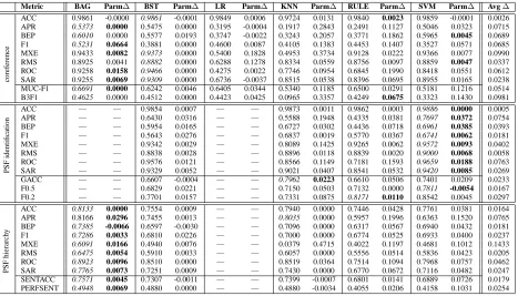
SAR 0.7765 0.0073 0.7251 0.0009 — — 0.7430 0.0000 0.6770 0.0672 0.7116 0.0482 0.0247 SENTACC 0.7571 0.0045 0.7307 -0.0011 — — 0.7399 -0.0007 0.6801 0.0141 0.6889 0.0726 0.0179 PERFSENT 0.4948 0.0069 0.4880 0.0000 — — 0.4880 -0.0034 0.4055 0.0206 0.4158 0.1031 0.0254 Table 2: Performance gains from parameter tuning. The left column for each algorithm family is the algorithm’s performance with default parameter settings. The adjacent ‘Parm∆’ column gives the performance gain from tuning parameters. For each metric, the best default and tuned performance across all algorithms are italicized and bold-faced, respectively.

5.1 Experiment 1: Parameter Tuning

Experiment 1 measures, for each of the 3 tasks, the performance of every model on both the tuning and test data for every metric of interest. Based on

tun-ing set performance, the best default model, the best

model overall, and the best model within each fam-ily are selected. The best default model is the highest-scoring model that emerges after comparing algorithms without doing any parameter tuning. The

best overall model corresponds to “tuning” both the

algorithm and parameters. The best model in each

family corresponds to “tuning” the parameters for

that algorithm. Using the test set performances, the best family models are compared to the correspond-ing default models to find the gains from parameter tuning.

Table 2 lists the gains achieved by parameter tun-ing. Each algorithm column compares the algo-rithm’s best model to its default model. On the coreference task, for example, the best KNN model with respect to BEP shows a 20% improvement (or gain) over the default KNN model (for a final BEP score of .5300). The “Avg∆” column shows the av-erage gain from parameter tuning for each metric.

For each metric, the best default model is

itali-cized while the best overall model is bold-faced. Re-ferring again to the coreference BEP row, the best overall model is a SVM while the best default model is a bagged decision tree. Recall that these distinc-tions are based on absolute performance and not gain. Thus, the best tuned SVM outperforms all other models on this task and metric.6

Three conclusions can be drawn from Table 2.

First, no algorithm performs the best on all tasks or on all metrics. For coreference, the best

over-all model is either a bagged tree, a rule learner, or a SVM, depending on the target metric. Similarly, for PSF identification the best model depends on the metric, ranging from a KNN to a SVM. Interest-ingly, bagged decision trees on the PSF hierarchy data outperform the other algorithms on all metrics and seem especially well-suited to the task.

Second, an algorithm’s best-tuned model reliably yields non-trivial gains over the corresponding de-fault model. This trend appears to hold regardless of

algorithm, metric, and data set. In 114 of the 154

6

cases parameter tuning improves an algorithm’s per-formance by more than 0.001 (0.1%). In the remain-ing 40 cases, parameter tunremain-ing only hurts 12 times, and never by more than 0.01.

Third, the best default algorithm is not necessar-ily the best algorithm after tuning parameters. The

coreference task, in particular, illustrates the poten-tial problem with using default parameter settings when judging which algorithm is most suited for a problem: 7 out of 10 times the best algorithm changes after parameter tuning.

These results corroborate those found else-where (Daelemans and Hoste, 2002; Hoste et al., 2002; Hoste, 2005)—parameter settings greatly in-fluence performance. Further, algorithmic perfor-mance differences can change when parameters are changed. Going beyond previous work, our results also underline the need to consider multiple algo-rithms for NLL. Ultimately, it is important for re-searchers to thoroughly explore options for both al-gorithm and parameter tuning and to report these in their results.

5.2 Experiment 2: Ensemble Selection

In experiment 2 an ensemble is built to optimize each target metric. The ensemble’s performance is compared to that of the best overall model for the metric. Both the ensemble and the best model are selected according to tuning set performance.

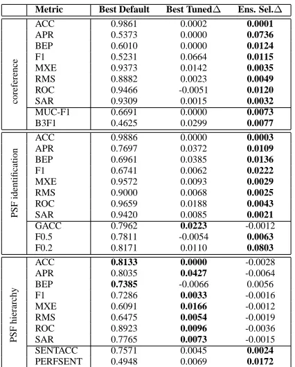
Table 3 lists the gains from ensemble selection over the best parameter tuned model. For compar-ison, the best default and overall performances from Table 2 are reprinted. For example, the ensemble op-timized for F1 on the coreference data outperforms the best bagged tree model by about 1% (and the best default model by almost 8%).

Disappointingly, ensemble selection does not consistently improve performance. Indeed, for the PSF hierarchy task ensemble selection reliably hurts performance a small amount. For the other two tasks ensemble selection reliably improves all metrics ex-cept GACC (a small loss). In other experiments, however, we optimized F-measure withβ = 1.5for the PSF identification task. Ensemble selection hurt F1.5 by almost 2%, leading us to question the tech-nique’s reliability for our second data set. Interest-ingly, the aggregate metrics—metrics that measure performance by combining multiple predictions—

Metric Best Default Best Tuned∆ Ens. Sel.∆

ACC 0.9861 0.0002 0.0001

APR 0.5373 0.0000 0.0736

BEP 0.6010 0.0000 0.0124

F1 0.5231 0.0664 0.0115

MXE 0.9373 0.0142 0.0035

RMS 0.8882 0.0023 0.0049

ROC 0.9466 -0.0051 0.0120

coreference SAR 0.9309 0.0015 0.0032

MUC-F1 0.6691 0.0000 0.0073

B3F1 0.4625 0.0299 0.0077

ACC 0.9886 0.0000 0.0003

APR 0.7697 0.0372 0.0109

BEP 0.6961 0.0385 0.0136

F1 0.6741 0.0062 0.0222

MXE 0.9572 0.0093 0.0029

RMS 0.9000 0.0068 0.0025

ROC 0.9659 0.0188 0.0043

PSF

identification

SAR 0.9420 0.0085 0.0021

GACC 0.7962 0.0223 -0.0012

F0.5 0.7811 -0.0054 0.0063

F0.2 0.8171 0.0110 0.0803

ACC 0.8133 0.0000 -0.0028

APR 0.8035 0.0427 -0.0064

BEP 0.7385 -0.0066 0.0056

F1 0.7286 0.0033 -0.0016

MXE 0.6091 0.0166 -0.0012

RMS 0.6475 0.0054 -0.0019

ROC 0.8923 0.0096 -0.0036

PSF

hierarch

y

SAR 0.7765 0.0073 -0.0015

SENTACC 0.7571 0.0045 0.0024 PERFSENT 0.4948 0.0069 0.0172

Table 3: Impact from tuning and ensemble selection.

Best default shows the performance of the best classifier with

no parameter tuning (i.e. algorithm tuning only). Best tuned∆ gives the performance gain from parameter and algorithm tun-ing. Ens. Sel.∆is the performance gain from ensemble selec-tion over the best tuned model. The best performance for each metric is marked in bold.

all benefit from ensemble selection, even for the hi-erarchy task, albeit for small amounts. For our tasks these comprise a subset of the task-specific perfor-mance measures: B3F1, MUC-F1, SENTACC, and PERFSENT.

While we are not surprised that the positive gains are small,7 we are surprised at how often ensemble selection hurts performance. As a result, we investi-gated some of the metrics where ensemble selection hurts performance and found that ensemble selec-tion overfits the tuning data. At this time we are not sure why this overfitting happens for these tasks and not for the ones used by Caruana et al. Preliminary investigations suggest that having a smaller model library is a contributing factor (Caruana et al. use libraries containing ∼ 2000 models). This is con-sistent with the fact that the task with the largest model library, coreference, benefits the most from ensemble selection. Perhaps the reason that ensem-ble selection consistently improves performance for

7_{Caruana et al. (2004) find the benefit from ensemble}

the aggregate metrics is that these metrics are harder to overfit.

Based on our results, ensemble selection seems too unreliable for general use in NLL—at least un-til the model library requirements are better under-stood. However, ensemble selection is perhaps trust-worthy enough to optimize metrics that are difficult to overfit and could not be easily optimized other-wise — in our case, the task-specific aggregate per-formance measures.

6 Related Work

Hoste et al. (2002) and Hoste (2005) study the im-pact of tuning parameters for k-NN and a rule-learning algorithm on word sense disambiguation and coreference resolution, respectively, and find that parameter settings greatly change results. Simi-lar work by Daelemans and Hoste (2002) shows the fallacy of comparing algorithm performance without first tuning parameters. They find that the best algo-rithm for a task frequently changes after optimizing parameters. In contrast to our work, these earlier experiments investigate at most two algorithms and only measure performance with one metric per task.

7 Conclusion

We evaluate an ensemble selection framework that enables optimizing classifier performance to arbi-trary performance metrics without re-training. An important side benefit of the framework is the fully automatic production of base-level models, remov-ing the need for human expertise in choosremov-ing algo-rithms and parameter settings.

Our experiments show that ensemble selection, compared to simple algorithm and parameter tuning, reliably improves performance for six of the seven task-specific metrics and all four “aggregate” met-rics, but only benefits all of the metrics for one of our three data sets. We also find that exploring mul-tiple algorithms with a variety of settings is impor-tant for getting the best performance. Tuning pa-rameter settings results in 0.05% to 14% average improvements, with most improvements falling be-tween 2% and 10%. To this end, the ensemble selec-tion framework can be used as an environment for automatically choosing the best algorithm and pa-rameter settings for a given NLP classification task.

More work is needed to understand when ensemble selection can be safely used for NLL.

Acknowledgements We thank Alex Niculescu-Mizil for answering questions about ensemble selection and Eric Breck for sharing his expertise with both PSF data sets. We also thank

the anonymous reviewers and the Cornell NLP group for help-ful suggestions on paper drafts. This work was supported by the Advanced Research and Development Activity (ARDA), by NSF Grant IIS-0208028, and by NSF Grant IIS-0412930.

References

Amit Bagga and Breck Baldwin. 1998. Algorithms for scoring coreference chains. In Linguistic Coreference Workshop at LREC 1998, pages 563–566, May.

Eric Breck and Claire Cardie. 2004. Playing the telephone game: Determining the hierarchical structure of perspective and speech expressions. In COLING

2004, pages 120–126.

Leo Breiman. 1996. Bagging predictors. Machine Learning, 24(2):123–140. Wray Buntine. 1993. Learning classification trees. In D. J. Hand, editor, Artificial

Intelligence Frontiers in Statistics, pages 182–201. Chapman & Hall, London.

Rich Caruana, Alexandru Niculescu-Mizil, Geoff Crew, and Alex Ksikes. 2004. Ensemble selection from libraries of models. In ICML.

William W. Cohen. 1995. Fast effective rule induction. In Armand Prieditis and Stuart Russell, editors, ICML, pages 115–123, Tahoe City, CA, July 9–12. Morgan Kaufmann.

Walter Daelemans and V´eronique Hoste. 2002. Evaluation of machine learning methods for natural language processing tasks. In LREC 2002, pages 755– 760.

Walter Daelemans, Jakub Zavrel, Ko van der Sloot, and Antal van den Bosch. 2000. TiMBL: Tilburg memory based learner, version 3.0, reference guide. ILK Technical Report 00-01, Tilburg University. Available from

http://ilk.kub.nl/˜ilk/papers/ ilk0001.ps.gz. Yoav Freund and Robert E. Schapire. 1996. Experiments with a new boosting

algorithm. In ICML, pages 148–156.

V´eronique Hoste, Iris Hendrickx, Walter Daelemans, and Antal van den Bosch. 2002. Parameter optimization for machine learning of word sense disam-biguation. Natural Language Engineering, 8(4):311–325.

V´eronique Hoste. 2005. Optimization Issues in Machine Learning of Coreference

Resolution. Ph.D. thesis, University of Antwerp.

Thorsten Joachims. 1999. Making large-scale SVM learning practical. In Bern-hard Sch¨olkopf, Christopher J. C. Burges, and Alexander J. Smola, editors,

Advances in Kernel Methods - Support Vector Learning. MIT Press,

Cam-bridge, USA.

Miroslav Kubat and Stan Matwin. 1997. Addressing the curse of imbalanced training sets: One-sided selection. In ICML, pages 179–186, San Francisco, CA. Morgan Kaufmann.

Andrew Kachites McCallum. 2002. MALLET: A machine learning for language toolkit.http://mallet.cs.umass.edu.

MPQA Corpus. 2002. NRRC MPQA corpus. Available fromhttp://nrrc. mitre.org/NRRC/Docs Data/MPQA 04/approval time.htm. Vincent Ng and Claire Cardie. 2002. Improving machine learning approaches to

coreference resolution. In ACL, pages 104–111.

Vincent Ng. 2004. Improving Machine Learning Approaches to Noun Phrase

Coreference Resolution. Ph.D. thesis, Cornell University.

John C. Platt. 2000. Probabilistic outputs for support vector machines and com-parison to regularized likelihood methods. In Alexander J. Smola, Peter J. Bartlett, Bernhard Schoelk¨opf, and Dale Schuurmans, editors, Advances in

Large-Margin Classifiers, pages 61–74. MIT Press.

Wee Meng Soon, Hwee Tou Ng, and Chung Yong Lim. 2001. A machine learning approach to coreference resolution of noun phrases. Computational

Linguis-tics, 27(4):521–544.

Marc Vilain, John Burger, John Aberdeen, Dennis Connolly, and Lynette Hirschman. 1995. A model-theoretic coreference scoring scheme. In Proc.

of the 6th Message Understanding Conference, pages 45–52. Morgan

Kauf-mann.

Janyce Wiebe, Eric Breck, Chris Buckley, Claire Cardie, Paul Davis, Bruce Fraser, Diane Litman, David Pierce, Ellen Riloff, Theresa Wilson, David Day, and Mark Maybury. 2003. Recognizing and organizing opinions expressed in the world press. In Papers from the AAAI Spring Symposium on New Directions

in Question Answering (AAAI tech report SS-03-07). March 24-26, 2003.

Stanford University, Palo Alto, California.

Ian H. Witten and Eibe Frank. 2000. Data Mining: Practical Machine Learning