Cluster-based collection selection
in uncooperative distributed
information retrieval
Bertold van Voorst MSc. Thesis July 7, 2010
University of Twente Department of Computer Science
Abstract
Background The focus of this research is collection selection for
dis-tributed information retrieval. The collection descriptions that are necessary for selecting the most relevant collections are often created from information gathered by random sampling. Collection selection based on an incomplete index constructed by using random sampling instead of a full index leads to inferior results.
Contributions In this research we propose to use collection clustering to compensate for the incompleteness of the indexes. When collection clustering is used we do not only select the collections that are considered relevant based on their collection descriptions, but also collections that have similar content in their indexes. Most existing cluster algorithms require the specication of the number of clusters prior to execution. We describe a new clustering algorithm that allows us to specify the sizes of the produced clusters instead of the number of clusters.
Conclusions Our experiments show that that collection clustering can
Acknowledgments
Contents
Abstract i
Acknowledgments iii
1 Introduction 1
1.1 Information retrieval . . . 1
1.2 Centralized search . . . 2
1.3 Distributed information retrieval . . . 2
1.4 Collection selection based on content similarity . . . 3
1.5 Research questions . . . 5
1.6 Thesis outline . . . 7
2 Literature 9 2.1 Zipf's law . . . 9
2.2 Query-based sampling . . . 10
2.3 Cluster hypothesis . . . 11
2.4 Collection selection algorithms . . . 12
2.4.1 GlOSS . . . 12
2.4.2 Cue Validity Variance . . . 13
2.4.3 CORI . . . 14
2.4.4 Indri . . . 15
2.4.5 Discussion . . . 16
2.5 Clustering . . . 16
2.5.1 Clustering types . . . 17
2.5.2 K-means algorithm . . . 17
2.5.3 Bisecting k-means algorithm . . . 19
2.6 Cluster-based retrieval . . . 20
2.7 Summary . . . 21
3 Research 23 3.1 The WT10g corpus . . . 23
3.2 Random sampling . . . 25
3.3 Clustering . . . 26
3.3.2 K-means . . . 26
3.3.3 Bisecting k-means . . . 27
3.3.4 Indexing clusters . . . 28
3.4 Ranking collections . . . 28
3.5 Evaluation . . . 29
3.6 Summary . . . 31
4 Results 33 4.1 Query-based sampling . . . 33
4.2 Cluster sizes and the number of clusters . . . 34
4.3 Cluster quality . . . 39
4.4 Comparing cluster algorithms . . . 40
4.5 Query sets . . . 42
4.6 Summary . . . 43
5 Conclusion 45 5.1 Collection selection algorithms . . . 45
5.2 Incomplete resource descriptions . . . 46
5.3 Measuring collection selection performance . . . 46
5.4 Cluster methods . . . 47
5.5 Using clustering to improve collection selection . . . 47
5.6 Summary . . . 48
6 Future work 49 6.1 Replacing CORI . . . 49
6.2 Conducting experiments using dierent corpora . . . 49
6.3 Improving performance . . . 50
Bibliography 51
A Bisecting k-means recall and precision 57
B K-means recall and precision 65
C K-means and bisecting k-means 67
Chapter 1
Introduction
Distributed information retrieval is a promising technique to improve the quality and scalability of web search. A major part of distributed information retrieval is collection selection. We propose to use collection clustering to improve the performance of existing collection selection algorithms.
1.1 Information retrieval
One of the web's most important applications is search. People who use web search engines have an information need, that is expressed by a query. The query is a short description of the information need, usually consisting of a single or a few words. The goal of the search engine is to return a list of web pages that best match the information need as described by the user's query, ranked by estimated relevance.
In order to do this, a search engine needs information about the doc-uments that are available on the web. This information is gathered by a process called crawling, in which web pages are retrieved and stored. The most common way to make all the retrieved information easily searchable, is by creating an index which keeps track of the words that each document contains.
The matching of a user query against the documents that are present in an index, is much like looking up a word in the index in the back of a book. Retrieval methods have been developed that not only select the documents that contain the query words but also rank them by relevance. A very
popular method is tf ·idf which uses the number of occurrences of a word
1.2 Centralized search
Web search is currently dominated by centralized search engines. These search engines use a single large index for searching purposes. Even though the services may run on a large distributed cluster the control over the data is still centralized. Centralized control can be an advantage for large companies like Google or Yahoo, but it also has a number of disadvantages.
Crawling, indexing and searching a considerable part of the web requires a huge amount of resources. Even the biggest search engines index only a small part of the web. In 2005, the four biggest search engines together had indexed no more than 30% of the total visible web pages [16]. These numbers are only about the surface web. The deep or invisible web consists of pages that are hidden behind the query forms of searchable databases.
For example: web pages that use AJAX1 for displaying dynamic content to
the user. Automatic web crawlers often can not access this data since they are not able to ll in and submit web forms. The deep web is estimated to be 500 times larger than the surface web [17].
Due to the size and dynamic nature of the web it is very hard, if not impossible, to keep a large index fresh. Changes in web pages are not noticed until the page is crawled again.
A non-technical issue is the monopoly of large search engines. A few companies control the way we can search information on the web and, as a result, can control which information becomes publicly available [22].
1.3 Distributed information retrieval
In distributed information retrieval -also called federated search or metasearch-a broker sends metasearch-a query to multiple semetasearch-arch engines metasearch-at the smetasearch-ame time. These search engines may use classic search indexes that contain the web pages, but may also have direct access to the data that is hidden behind web forms. When web pages are dynamically generated from data in a database, a search engine can search in this database instead of searching in an index based on previously generated web pages. Each collection evaluates the query and returns the results to the broker. The broker then merges the results and presents them to the user as a single result list. Distributed search consists of three steps: collection description, collection selection and results merging. An overview of this process is show in Figure 1.1.
Collection description Collection description is the task where the bro-ker learns which collection are available and what information is contained by each collection. Collection descriptions are mostly built on statistics
Client
Broker
Collection 1 Collection 2 Collection i Collection n-1 Collection n 1. Query
2. Query 2. Query
3. Results 3. Results
[image:11.595.153.392.123.299.2]4. Merged results
Figure 1.1: The broker forwards a query to a number of collections and returns the merged result list. Image taken from [6].
about word distributions in the collection, but can also contain information obtained from the search engine's interface or manually added metadata.
Collection selection A distributed search engine may be able to direct queries to thousands of search engines. Sending a user query to all of them will generate too much overhead. Therefore the broker must select a limited number of search engines to use. This task is called collection selection. The main goal is to select only those collections that will return the most relevant results in response to the user's query.
Results merging When the results from the search engines are returned to the broker the results must be merged. Duplicate results are removed and a single result list is generated, typically ordered by relevance. Merging algorithms can use a wide range of available information about the retrieved results, from their local ranks, their titles and snippets, to the full documents of these results [25].
1.4 Collection selection based on content similarity
Collection selection algorithms mostly depend on content summaries derived from the search engines they address. These content summaries can be retrieved in two possible ways.
trust the search engines, because they might intentionally or unintentionally provide incorrect descriptions.
Second, resource descriptions can be obtained by random sampling tech-niques such as query-based sampling [8]. Queries are sent to the search interface of a search engine to retrieve a subset of the indexed documents. These queries can be generated from lexicons, previously crawled documents or taxonomies. Most sampling techniques are developed to retrieve a ran-dom, unbiased set of documents from a search engine, but focused probing techniques that retrieve documents about certain topics have also been pro-posed [3, 18].
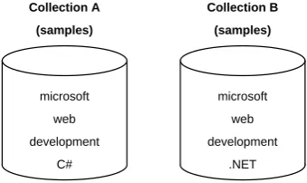
All resource description summaries that are constructed by random sam-pling techniques suer from the same problem. They are constructed from a small subset of documents from the collection they represent. Zipf's law [48, 29] states that given some corpus of natural language, the frequency of any word is inversely proportional to its rank in the frequency table. The most frequent word will occur approximately twice as often as the second most frequent word, which occurs twice as often as the fourth most frequent word, and so on. This means that most words in a collection occur only a few times and are thus not likely to be present in the small subset of retrieved sample documents. As a result, the content summary of a collection does not contain the majority of words that is present in the collection.
microsoft web development
C#
microsoft web development
.NET
Collection A
(samples)
Collection B
[image:12.595.236.406.425.526.2](samples)
Figure 1.2: Two incomplete sets of samples.
re-quests [43]. If we can assume that this hypothesis not only holds for docu-ments but also for collections of docudocu-ments, closely associated collections are also relevant to the same requests. Content summaries of topically similar collections can therefore complement each other.
1.5 Research questions
The focus of this research is the applicability of the cluster hypothesis to document collections instead of documents. We will research the possibility to improve collection selection methods using this hypothesis. The main research question is stated as follows:
Can the clustering of collections improve the performance of col-lection secol-lection methods for distributed web search?
What we want to prove is that the cluster hypothesis does not only hold for documents, but also for collections of documents. The cluster hypothesis is therefore rewritten as follows:
Closely associated collections tend to contain documents that are relevant to the same requests.
We further refer to this hypothesis as the collection cluster hypothesis.
In this thesis a number of research questions are answered. First of all we take a look at previous work on collection selection algorithms and choose an existing collection selection algorithm and use it for conducting experiments using collection clustering.
1. Which collection selection algorithm can be used in combination with collection clustering for this research?
This part of the research is purely based on literature about the subject. As a result we give an overview of the current state of the research in the eld, including a description of four well known collection selection algorithms.
2. How big is the problem of incomplete resource descriptions?
(a) What is the dierence in performance of collection selection be-tween scenarios where a full content summary is available and scenarios where content summaries are created using query based sampling techniques?
(b) What is the eect of the number of sampled documents from which the content summaries are constructed?
To answer these questions, we conduct collection selection experiments using the full collection data. We compare the results of these experiments to experiments conducted using query-based sampling with dierent numbers of samples. The results of these experiments show the relation between the number of samples and the performance of the collection selection algorithm.
In this research we setup a system for conducting clustering and collec-tion seleccollec-tion experiments. We need to simulate a distributed informacollec-tion retrieval environment. As test data the WT10G corpus is used, containing real-world data and queries. This corpus is split into collections so every collection can simulate a search engine as part of a distributed system. The retrieval experiments deliver ranked lists of collections. We need a way to measure the quality of the rankings in order to compare the results of the experiments. In traditional information retrieval, the most common mea-surements are recall and precision, but these meamea-surements can not be used directly for collection selection. This leads to the following research question:
3. How can the performance of dierent collection selection algorithms be measured and compared?
(a) How can the WT10G corpus be used for distributed information retrieval experiments?
(b) What are the most suitable measurements that can be used to com-pare collection selection algorithms?
If the test results of the modied algorithms show a signicant improve-ment over the original algorithms, we will assume that this positive eect is caused by the application of the cluster hypothesis. This would show that the cluster hypothesis is valid for collection selection in distributed search engines.
4. What is the best technique for collection clustering?
Two widely used cluster algorithms are the k-means algorithm and the bisecting k-means algorithm. We will conduct experiments using both al-gorithms and dierent parameters to determine which algorithm performs best.
The focus of this research is the use of collection clustering for collection selection. We will conduct experiments to evaluate the eects of clustering on collection selection. From the results we will be able to answer the following question:
5. What are the eects of clustering on the collection selection perfor-mance?
1.6 Thesis outline
Chapter 2
Literature
This chapter gives an overview of the relevant literature on the topics related to the research described in this thesis. We start by explaining Zipf's law and describing query-based sampling. This gives more insight in the cause of the problem of incomplete collection descriptions. Next, we describe the cluster hypothesis which is the theory on which our solution is based. In section 2.4 we discuss a number of collection selection algorithms. None of these algo-rithms use clustering to improve their performance. Section 2.5 discusses the k-means and bisecting k-means clustering algorithms. Section 2.6 describes some work that uses clustering to improve the quality of retrieval systems.
2.1 Zipf's law
Zipf's law [48, 29] states that given some natural language corpus, the fre-quency of any word is inversely proportional to its rank in the frefre-quency table. Simply said, many words occur very few times and a few words occur very often.
The most frequent word will occur approximately twice as often as the second most frequent word, which will occur approximately twice as much as
the fourth word, and so on. For example, in the British National Corpus1,
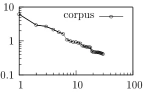
the most frequent word is `the' which accounts for slightly over 6% of all word occurrences, the word `of' accounts for almost 3% and the third most occurring word `and' accounts for 2.7% of all words. Only 157 dierent words are needed to account for half the corpus. A graph that shows the word frequencies of the corpus is shown in Figure 2.1. Figure 2.2 shows the same data, but plotted on logarithmic axes. This graph shows an almost straight line which indicates a power function.
Zipf found that this distribution can be described by the functionf(r) =
C
rα, where C is the coecient of proportionality, r is the word rank and
α is the exponent of the power law which typically has a value close to 1.
0 1 2 3 4 5 6 7
0 5 10 15 20 25 30
corpus b
bbb
bbbbbbbbbbbbbbbbbbbbbbbbbb
b
Figure 2.1: Word frequencies of the top 30 words from the British Na-tional Corpus.
0.1 1 10
1 10 100
corpus b
b b b bb
bbbbbbbbbbbbbbbbbbbbbbbb
[image:18.595.350.493.129.223.2]b
Figure 2.2: The same graph but plotted on logarithmic axes.
This function is found to apply not only to English texts but also to spoken language and non-English and non-Latin languages [32].
2.2 Query-based sampling
Query-based sampling [5, 9, 8] can be used to construct collection descrip-tions for collecdescrip-tions that can not or will not cooperate, or can not be trusted. Query-based sampling uses only the most basic functions of a collection: the possibility to submit queries to a search interface and retrieve a set of docu-ments from the result set. Most query-based sampling methods are designed to give a uniform and unbiased sample of the documents in a collection. If the sample is uniform and unbiased, the resource descriptions resemble the resource descriptions that would have been constructed if they were created from the full data collection. At the same time we want to minimize the costs of constructing these collection descriptions by keeping the number of inter-actions with the search interface and the number of retrieved documents as low as possible. The most straightforward query-based sampling algorithm is outlined below.
1. Select a one-term query.
2. Submit the selected one-term query to the search interface.
3. Retrieve the topndocuments from the result set.
4. Update the resource description based on the content of the retrieved documents.
5. If the stopping criterion has not been reached, go to step 1.
term is chosen from an external resource like a dictionary or a previously created language model. In subsequent iterations the query terms can be chosen from the language model that is learned from the retrieved docu-ments. A random term can be selected, but statistics about the number of occurrences of the words may also be used. Prior research [41] shows that using the least frequent terms in a sample yields a better resource description than randomly chosen terms for large collections.
Query-based sampling suers from two types of biases. Query bias is a bias towards longer documents that are more likely to be retrieved for a given query. Ranking bias is caused by the fact that search engines give certain documents higher ranks and query-based sampling only retrieves documents
up to rank n[40].
Bar-Yossef and Gurevich [3] describe two methods that are not aected by these biases and guarantee to produce near-uniform samples from a collec-tion. The samples that are taken rst are biased, but receive a weight which represents the probability of the document being sampled. These weights are used to apply stochastic simulation methods on the samples and obtain uniform unbiased samples from the collection.
The work described above focuses on retrieving uniform and unbiased samples. This is necessary for making size and overlap estimations of search engines. The question is whether unbiased samples are needed for creat-ing useful resource descriptions. For describcreat-ing resources, biased samples may be more representative. Gravano et al. [15] describe a technique called focused query probing which creates a topic specic description. This ap-proach is eective in scenarios in which resources contain topic specic and homogeneous content.
2.3 Cluster hypothesis
The cluster hypothesis is based on the idea that if a document is relevant to a given query, then similar documents will also be relevant to this query. This was formulated by Van Rijsbergen [43] as:
Closely associated documents tend to be relevant to the same re-quests.
If similar documents are grouped into clusters, then one of these clusters will contain the documents that are relevant to a query and the retrieval of the relevant documents is reduced to the identication of this cluster. This type of information retrieval is called cluster-based retrieval.
could be improved, but also the eectiveness. The reason for this is that cluster-based search takes into account the relationship between documents.
2.4 Collection selection algorithms
The purpose of collection selection is to select those collections that contain documents that are relevant to a user's query. Many collection selection algorithms have been proposed in literature. This section describes four well known collection selection algorithms that are based on dierent methods. From these algorithms we choose to use CORI for the experiments in this research.
2.4.1 GlOSS
GlOSS (Glossary-of-Servers Server) [13, 14] is one of the rst and well studied database selection algorithms. The original version of GlOSS was based on the rather primitive Boolean model for document retrieval. A generalized and more powerful version named gGlOSS was presented which is based on the vector-space retrieval model.
gGlOSS represents each collection ci by 2 vectors that contain the
fol-lowing values:
1. Document frequencyfij: the number of documents in collectionci that
contain termtj.
2. The sum of the weights wij of term tj over all documents inci. The
weight of a term tj in a document d is typically a function of the
number of times thattj appears indand the number of documents in
the collection that containtj.
gGlOSS denes the ideal rankingIdeal(l)as the ranking of the collections
according to their goodness. The goodness of a collectionc with respect to
queryq at threshold lis dened as
Goodness(l, q, c) = X
d∈{c|sim(q,d)>l}
sim(q, d) (2.1)
where sim(q, d) is a similarity function which calculates the similarity
between a queryq and a documentd.
Because the information that gGlOSS keeps about each collection is in-complete, assumptions are made about the distribution of the terms and their weights across the documents in the collection. An estimation of the
Ideal(l) rank is made using these assumptions. Two functions M ax(l) and
To derive M ax(l), gGlOSS assumes that if two words occur in a user query, then these words will appear in the collection document with the highest possible correlation. This means that if a query contains two terms
t1 andt2 that occur in respectivelyfi1andfi2 documents andfi1≤fi2, it is
assumed that every document in collection ci that containst1 also contains
t2.
A disjoint scenario is estimated bySum(l), where it is assumed that two
terms that appear in a user query do not both appear in the same document.
This means that the set of documents in ci that containst1 is disjoint with
the set of documents inci that containst2, if t16=t2.
2.4.2 Cue Validity Variance
The Cue Validity Variance method (CVV) [47] compares the variance of the cue validity of the query terms across all collections. The cue validity of term
t for collection ci measures the degree to which term t distinguishes
docu-ments inci from documents in other collections. CVV uses only document
frequency data to produce the rankings. The cue validity can be calculated using the function
CVij =
DFij
Ni
DFij
Ni +
P|C|
k6=iDFkj
P|C|
k6=iNk
(2.2)
where Ni is the number of documents in ci and |C| is the number of
collections in the system.
The cue validity variance CV Vj is the variance of the cue validities for
all collections with respect to tj. It can be used to measure the usefulness
of a query term for distinguishing one collection from another. The larger the variance is the more useful the term is to dierentiate collections. The collections are ranked based on a goodness score. Given a set of collections
C, the goodness of a collectionci∈C with respect to queryq withM terms
is dened as
Goodness(c, q) =
M
X
j=1
CV Vj ·DFij (2.3)
whereDFij is the document frequency of termj in collectionci. CV Vj is
the variance ofCVj which is the cue validity of term j across all collections.
2.4.3 CORI
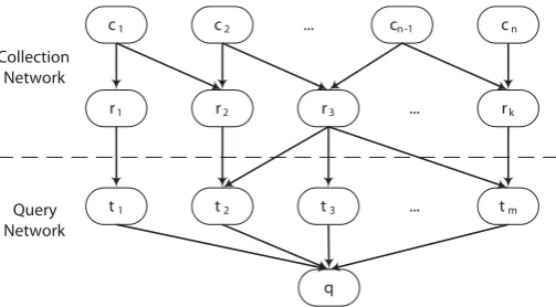
CORI [10] is an algorithm that takes a probabilistic approach to collection selection by using Bayesian inference networks [42]. These networks are directed acyclic graphs (DAGs). Figure 2.3 shows an example of an inference network that contains of four types of nodes. The nodes are connected by
edges, where an edge pointing from node p to node q is weighted with the
probabilityP(q|p)that q impliesp.
c1 c2 Collection
Network
Query Network
cn-1 cn
...
r1 r2 r3 ... rk
t1 t2 t3 ... tm
[image:22.595.195.447.265.404.2]q
Figure 2.3: Example of an inference network.
The leaf nodes cn are the collection nodes and correspond to the event
that a collection is observed. There is a collection node present for every
collection in the corpus. The representation nodes rk correspond to the
terms in the corpus. The collection nodes and representation nodes together form the collection network, which is built once for a corpus and does not change during query processing. The probabilities in this network are based
on collection statistics. CORI uses document frequencies (df) and inverse
collection frequencies (icf), that are calculated analogously to the common
tf and idf values. This is possible because a collection is treated as a bag
of words, just as a document is treated as a bag of words for calculatingtf
andidf. df is the number of documents containing a given term, icf is the
number of collections containing the term.
The query network contains a single query node q which represents the
user's query. The query nodestm correspond to the terms in the query. The
query network is built for each query and is modied during query processing.
The collection ranking score for queryq is the sum of the beliefsp(tm|ci)
in collection ci due to observing term tm ∈q. This belief can be calculated
p(tm|ci) =db+ (1−db)·T ·I (2.4)
T =dr+ (1−dr)·
log(df+ 0.5)
log(max_df + 1.0) (2.5)
I = log( |C|+0.5
cf )
log(|C|+ 1.0) (2.6)
where
df is the number of documents inci containingtm.
max_df is the number of documents containing the most
frequent term incci.
|C| is the number of collections.
cf is the number of collections containing termtm.
dr is the minimum term frequency component when
termtmoccurs in collectionci. The default value
is 0.4.
db is the minimum belief component when termtm
occurs in collectionci. The default value is 0.4.
The belief values are normalized to be between 0 and 1.
2.4.4 Indri
The retrieval model implemented in Indri [28, 27] uses a combination of the language model [31] and inference network approaches. Although it was not developed for collection selection it is possible to use it for that purpose by combining all documents of a collection into one single document [33]. A language model is constructed from every document in a collection. Given a
queryq, for every document the likeliness is estimated that the document's
language model would generate the query q. Indri uses language modeling
estimates rather thandf·icfestimates for calculating the beliefs of the nodes
in the inference network.
Instead of using Equation 2.4 for estimating the beliefs, Indri uses a probability based on the language model. This is probability is calculated by the equation
P(r|D) = tfr,D+αr
|D|+αr+βr (2.7)
This is the belief at representation nodergiven a documentD(in
collec-tionC). In this equation, αr and βr are smoothing parameters. Smoothing
it in collection C. The following values for the smoothing parameters are
used by default [27]:
αr=µ·P(r|C) (2.8)
βr=µ·(1−P(r|C)) (2.9)
whereµ is a tunable smoothing parameter which has a default value of
2500. Equation 2.7 can now be rewritten as
P(r|D) = tfr,D+µ·P(r|C)
|D|+µ (2.10)
Indri provides a query language that can express complex concepts. De-tails on this query language can be found in [39].
2.4.5 Discussion
Prior research gives an overview of the performance of the collection selection algorithm described above. CORI proves to be one of the most consistently eective algorithms in various situations [30, 12]. One known weakness in this algorithm is that the results are worse in environments that contain both very small and very large databases [35]. CVV can be very accurate when used with complete resource descriptions, but the performance drops when query-based sampling is used [11].
Indri is a fairly new algorithm compared to the other mentioned rithms. Not much research on comparing the performance to other algo-rithms has been conducted yet. There is research that shows promising results for specic retrieval tasks [46, 2], but the results are not consistently good.
We choose to use CORI as the collection selection in this research because of its performance, but also because it is implemented in the freely available Lemur toolkit for language modeling and information retrieval. It can be used out-of-the box which means we do not need to implement the algorithm ourselves.
2.5 Clustering
The objective of document clustering is to group documents together that share the same implicit topic. At the same time, the dierent clusters should have dierent topics. There are various motivations within the eld of in-formation retrieval to perform clustering. Using document clustering it is possible to automatically create browsable taxonomies like the Yahoo
Di-rectory2. Taxonomies are usually manually created, which takes a lot of
eort to keep them up-to-date. A dierent goal of document clustering is to improve the eciency of information retrieval systems. Searching clusters of documents together instead of all documents separately can decrease the number of calculations and therefore increase the speed of the search opera-tion. Clustering can also be used to show the query results grouped by topic. This can give users a better overview of the dierent documents that were found and the relationships among them.
A good document clustering algorithm produces clusters that meet the following criteria:
• The intra-cluster similarity is high, which means documents in the
same cluster are similar.
• The inter-cluster similarity is low, which means documents in dierent
clusters are dissimilar.
2.5.1 Clustering types
There are two types of clustering methods: hierarchical and partitional meth-ods. Hierarchical clustering methods generate trees of clusters, so called den-dograms. The root of such a tree is a cluster that contains all documents and the leaves are individual documents. Hierarchical clustering algorithms can be either divisive where the dendogram is created by starting with one cluster containing all documents and recursively splitting the clusters into smaller ones, or agglomerative where at the start every document is consid-ered a cluster which is recursively merged into a bigger cluster. Partitional clustering methods on the other hand create a one-level partitioning of the documents. This is typically done by selecting a number of initial clusters and assigning all documents to the closest cluster based on some measure of similarity.
2.5.2 K-means algorithm
The k-means algorithm [24, 26] is one of the most widely used clustering algorithms. It is a partitional algorithm that is based on the idea that a cen-troid can represent a cluster. Clustering is seen as a optimization problem in which an assignment of data vectors to clusters is desired, such that the sum of the similarities between the vectors and their cluster centroids is
opti-mized. The document set containingndocuments is denoted byd1, d2, ..., dn.
The objective is choose the number of clusters k and assign the documents
to these clustersCj in such a way that the function
k
X
j=1
X
di∈Cj
is either minimized or maximized, depending on the choice of the
sim-ilarity function sim(di,cbj). This similarity function gives a value for the
similarity between a document vector di and a cluster centroid cbj which is
a measure for the intra-cluster similarity. K-means does not take the inter-cluster similarity into account. Dierent similarity functions can be chosen, but most common is to use the Euclidean distance or cosine distance. The cluster centroid can be dened in dierent ways, but is often the median or
the mean point of the cluster. The mean point of a cluster Cj that consist
of the document setd1, d2, ..., dn is given by
b cj =
1
|Cj|
X
di∈Cj
di (2.12)
which is the vector obtained by averaging the weights of the various terms present in the cluster's documents.
Finding the best clustering, thus maximizing function 2.11, is know to be an NP-hard problem [26] and therefore a heuristic algorithm is generally used which gives an approximate solution. It maximizes the sum of the intra-cluster similarity values when an initial assignments of centroid is provided.
The number of clusters k is xed during the run of the algorithm and is
chosen based on the problem and domain.
1. Select k points as the initial centroids. These points are selected
ran-domly. A point is a vector representing a collection of documents or a single document.
2. Assign all points to the cluster with the closest centroid. Which is the closest centroid is determined by the similarity function.
3. Recompute the centroid of each cluster.
4. Repeat steps 2 and 3 until the centroids don't change.
The resulting clustering depends on the choice of the initial centroids. There is no guarantee that it will converge to a global optimum. It is common to run the algorithm multiple times with dierent initial centroids and select from the results the best clustering according to function 2.11.
Because the initial centroids are chosen in the rst step, the number of
collections, represented by k, must be specied prior to application. The
choice ofktherefore highly inuences the results and must be carefully
cho-sen. Another eect of choosing the centroids in the rst step is that the variation in size of the resulting clusters may be large. An initial centroid which is central in the vector space may grow large, while an outlier may become a very small cluster.
thousand of clusters, the eciency decreases and the complexity approaches
O(n2) wherenis the number of documents [44].
2.5.3 Bisecting k-means algorithm
Bisecting means [38, 23] creates a hierarchical cluster tree using the k-means algorithm. It has two major advantages over the k-k-means algorithm. First, the complexity of the algorithm is linear to the number of documents,
thus O(n). Second, the number of clusters that is produced does not
neces-sarily need to be known beforehand, as we will describe later in this section. It is an agglomerative method so initially the whole collection set is con-sidered one cluster. Recursively, a cluster is selected and split into two clus-ters using the k-means algorithm until a stopping criterion has been reached. The algorithm typically stops when the desired number of clusters is reached.
1. Select a cluster to split. There are several ways to do this. Most common is to select the largest cluster, the cluster with the least overall similarity or a combination of cluster size and similarity.
2. Divide the cluster into two clusters using the k-means algorithm. This
means executing the algorithm usingk= 2.
3. Repeat step 2 for a xed number of times. Select the split with the highest overall similarity. The results of the k-means algorithm are dependent on the randomly selected initial clusters. By repeating this a number of times the quality of the resulting clusters can be improved.
4. Repeat steps 1-3 until the stopping criterion is reached, typically when a maximum number of clusters is created.
The complexity of the bisecting k-means clustering is linear to the number of documents [38]. This makes it more ecient than the k-means algorithm when the number of clusters is large. This is caused by the fact that there is no need to calculate the distance of every document to the centroid of each cluster since we consider only two centroids in the bisecting step.
Specifying cluster sizes The number of clusters and the sizes of the clusters are dependent on the stopping criterion in step 4. We can control the number of clusters that should be produced by stopping the algorithm when a certain number of clusters has been reached. We also have more control of the number of documents contained in each cluster. When a
cluster has reached a size smaller than a given maximum size smax we can
decide not to split it any further and choose another cluster to split or stop the algorithm. We also want to be able to specify a minimum cluster size
smaller thansmin, we discard the split and create another split for clusterc.
This requires thatsmax≥smin·2−1.
New collections can be added to an existing clustering by assigning them to the cluster with the closest centroid. We must keep in mind that the
clusters do not grow bigger than smax. When this happens, we split this
cluster into two clusters.
2.6 Cluster-based retrieval
Some research on cluster-based retrieval has already been performed. Xu and Croft [45] describe three methods for optimization of distributed infor-mation retrieval by clustering the resources. Using the rst two methods called global clustering and local clustering, the documents are physically partitioned into collections. This requires besides a global coordinating sys-tem the cooperation of the collections. The third method, multiple-topic representation, does not require physical partitioning and avoids the cost of re-indexing. Each subsystem summarizes its collection as a number of topic models. With this method, a collection corresponds to several topics. The INQUERY retrieval system [7] is used for indexing and searching collections. The steps to search a set of a distributed collections for a query are (1) rank the collections against the query, (2) retrieve 30 documents from each of the best n collections, (3) merge the retrieval results based on the document scores.
SETS [4] is an algorithm for ecient distributed search in P2P networks. Participating sites are categorized by topic. Topically focused sites are con-nected by short-distance links and clustered into segments. These segments are connected by long-distance links. Queries are sent only to the topically closest segments.
The algorithm described in [34] automatically categorizes specialty search engines into a hierarchical structure based on the textual content of the
documents. The taxonomy from the DMOZ Open Directory Project3 is used
during the research. Collections are classied into taxonomy categories by using probe queries. This is very similar to the work described by Ipeirotis at al. [20, 18]. First a hierarchical classication scheme or taxonomy is dened. For each category in this taxonomy a number of probe queries are generated. These are queries that return a set of results that is relevant to the category.
The queryJ ordan AN D Bulls for example will retrieve mostly documents
in the sports category. Instead of retrieving the actual documents, only the number of results is counted. From the number of matches for each probe query it is possible to make an estimation about the topics covered by a collection and categorize the collection in the taxonomy. In more recent work Ipeirotis at al. [19] describe an algorithm for collection selection for a
given query. From the top of the hierarchy at each level the best category is selected using existing algorithms as GlOSS or CORI. This process proceeds recursively until the number of collections under the selected category drops below a certain value.
2.7 Summary
This chapter gave an overview of the relevant literature about the topics related to the research described in this thesis. A explanation of Zipf's law is given, as well as a description of query-based sampling to give some background information on the cause of the problem of the incompleteness of the collection descriptions.
Four collection selection algorithms are discussed. We chose to use CORI for the experiments in this research because of its performance and because it is included in the Lemur toolkit for language modelling and information retrieval.
Chapter 3
Research
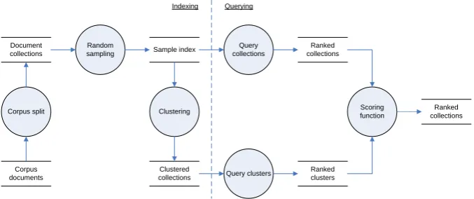
In this research, we use a prototype of a distributed information retrieval system. An overview of the system is shown in Figure 3.1. The system is divided into two parts. The indexing on the left side is initiated by the server and produces two indexes that are needed to perform the querying. The querying, shown on the right, is initiated by the users. It involves selecting relevant collections from the index and ranking them according to their supposed relevance to the user's query. This chapter will describe in detail how the dierent parts of the system are implemented. Further, it will describe how the evaluation of the system is performed.
Document collections
Random
sampling Sample index
Clustering
Clustered collections
Query collections
Query clusters
Ranked collections
Ranked clusters
Scoring function
Ranked collections
Indexing Querying
[image:31.595.103.442.436.578.2]Corpus documents Corpus split
Figure 3.1: Experimental setup.
3.1 The WT10g corpus
documents were removed, as well as duplicate and redundant data. Details about the construction of the WT10g corpus can be found in [1]. Some
statistics on the WT10g corpus as taken from the TREC website1 are:
• 1,692,096 documents
• 11,680 servers
• an average of 144 documents per server
• a minimum of 5 documents per server
A number of measurements on the WT10g corpus is performed by Sobo-ro [37]. FSobo-rom this measurements the conclusion is drawn that the corpus retains the properties of the web, and is therefore a good representation of the web for research purposes.
There are two sets of topics with relevance judgements that can be used with the WT10g corpus. Topics 451-500 include a number of misspelled words, topics 501-550 do not. The relevance judgements tell whether a doc-ument is considered to be relevant to a topic or not. These relevance judge-ments are made by humans and classify docujudge-ments as irrelevant, relevant or highly relevant.
Splitting the corpus The WT10g corpus was not created for distributed information retrieval. Compared to previous TREC corpora, WT10g has better support for distributed information retrieval. However, it is not pos-sible to use it for distributed information retrieval experiments without any preprocessing. In order to represent a distributed environment consisting of a lot of dierent search engines, the corpus is split based on the server IP address. By doing so, we create 11,512 separate data collections. This is a little less than the 11,680 servers that are present in the WT10g corpus, which means that a few servers share the same IP address.
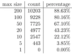
We counted the number of documents in each collection. The smallest collection contains 5 documents and the largest collection contains 26,505 documents. The average collection size is 147. This is a little more than the 144 documents per server in the corpus, which is again caused by the fact that we have a little less collections than there are servers in the corpus. Table 3.1 shows the number of collections with a given maximum size. The collections are fairly small, only 11.37% of the collections contains more than 200 documents.
A split created this way is representative for a scenario where small search engines index single websites. In this scenario, there is no overlap between the indexes of the search engines. Documents are present in just one index. We
Table 3.1: Collection sizes
max size count percentage
200 10203 88.63%
100 9228 80.16%
50 7725 67.10%
20 4977 43.23%
10 2547 22.12%
5 443 3.85%
1 0 0.00%
expect that there will be coherence in the topics of the documents contained by these collections. This means we expect that two documents on a single server are more likely to share the same topic than two documents that reside on dierent servers.
Documents and collections A collection contains all documents that originate from a server with the same IP address. The data from these documents is merged into a single le and assigned a unique identier for the collection. This is possible because CORI treats collections as bags of words, as if they were large single documents. No statistics are used about the individual documents in the collections.
3.2 Random sampling
In practice all random sampling techniques are biased. In this research we do not want this to aect our results. It is also not necessary to use a technique like query based sampling, because we have the full corpus at our disposal. By randomly selecting documents from a known collection, we simulate the perfectly random sampling method. The selected samples are a subset of the full collection data and are indexed as the sample index.
Creating indexes In order to evaluate the eect of the number of sam-ples used in the random sampling procedure, we create dierent indexes for dierent amounts of samples. From every collection in the corpus, we
taken randomly selected documents and store these as a partial collection.
This way a new index can be constructed where every collection contains
at most n documents. If a collection contains less than or exactly n
doc-uments, this means the full collection will be retrieved. We create indexes
for n ∈ {1,5,10,20,50,100,200}. For comparison, an index is created that
3.3 Clustering
After the random sampling indexes have been created we cluster the sampled collections. We use both the k-means and the bisecting k-means algorithm. When the k-means algorithm is used we have to give the number of clusters that is to be produced as a parameter. Using bisecting k-means we specify the upper and lower bounds of the cluster sizes.
3.3.1 Reducing the calculations complexity
We make some compromises in the way we execute the clustering algorithm in order to reduce the number of calculations needed during the clustering process. These compromises are similar to those described in [44].
First of all, the feature vectors that represent the collections are reduced to the 25 most frequently occurring terms in the collection. Stop words are removed from the feature vectors rst. This highly reduces the number of calculations needed to calculate the distance between collections and cluster centroids.
Second, we reduce the number of iterations in the splitting step. In the original k-means algorithm all collections are reassigned to the closest centroid until the centroids do not change. It may take a long time before the clusters converge to a situation like that while the clusters do not change much. For the k-means algorithm we conduct experiments with dierent numbers of iterations to test the inuence of this on the collection selection results. For the bisecting k-means algorithm we limit the number of iterations to a maximum of three.
In the bisecting k-means algorithm, the splitting of the clusters is per-formed multiple times after which the best split is selected. This is done to reduce the eect of the random selection of the initial centroids during the execution of the k-means algorithm. We execute this step only two times to reduce the number of calculations.
3.3.2 K-means
Number of clusters The k-means algorithm requires a value for the
pa-rameterk, the number of clusters that is to be produced. We run collection
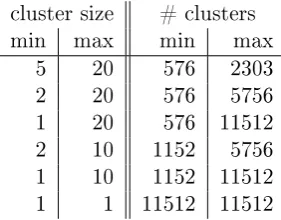
Table 3.2: Cluster sizes for bisecting k-means
cluster size # clusters
min max min max
5 20 576 2303
2 20 576 5756
1 20 576 11512
2 10 1152 5756
1 10 1152 11512
1 1 11512 11512
Cluster quality As explained in the previous section, one of the means to reduce the complexity of the calculations is to limit the number of iterations for reassigning the collections to the clusters. This aects the quality of the clusterings. The intra-cluster similarities of the clusters will be lower. We run experiments where the number of iterations is limited to 1, 5 and 25. We evaluate the eects of the number of clusters on the collection selection performance.
3.3.3 Bisecting k-means
We adjusted the bisecting k-means algorithm in such a way that it allows us to specify the sizes of the clusters that are produced by the algorithm. The size of the clusters may aect the performance of the nal collection selection step. In order to tell what the eects of the cluster sizes are, we produce a number of clusterings with dierent cluster sizes. Our implementation of the bisecting k-means algorithm does not allow us to dene the exact size of the clusters but we can set a minimum and maximum size. Clusters that have a size larger the the maximum size are split. If one of the clusters that is produced by splitting a larger cluster is smaller than the minimum size, the split is considered invalid and splitting is performed again until the sizes of both clusters are in the desired range. Setting a minimum size may favor clusters with a certain size over clusters with high intra-cluster similarity, which leads to clusterings with lower quality. For that reason we keep the minimum cluster size low.
3.3.4 Indexing clusters
All collections that are in a single cluster are merged together as a single collection. Since a collection is represented by CORI the same way as a document, a cluster is also represented as a document. This way it can be indexed by a general information retrieval system without any adjustments.
3.4 Ranking collections
Upon query time, the system generates a ranked list of collections that are relevant to the query. This list is created in three steps, that are visualized in the right part of Figure 3.1.
1. A ranked list is created by ranking the collections from the index where no clustering was applied. This assigns a ranking score to each indi-vidual collection.
2. The clusters are ranked using the index that contains the clustered data. Each cluster is assigned a ranking score.
3. A scoring function combines the scores from step 1 and step 2 to a combined score for each collection. The nal ranking is created by rearranging the collections based on the combined scores.
We use the CORI algorithm as it is implemented in the Lemur toolkit to perform the actual collection selection steps (1 and 2). Collections and clusters are indexed and queried as if they were documents.
For this research the scoring function is kept simple. It calculates the combined scores by adding the cluster scores and collection scores. Because both scores are calculated using CORI, no normalization is needed. Other scoring functions are possible, for example to let the cluster score account more to the combined score.
3.5 Evaluation
This section describes the metrics that are used for the evaluation of the test results. For the evaluation of the query results we use two metrics: recall and precision.
Collection merits The calculation of the recall and precision scores are based on relevance judgements. Relevance judgements are binary and tell whether a document is relevant or irrelevant to a query. The relevancy of a collection is given by the number of relevant documents contained by this collection. This number of relevant documents is called the merit of a collection.
Recall and precision In traditional information retrieval, precision and recall are the most widely used metrics for results evaluation. Similar metrics were dened for distributed information retrieval by Gravano et al. [13].
We know which documents are relevant to each query. From this infor-mation we calculate a merit score for each collection by simply counting the
number of relevant documents in that collection. The merit of collection ci
for queryq can be expressed as merit(q, ci).
In the ideal ranking, the collections with the highest merit score are
ranked rst. We use this ranking as our baseline ranking B. The merit
of the ith collection in this ranking is given by Bi = merit(q, cbi). For the
ranking under evaluation, the merit is given by Ei=merit(q, cei)
The recall is dened by Gravano et al. as
Rn=
Pn
i=1Ei
Pn
i=1Bi (3.1)
This recall is a measure of how much of the available merit in the top n
ranked collections has been accumulated by the ranking under evaluation. A slightly dierent recall measure was dened by French et al. [12] as
c Rn=
Pn
i=1Ei
Pn∗
i=1Bi
where
n∗=max(k) such thatBk 6= 0.
(3.2)
n∗ is the breakpoint between the relevant and non-relevant collections.
The denominator is the total merit of all collections that are relevant to the
query. The recall Rcn gives the percentage of the total merit that has been
Rn can be 1 from the beginning, when the ranking under evaluation is
equal to the ideal ranking, while Rcn will gradually increase to 1. This also
means that Rn can decrease asn increases. From the point where n=n∗,
the values forRn are equal toRcn. BecauseRcnis always increasing, it is the
most similar to the tradition recall metric.
Gravano et al. [13] also describe a precision metric that can be used in
collection selection scenarios. It gives the fraction of the collectionsrc with
a non-zero merit that occur in theT opnretrieved results. A higher precision
Pnis better because it reduces the number of database searches that will not
give any relevant results.
Pn=
|{rc∈T opn(S)|merit(q, rc)>0}|
n (3.3)
Signicance tests When two collection selection algorithms are compared and a dierence is found, it is still a question whether this dierence is signicant or not. Some algorithms may do better for certain queries but worse for others. Signicance test can be used to statistically prove that one algorithm performs truly better than another.
In information retrieval research, commonly used tests are the Student's paired t-test, the Wilcoxon signed rank test and the sign test. Smucker et al. [36] showed that the Wilcoxon and sign test have the potential to lead to false detections of signicance. We will use the Student's paired t-test.
We run the signicance test on two paired sets of results. These are the
recall or precision values per query for both algorithms after n collections
are retrieved. We assume that these sets of results are samples taken from normally distributed population. The null hypothesis is that there is no dierence between the two algorithms.
A signicance level is calculated from the paired result sets. This signif-icance level gives the probability that the results could have occurred under the null hypothesis. A high value means that there is a high probability that there is no dierence between the two algorithms. This signicance level is also known as the p-value. We dene that a p-value under the threshold of 0.05 disproves the null hypothesis. In this case we can say with a certainty of 95% that there is a dierence between the two algorithms and therefore
3.6 Summary
A setup was described for conducting collection selection experiments using clustering of collections. The experiments consist of the following steps:
1. Create a split of the WT10g corpus based on the IP address of the web server from where the documents were retrieved.
2. Perform random sampling of the corpus split. We do not use query-based sampling but take random samples from the full collections that are accessible.
3. Cluster the collections. We conduct experiments using the k-means and the bisecting k-means algorithm.
4. Run the queries and create ranked lists of collections.
Chapter 4
Results
This section gives an overview of the results of the conducted experiments. There are a few points of attention one must keep in mind before looking at the graphs in the following sections:
a) The recall and precision graphs show only the results for the rst 1,000 retrieved collections. It is highly unlikely that in practice more collections will be addressed for a query. The collections that are ranked at the top are considered to be the most important, which is why the horizontal axes are on logarithmic scale. The recall is calculated using Equation 3.1, for calculating the precision Equation 3.3 is used.
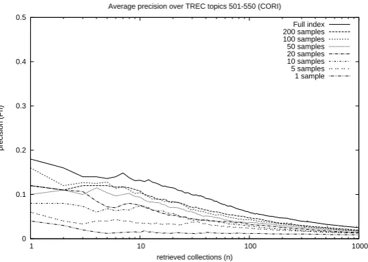
b) It is also important to notice that the vertical axis of the precision graphs ranges from 0 to 0.5 while the range is 0 to 1 for the recall graphs.
c) In the precision graphs, some lines seem to be missing. This happens when two lines are exactly the same so they overlap.
d) Only the graphs that are considered to be the most important are shown. More graphs can be found in the appendices.
4.1 Query-based sampling
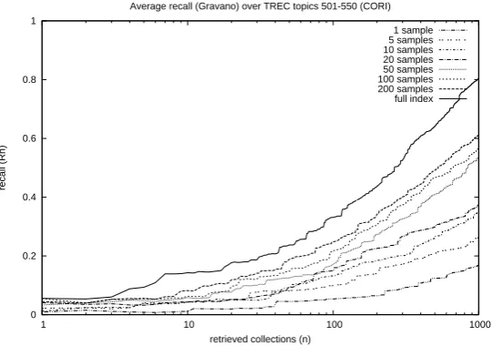
In order to measure the eects of query-based sampling with dierent num-bers of samples, retrieval experiments are run without using clustering. Fig-ure 4.1 shows the average recall over TREC topics 501-550 for the dierent number of samples. The graph clearly shows that on general the performance increases with the number of samples.
0 0.2 0.4 0.6 0.8 1
1 10 100 1000
recall (Rn)
retrieved collections (n)
Average recall (Gravano) over TREC topics 501-550 (CORI)
[image:42.595.183.454.127.317.2]1 sample 5 samples 10 samples 20 samples 50 samples 100 samples 200 samples full index
Figure 4.1: Average recall for dierent numbers of samples.
of samples is used. The explanation for this eect is the randomness of the samples that are taken. A smaller set of samples may contain documents that make a collection give a high rank while a larger set of samples may contain only documents that make the collection seem irrelevant and give it a low score. This eect is visible in the graphs because the random sampling phase was executed only once for every number of samples.
Although the full collection was indexed for more than 88% of the col-lections when 200 samples are taken, the dierence in performance with the situation where the full index was used for all collections is still signicant for both recall and precision at most points in the graphs. The exact recall and precision values and details about the signicance of the results can be found in Tables D.1 and D.2 in Appendix D.
The results of these experiments are used as the baseline for the exper-iments that use clustering of collections. They were produced in a general distributed information retrieval setting. The lines in the graphs can also be found in the result graphs of the experiments that where based on clustering of collections, where they were added for comparison.
4.2 Cluster sizes and the number of clusters
0 0.1 0.2 0.3 0.4 0.5
1 10 100 1000
precision (Pn)
retrieved collections (n)
Average precision over TREC topics 501-550 (CORI)
[image:43.595.136.405.165.356.2]Full index 200 samples 100 samples 50 samples 20 samples 10 samples 5 samples 1 sample
Figure 4.2: Average precision for dierent numbers of samples.
20 25 30 35 40 45 50 e nt age of clust ers
Percentage of clusters per cluster size
384 767 1535 3835 0 5 10 15 20 25 30 35 40 45 50
1 2 3 4 5 6 7 8 9 10 11 12 13 14 15 16 17 18 19 20 >20
Pe rcent a ge of clust e rs Cluster size Percentage of clusters per cluster size
384 767 1535 3835
[image:43.595.134.413.480.649.2]relatively many clusters that contain only a single collection.
In our implementation of the bisecting k-means algorithm we dene the size of the clusters that is produced. There are no hard cluster sizes used, but upper and lower bounds. Within these boundaries, the sizes of the clusters that are created may vary. The distribution of the cluster sizes for the clusterings based on 200 samples is plotted in Figure 4.4. In this gure, the y-axis shows the absolute number of clusters. In all 5 cases the number of clusters which size is equal to the minimum size is relatively large.
200 250 300 350 400 450 500 m b er o f cl u s ter s
Number of clusters per cluster size
1-10 1-20 2-10 2-20 5-20 0 50 100 150 200 250 300 350 400 450 500
1 2 3 4 5 6 7 8 9 10 11 12 13 14 15 16 17 18 19 20
Nu m b er o f cl u s ter s Cluster size Number of clusters per cluster size
[image:44.595.181.463.248.413.2]1-10 1-20 2-10 2-20 5-20
Figure 4.4: Number of clusters per cluster size (Bisecting k-means, 200 samples).
Collections that form a cluster by themselves can also be so called out-liers. These collections are not similar to any other collections and therefore not grouped into a cluster with other collections.
The fact that there are relatively many small clusters might have a neg-ative eect on the retrieval performance. A clustering with many small clusters is very similar to the situation where no clustering is performed at all.
Number of clusters for k-means In Figure 4.5 we compare the recall
of the collection selection experiments using dierent numbers for k, the
number of clusters that is produced by the k-means algorithm. The solid line is the graph of the experiment without using clustering. For the rst 10 retrieved collections, we see that the recall is higher when clustering is used for all numbers of clusters. At this interval, the clusterings with 767 and 1,535 clusters perform best, while the clustering with 3,837 clusters follows almost the same line as the baseline graph without clustering. After 50 retrieved collections we see that a larger number of clusters leads to a higher recall.
0 0.2 0.4 0.6 0.8 1
1 10 100 1000
recall (Rn)
retrieved collections (n)
Average recall (Gravano) over TREC topics 501-550 (CORI)
[image:45.595.135.404.452.646.2]3837 clusters 1535 clusters 767 clusters 384 clusters No clustering
Figure 4.5: Average recall for dierent numbers of clusters (K-means, 200 samples, 5 iterations).
0 0.1 0.2 0.3 0.4 0.5
1 10 100 1000
precision (Pn)
retrieved collections (n)
Average precision over TREC topics 501-550 (CORI)
3837 clusters 1535 clusters 767 clusters 384 clusters No clustering
tinction between the dierent clusterings is less clear then for the recall graphs. For the rst 10 retrieved collections the precision is higher than the baseline when clustering is used, except for the experiment with 3,837 clusters which only shows a small improvement for the rst 4 retrieved col-lections. The clustering with 767 clusters has the best performance. The precision of the clustering with 3,837 clusters is close to the precision of the baseline so clustering with that many clusters has only a small inuence on the precision.
0 0.2 0.4 0.6 0.8 1
1 10 100 1000
recall (Rn)
retrieved collections (n)
Average recall (Gravano) over TREC topics 501-550 (CORI)
200 samples (5-20) 200 samples (2-20) 200 samples (1-20) 200 samples (2-10) 200 samples (1-10) 200 samples (1)
Figure 4.7: Average recall for dierent cluster sizes (Bisecting k-means, 200 sam-ples).
Cluster sizes for bisecting k-means Figure 4.7 shows the recall of the experiments using clustering using bisecting k-means for 200 samples. The dierent graphs show the recall values for dierent boundaries of the cluster sizes. The solid line shows the recall when no clustering is used. This is the same graph as in Figure 4.1 and is used as the baseline.
The results show an increase in performance for the rst 10 retrieved collections for the retrieval experiments where clustering is used. After 20 retrieved collections the recall for all cluster sizes drops below the baseline graph. The recall graphs for the dierent cluster sizes are close to each other and cross at some points. From this gure it is not possible to say which cluster size has the best performance.
0 0.1 0.2 0.3 0.4 0.5
1 10 100 1000
precision (Pn)
retrieved collections (n)
Average precision over TREC topics 501-550 (CORI)
200 samples (5-20) 200 samples (2-20) 200 samples (1-20) 200 samples (2-10) 200 samples (1-10) 200 samples (1)
Figure 4.8: Average precision for dierent cluster sizes (Bisecting k-means, 200 samples).
cluster sizes cross a few times, so also from this gure it is not possible to determine a cluster size with the best performance.
For bisecting k-means there is no cluster size that produces consistently better results than other cluster sizes. We therefore conclude that the cluster size has no or only a small inuence on the retrieval performance, at least for clusters with a minimum size of 1 and a maximum size of 20 collections.
4.3 Cluster quality
In section 3.3.1 we discussed some compromises we made to reduce the com-plexity of the calculations of the cluster algorithms. One of these compro-mises is a limit to the number of iterations for the k-means algorithm. We conducted experiments with dierent numbers of iterations to evaluate the eects of these compromises. Figure 4.9 shows the recall for the collection selection experiments using k-means clustering with dierent numbers of it-erations.
For the experiments with 100 samples as well as the experiments with 200 samples we see that the results are just slightly dierent for dierent numbers of iterations. At some points in the graphs we see that the recall for the experiments with just one iteration is a little worse.
0 0.2 0.4 0.6 0.8 1
1 10 100 1000
recall (Rn)
retrieved collections (n)
Average recall (Gravano) over TREC topics 501-550 (CORI)
K-means, 200 samples, 767 clusters (25 iter.) K-means, 200 samples, 767 clusters (5 iter.) K-means, 200 samples, 767 clusters (1 iter.) K-means, 100 samples, 767 clusters (25 iter.) K-means, 100 samples, 767 clusters (5 iter.) K-means, 100 samples, 767 clusters (1 iter.)
Figure 4.9: Average recall using k-means with dierent numbers of iterations.
cluster algorithm increases linearly with the number of iterations and we want to keep the necessary resources low, we use 5 iterations for the rest of the experiments. From these graphs we conclude that this will hardly aect the results.
4.4 Comparing cluster algorithms
This section compares the results of the k-means algorithm, the bisecting k-means algorithm and the baseline without clustering. The k-means graphs show the results of the experiment with 767 clusters and 5 iterations. We chose this number of clusters because it has the best performance as shown in the previous section. For the bisecting k-means algorithm there is no cluster size that performs best, so we include the graphs for the two cluster sizes that dier the most: 1-10 and 5-20.
The recall graphs for 200 samples are show in Figure 4.11. All graphs show an improvement in performance over the baseline for the rst 10 re-trieved collections. The recall improves signicantly and increases 96% to 181% between 2 and 6 retrieved collections for all algorithms as can be seen in more detail in Table D.3 in Appendix D. The dierences between the cluster algorithms is small. The recall graphs for 100 samples that can be found in Appendix C show less improvement, but improvement is still visible for the rst 10 retrieved collections.
0 0.1 0.2 0.3 0.4 0.5
1 10 100 1000
precision (Pn)
retrieved collections (n)
Average precision over TREC topics 501-550 (CORI)
K-means, 200 samples, 767 clusters (25 iter.) K-means, 200 samples, 767 clusters (5 iter.) K-means, 200 samples, 767 clusters (1 iter.) K-means, 100 samples, 767 clusters (25 iter.) K-means, 100 samples, 767 clusters (5 iter.) K-means, 100 samples, 767 clusters (1 iter.)
Figure 4.10: Average precision using k-means with dierent numbers of iterations.
0 0.2 0.4 0.6 0.8 1
1 10 100 1000
recall (Rn)
retrieved collections (n)
Average recall (Gravano) over TREC topics 501-550 (CORI)
K-means, 767 clusters Bisecting k-means, 5-20 Bisecting k-means, 1-10 No clustering
0 0.1 0.2 0.3 0.4 0.5
1 10 100 1000
precision (Pn)
retrieved collections (n)
Average precision over TREC topics 501-550 (CORI)
K-means, 767 clusters Bisecting k-means, 5-20 Bisecting k-means, 1-10 No clustering
Figure 4.12: Average precision using clustering (200 samples).
quickly when more collections are retrieved. When more than 5 collections are retrieved, the precision score is lower than for the situation without clustering. The bisecting k-means clustering with cluster sizes in the range from 1 to 20 has a low precision for the rst retrieved collection, but the precision increases for the next few collections. The k-means algorithm has a high precision and it does not increase or decrease as much as the precision for the bisecting k-means algorithm. The results for the k-means algorithm are more stable. For all algorithms there is only signicant improvement in precision for the rst 4 retrieved collections.
4.5 Query sets
0 0.1 0.2 0.3 0.4 0.5
1 10 100 1000
precision (Pn)
retrieved collections (n)
Average precision over TREC topics 451-500 (CORI)
[image:51.595.135.407.126.316.2]Full index 200 samples 100 samples 50 samples 20 samples 10 samples 5 samples 1 sample
Figure 4.13: Average precision for