Loop inflection-point inflation
Konstantinos Dimopoulos,1 Charlotte Owen,1 and Antonio Racioppi2
1
Consortium for Fundamental Physics, Physics Department, Lancaster University, Lancaster LA1 4YB, United Kingdom
2National Institute of Chemical Physics and Biophysics, R¨avala 10, 10143 Tallinn, Estonia (Dated: July 5, 2018)
A novel inflection-point inflation model is analysed. The model considers a massless scalar field, whose self-coupling’s running is stabilised by a non-renormalisable operator. The running is con-trolled by a fermion loop. We find that successful inflation is possible for a natural value of the Yukawa coupling y'4×10⁻⁴. The necessary fine-tuning is only ∼10−6, which improves on the typical tuning of inflection-point inflation models, such as MSSM inflation. The model predicts a spectral index within the 1-σ bound of the latest CMB observations, with a very small negative running, and negligible tensors (r∼10−(9−10)). These results are largely independent of the order of the stabilising non-renormalisable operator.
INTRODUCTION
Cosmic inflation is an organic part of concordance cos-mology. With a single stroke inflation addresses the fine-tuning problems of the hot big bang; namely the horizon and flatness problems and also produces the primordial cur-vature perturbation, which seeds structure formation and is in excellent agreement with CMB observations [1]. Ac-cording to the inflationary paradigm, the Universe under-goes inflation when dominated by the potential density of a scalar field, called the inflaton. However, the identity of the inflaton is as yet unknown.
The latest CMB observations suggest that the scalar po-tential of the inflaton features an inflationary plateau (e.g. see Ref [2]). Numerous mechanisms have been put forward to generate such a plateau, involving exotic constructions in the context of elaborate, beyond-the-standard-model theo-ries, such as superstrings. One such example is inflection-point inflation, where the inflationary plateau is due to the interplay of opposing contributions in the scalar potential, which (almost) cancel each other out generating a step on the otherwise steep potential wall. The original model was called A-term inflation, because it employed the A-term of a supersymmetric theory [3,4], or MSSM inflation, because it considered a flat direction in MSSM [5] as the inflaton. However, other models of inflection-point inflation have also been constructed [6,7]. Most of these also consider an elab-orate setup in the context of supersymmetry, string theory or other extensions of the Standard Model.
However, an advantage of the idea of inflation is that it does not have to rely on exotic physics, in contrast to alternatives like the ekpyrotic scenario [8] or string gas cosmology [9]. Indeed, inflation may be realised simply within field theory in curved spacetime. It is also possible to achieve inflection-point inflation in this way. In this pa-per we explore such a possibility, where we exploit the loop corrections to the inflaton potential to generate the step-like plateau. This is similar to the works in Ref. [7]. How-ever, in Ref. [7] the authors consider a rather complicated running of the inflaton self-coupling, where many particles
are contributing to it. We consider a simpler setup. In previous works care was taken so that loop corrections do not spoil the stability of the potential [10]. In contrast, here we consider a model in which the Coleman-Weinberg potential is unstable. Stability is recovered by introducing a Planck-suppressed effective operator.
We use natural units where c=~= 1 and 8πG=m−P2,
with mP = 2.43×10¹⁸GeV being the reduced Planck
mass.
COLEMAN-WEINBERG POTENTIAL
The general expression for the 1-loop potential is given by the Coleman-Weinberg (CW) result [11]
Veff=V +
n
X
i=1
giMi4(φ)
64π2 ln
M2
i(φ)
µ2
, (1)
whereV is the tree-level potential,µis the renormalisation scale and Mi and gi are, respectively, the field dependent
tree level mass and the number of intrinsic degrees of free-dom of the particle-icoupled withφ. We assume a quartic tree-level potential for the inflaton field
V =λ φ4, (2)
and that the dominant contribution in Eq. (1) is given by the Yukawa coupling y between φ and a Weyl fermion1. Therefore we can approximate Eq. (1) with
Veff(φ) =
λ−βln
y2φ2
µ2
φ4, (3)
where we used Eq. (2) and β = y4/32π2. We can im-prove the potential by inserting the running expression for
1A similar computation can be performed also in the case of more fermionic degrees of freedom. However, since here we are not dis-cussing the details of the fermion sector phenomenology, but just its contribution to the effective potential, we limit ourselves to the minimal setup.
λ. Since we assumed that the Yukawa coupling y is the dominant contribution, a good approximation2for the RGE
solution ofλis
λ(µ) =λ(M)−2βlogµ M
, (4)
where M is the scale at which we impose the boundary condition on the running of λ. Since we are interested in studying a configuration in which the CW potential is un-stable, it is natural to pick3 λ(M) = 0. Using this and
inserting Eq. (4) into Eq. (3) we get
Veff(φ) =−βln
y2φ2
M2
φ4. (5)
INFLATION MODEL WITH INFLECTION POINT
The potential in Eq. (5) is not stable because it is un-bounded from below. We assume that stability is en-sured by the intervention of a non-renormalisable Planck-suppressed effective operator. Therefore let us consider the following inflaton potential
V =−βln
y2φ2
M2
φ4+λn
φ2n+4
m2n P
, (6)
where the first term is the 1-loop effective potential ob-tained in Eq. (5) and the second term is an effective non-renormalisable operator, withλn 1 andn≥1. We
con-sider only the dominant non-renormalisable term, of or-dern.
For the moment we choosen= 1 but later on we consider higher values ofn. For simplicity, we study the model where
y2
M2 = 1 m2
P
. (7)
Ify <1 (required for pertubativity), it is possible to realise such a condition with sub-PlanckianM.
A priori, M and y can take whatever possible value. However it is possible to reduce the parameters space, iden-tifying a preferred region which is essentially described by Eq. (7). For example, assuming that our inflaton is not the Higgs boson of the SM, it is reasonable to ex-pect new physics to happen around the scale of grand uni-fication (GUT-scale). Therefore it is reasonable to con-siderM ∼1015−16 GeV. In addition to that, the Yukawa
2 There is also a RGE foryto be solved. In a minimal setup in which the Weyl fermion is only coupled toφ, the beta function for such a coupling would behave asβy≈y3. Ify1, then the running ofy becomes negligible andycan be safely treated as a constant. 3The choice is just a convenient parametrization. Even if we
would assume λ(M) 6= 0, we can always find a new scale M∗=Mexp(λ(2Mβ)) at whichλ(M∗) = 0. Therefore the computa-tions would then proceed in the same way from Eq. (5) with simply M∗in place ofM.
coupling, y, generating the loop correction must be small enough to preserve perturbativity, but on the other side, also big enough to give rise to relevant corrections. There-fore a reasonable range fory is4around 10−(2−3). Combin-ing the two expected regions forM andy, we get thaty/M is around 1/mP, therefore for the first analysis, in which we
present a new idea for inflection point models, it is enough to study the model implementing Eq. (7). We will consider a broader range of M andy values in a future article.
Noting that the slow-roll formalism is independent of the potential normalisation, we reparametrise the potential as
V =β
−ln
φ2
m2
P
φ4+αφ
6
m2
P
, (8)
whereα=λ1/β. Such a potential has a flat inflection point at
φf =e1/4mP and αf ≡
2
3√e. (9)
To study the inflationary predictions for values ofαaround αf, we parametrise:
α= (1 +δ)αf (10)
and use δas a free parameter. Varyingδ allows us to find the range of allowed slopes of the plateau around the flat inflection point. Increasing δ increases the slope of the plateau. Decreasing δto negative values introduces a local maximum.
There are two aspects to consider when constraining δ. First, by contrasting the computed inflationary observables with the observations. Second, by ensuring that the nec-essary remaining e-folds of inflation since the cosmological scales exited the horizon, N∗, is not greater than the total
e-folds of inflation, Ntot. When the parameter space forδ is established we calculate predictions for the inflationary observables, namely the spectral index of the scalar cur-vature perturbations, ns, its running, n0s≡
dns
dlnk and the
tensor-to-scalar ratio,r.
ComputingN∗
First we must make clear the distinction between Ntot and N∗. Ntot depends mainly on the initial conditions of the inflaton. We set the beginning of inflation to be deter-mined by = 1, where = −H/H˙ 2 is the usual slow-roll parameter. For the e-folds of observable inflationN∗,
typ-ically the reheating temperature has a large impact. How-ever, our model does not need an in-depth investigation
into reheating since in this model, after inflation, the field oscillates in a quartic minimum because of Eq. (2) and also
lim
φ→0
−βln
φ2
m2
P
φ4
=1 2βφ
4. (11)
The average density of a scalar field coherently oscillating in a quartic potential scales as ρφ∝a−4 [12], just as the
density of a radiation dominated Universe. Hence, there is little distinction in the expansion between inflaton os-cillations and radiation domination after reheating, which means thatN∗ is independent of the inflaton decay rate.
In this case we have
N∗= 62.8−ln
k
a0H0
+1 3ln
g∗
106.75
+1 3ln
V1/4
end 1016GeV
(12) where k = 0.05Mpc−1 is the pivot scale, (a
0H0)−1 is the comoving Hubble radius today,g∗ is the effective number
of relativistic degrees of freedom andVend≡V(φend), with ‘end’ denoting the end of inflation. This simplifies when we take g∗= 106.75, corresponding to the standard model at
high energies. Inputting the values ofkanda0H0as well, gives
N∗= 57.4 +
1 3ln
V1/4
end 1016GeV
. (13)
Limits of δ
Ntot can be calculated by integrating between the two values ofφthat result in= 1, marking the beginning and end points of slow roll inflation. IfN∗'Ntot we may need to investigate the initial conditions ofφto assess whether or not slow-roll does start at = 1. This will depend on whether or not the inflaton is kinetically dominated when it reaches the plateau. EnsuringNtot> N∗imposes a
max-imum value forδ:
δ <10−5.16. (14)
Inflationary Observables
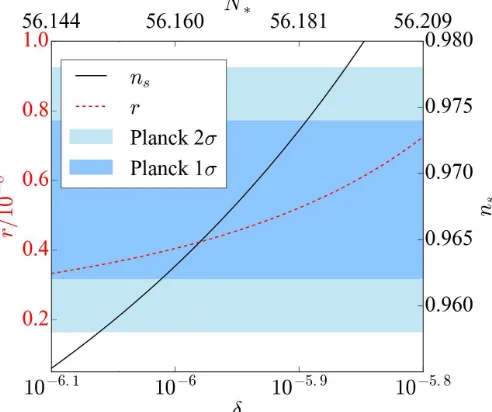
The spectral index and tensor-to-scalar ratio for this model are calculated for varying positiveδvalues and the parameter space satisfying the Planck results is presented in TableI, along with the values of N∗,Ntot and the run-ning of the spectral index. Using the Planck 2−σconstraint ofns= 0.968±0.010[1], provides limits onδ:
10−6.06≤δ≤10−5.86. (15) It is clear that, for the region where the spectral index and tensor-to-scalar ratio values match observations,δis within the constraint of Eq. (14) such thatN∗ < Ntot and we do not need to worry about initial conditions.
The model’s predictions for the inflationary observables are shown in TableIand Fig.1.
δ N∗ Ntot ns r/10−9 n0s/10
−6
10−5.80 56.21 120.99 0.987 7.24 -3.72
10−5.85 56.19 128.18 0.980 6.07 -3.11
10−5.90 56.18 135.79 0.973 5.21 -2.67
10−5.95 56.17 143.84 0.968 4.55 -2.33
10−6.00 56.16 152.38 0.963 4.04 -2.07
10−6.05 56.15 161.23 0.959 3.64 -1.86
[image:3.612.347.536.41.172.2]10−6.10 56.14 171.00 0.955 3.32 -1.70
TABLE I:δ values producingns within the Planck 2-σ
bounds.
NEGATIVEδ VALUES AND QUANTUM
TUNNELLING
When δ is negative, the potential develops a local min-imum and maxmin-imum in place of a flat plateau. When the inflaton field tunnels through the local maximum, it may be in a position to slow-roll on the other side of the peak, hope-fully for enough e-folds to generate nsandrin accordance
with observations. We calculated the number of slow-roll e-folds from the exit point of the quantum tunnelling and found that they are enough only whenδ≥ −10−8and in all cases N∗ = 56.08. Even though this is a similar e-folding
number to our results in the positive delta case, because the
FIG. 1: Values ofδfor whichns (solid black line) andr
(dashed red line) fall within the Planck bounds forns
depicted with the shaded horizontal bands (light: 2-σand darkened: 1-σ). The top axis also shows the correspondingN∗ values for eachδvalue. (CMB only
[image:3.612.320.566.424.630.2]delta value is constrained to be a lot smaller it only results inns= 0.928 which is unacceptable because the spectrum
is too red.
HIGHER-ORDER NON-RENORMALISABLE TERM
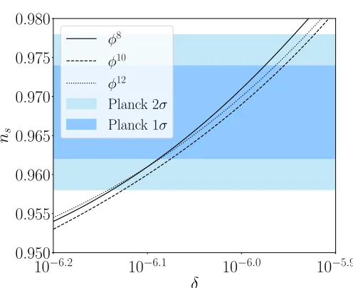
Let us now consider higher values of n; the order of the non-renormalisable operator in Eq. (6). It is straight-forward to check that our findings in the n= 1 case are largely unchanged. As shown in Tables III, IV and V, for n= 2,3,4, we find ns within the 2-σ Planck bounds
only when 10−6.2< δ <10−5.9. We also findn0
s∼ −10−6,
N∗≈56,Ntot>2N∗ andr∼10−(9−10). Our results show
r'0, with very small differences for varyingn, and changes innsfor varyingnare at the 10−3level. It should not be a
surprise that our results are robust and largely independent ofn, as is clearly shown in Fig. 2. By the time the cosmo-logical scales leave the horizon the field has rolled passed the inflection point and the scalar potential is dominated by the CW-term in Eq. (5),which isnindependent.
n 1 2 3 4
[image:4.612.323.559.28.649.2](φf/mP)2n 1.65 1.00 0.61 0.37
TABLE II: Values of (φf/mP)2n forn≥1.
The value of the field at the inflection pointφf reduces
somewhat for largern. Indeed, it is easy to show that the generalisation of Eq. (9) for arbitrarynis
φf =e 1 2n(1−
n
2)mP and αf≡ 2e
n
2−1
n(n+ 2). (16)
The above suggest that (φf/mP)2n=e1− n
2, which means
that (φf/mP)2n.0.1 for n≥4 (see Table II). This
im-plies that, becauseφ < φfwhen the cosmological scales exit
the horizon (N∗ < Ntot/2), we would expect high-order non-renormalisable terms to be suppressed when n >4. Thus, it is unlikely that the dominant, stabilising, non-renormalisable operator would correspond ton >4.
δ N∗ Ntot ns r/10−10 n0s/10
−6
10−5.9 56.04 123.60 0.984 8.51 −3.48
10−6.0 56.01 138.70 0.971 6.2 −2.54
10−6.1 55.99 155.64 0.961 4.88 −1.99
10−6.2 55.97 174.65 0.954 4.05 −1.65
TABLE III: Results forφ8
δ N∗ Ntot ns r/10−10 n0s/10
−6
10−5.9 55.95 126.21 0.981 3.1 −3.27
10−6.0 55.93 141.81 0.969 2.30 −2.42
10−6.1 55.91 159.39 0.960 1.82 −1.92
[image:4.612.349.535.43.125.2]10−6.2 55.90 179.23 0.953 1.52 −1.60
TABLE IV: Results forφ10
δ N∗ Ntot ns r/10−10 n0s/10
−6
10−5.9 55.91 125.30 0.982 1.72 −3.35
10−6.0 55.88 142.71 0.970 1.29 −2.51
10−6.1 55.86 158.58 0.961 1.03 −2.00
[image:4.612.103.236.316.345.2]10−6.2 55.85 172.96 0.954 0.87 −1.68
TABLE V: Results forφ12
10
−6.210
−6.110
−6.010
−5.9δ
0.950
0.955
0.960
0.965
0.970
0.975
0.980
n
sφ8
φ10
φ12 Planck 2σ Planck 1σ
FIG. 2: Values ofδfor whichnsfalls within the Planck
bounds depicted with the shaded horizontal bands (light: 2-σand darkened: 1-σ) for varying orders of the
[image:4.612.318.566.418.620.2] [image:4.612.79.262.565.646.2]INFLATIONARY SCALE AND FINE-TUNING
We determine the inflationary energy scale via the COBE constraint:
V1/4= 0.013r1/4mP. (17)
As shown in Table I and Tables III, IV and V, for δ∼10−6, we have r
∼10−(9−10). Thus, the above sug-gests thatV1/4
∼1014GeV. Now, from Eq. (8), we have5
V1/4
∼β1/4φ. Using the fact thatφ
∼φf ∼mP we obtain
β ∼ 10−16. Because β=y4/32π2, we find y
'4×10⁻⁴,
which is a very reasonable value for a Yukawa coupling and in agreement with the assumptiony1 (see Eq. (4) and footnote 2). Through Eq. (7), we then determine M = 2√π(2β)1/4m
P '1015GeV; near the grand
unifica-tion scale and sub-Planckian as expected.
Inflection-point inflation involves fine-tuning to attain the necessary inflationary plateau. In loop inflection-point inflation the tuning6 is δ∼10−6. This is exponen-tially better than the tuning corresponding to the horizon and flatness problems, resolution of which is one of the main motivations of inflation. For example, at the scale V1/4
∼1014GeV, the deviation from flatness needs to be
|Ω−1|.10−40. Note also, that δ
∼10−6 is much better than the level of tuning required in A-term/MSSM infla-tion [4].
It is important to note here that the assumption of slow-roll is not always justified in inflection-point inflation mod-els. This is because the potential near the inflection-point is so flat that the system may depart from slow-roll and temporarily engage into so-called ultra-slow-roll (USR) in-flation [13]7. This can have profound implications on the calculation of inflationary observables and may invalidate our findings (as well as those of most of the inflection-point literature). However, this danger can by averted if we assume that the inflaton lies initially near the inflec-tion point with small enough kinetic density. In Ref. [14] it is shown that, when the original kinetic density satisfies the boundρkin≤(V0mP)2/6V at the inflection point, then
slow-roll inflation begins immediately and all our findings are reliable. In our model V ∼β m4
P and it can be
eas-ily shown that V0(φf)∼βδ m3P. This means that, if the
inflaton starts near φf with kinetic density ρkin .βδ2m4P
then slow-roll inflation begins immediately and our findings are fine. Putting in the numbers, we findρ1kin/4.1011GeV,
5Strictly speaking, Eq. (8) considers n = 1. However, observ-able inflation occurs after the inflaton field crosses the inflection point φf, which means that the CW term dominates over the non-renormalisable term in Eq. (8). Thus, the order of the non-renormalisable term is not relevant here and V1/4 ∼ β1/4φfor n >1 too.
6This does not take into account the tuning required to satisfy Eq. (7). However such tuning is rather small since Eq. (7) is satisfied for quite natural values of the parameters.
7We would like to thank C. Germani for pointing this out.
0
20
40
60
80
N
−
1.0
−
0.5
0.0
0.5
1.0
&
η
φ/φ
fη
0.75
0.80
0.85
0.90
0.95
1.00
φ/φ
[image:5.612.319.567.43.218.2]f
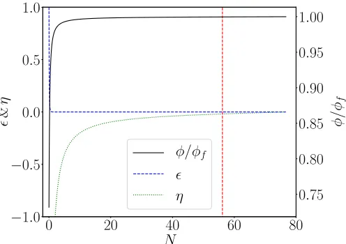
FIG. 3: The values of the inflaton field φ(solid black line) and the slow-roll parameters(dashed blue line) andη (dotted green line) with respect to the remaining e-folds
of inflationN are shown. The system progresses from right to left and inflation ends whenN = 0. The vertical
(dashed red) line denotesN∗, which corresponds to the
time when the cosmological scales exit the horizon during inflation. The inflaton is taken to roll from the inflection
point atφf with negligible initial kinetic density, such
that the slow-roll attractor is immediately assumed. As shown,is kept exponentially small during inflation. Inflation ends when= 1, with |η|becoming large in the
last e-fold of inflation, corresponding to a substantial variation of, that ends inflation.
i.e. a factor of 103 smaller than the energy scale of infla-tion. In Fig. 3 we track the evolution of the inflaton field and slow-roll parameters during inflation to demonstrate the avoidance of USR for negligible initial kinetic energy densities at the inflection point. Note that the issue of the initial conditions of inflation is academic because of the no-hair theorem, which demonstrates that memory of the initial conditions is lost once the inflationary attractor is attained.
REHEATING
A theory withV ∼βφ4, whenV00> H2leads to coherent oscillations in a quartic potential, whose density scales as radiation ρ∝a−4 [15]. This means that the amplitude of the oscillations decreases as φ∝1/a. These oscillations correspond to particles of massm∼√β φ∝1/a, which is redshifted similarly to radiation particles [16].
fermions produced by the inflaton decay are coupled to SM particles such that, once formed, they promptly decay into the radiation bath of the hot big bang.
Therefore, reheating occurs when areh
aend ∼
Hend Γend ∼
1
√
β 8π y2
Hend
φend
, (18)
where ‘reh’ denotes the moment of reheating. Using that the amplitude of the oscillations decreases asφ∝1/a, the above gives
φreh∼
y2√β 8π
φ2 end
Hend
. (19)
For the density of the oscillating condensate we have
ρreh=ρend
aend
areh
4
∼9β
y2 8π
4
m4P, (20)
where we usedρend∼Vend∼βφ4endandH 2
end=ρend/3m2P.
For the radiation bath we have ρreh= (π2/30)g∗Treh4 , whereg∗is the effective relativistic degrees of freedom and
Treh is the reheating temperature. Using this, the above equation suggests
Treh∼
270 π2g
∗
1/4y2β1/4
8π mP ∼0.03y
2β1/4m
P, (21)
where we considered thatg∗=O(100).8 Putting the
num-bers we obtained: y'4×10⁻⁴ and β
∼10−16, we get
Treh∼106GeV, which is comfortably higher than the tem-perature at BBN (∼1 MeV) but low enough to avoid the generation of dangerous relics (e.g. gravitinos).
Now suppose that there is also a quadratic term in the scalar potential such that the inflaton has a bare massm0 and V ∼m20φ2+βφ4. In order not to influence inflation, the quadratic term must remain negligible during inflation. This meansm2
0< βφ2. Usingβ∼10−16andφ∼φf ∼mP,
we find the boundm0<1010GeV.
In order not to influence reheating the bound on m0 is much more stringent, because we need the quadratic term in the potential to remain subdominant until the decay of the inflaton condensate, that is we need m2
0< βφ2reh. In view of Eq. (19), we get
m0<
p
3β y
2
8πmP, (22)
where we also considered that H2
end'Vend/3m2P and
Vend∼βφ4end. Putting the numbers in, we obtain
m0<300 GeV or so. This is a bit tight but it also means that ifm0∼1 TeV, the influence on the value ofN∗ would
be of the order ∆N∗' 16ln(m20−βφ2reh)<1, which would have minimal impact on our results, while a TeV-scale scalar particle might be observable in the LHC in the near future.
8This is Eq. (108) of Ref. [16].
CONCLUSIONS
To conclude, we have studied a simple but elegant in-flation model, where the inin-flationary plateau is gener-ated through the running of the self-coupling of a mass-less scalar field, stabilised by a non-renormalisable oper-ator. We have found that the model accounts for ob-servations with mild tuning of the order ∼ 10−6 and a natural value of the Yukawa coupling y'4×10⁻⁴. In particular, the model can result in the spectral index of the scalar curvature perturbation within the 1-σbound of the latest CMB observations, while producing negligible tensors (r∼10−(9−10)). The inflationary energy scale is
V ∼1014GeV; much higher that A-term/MSSM inflation (hence, the tuning is less). We also studied perturbative reheating in our model and obtained a reasonable reheat-ing temperature Treh∼106GeV. Non-perturbative effects might enhance the efficiency of reheating. Our setup is minimal and does not require exotic physics apart from the non-renormalisable term.
Acknowledgements KD is supported (in part) by the Lancaster-Manchester-Sheffield Consortium for Fundamen-tal Physics under STFC grant: ST/L000520/1. CO is ported by the FST of Lancaster University. AR is sup-ported by the Estonian Research Council grants IUT23-6, PUT1026 and by the ERDF Centre of Excellence project TK133.
[1] P. A. R. Ade et al. [BICEP2 and Keck Array Collabora-tions], Phys. Rev. Lett.116(2016) 031302.
[2] K. Dimopoulos and C. Owen, Phys. Rev. D94(2016) no.6, 063518
[3] R. Allahverdi, A. Kusenko and A. Mazumdar, JCAP0707
(2007) 018.
[4] J. C. Bueno Sanchez, K. Dimopoulos and D. H. Lyth, JCAP
0701(2007) 015.
[5] R. Allahverdi, K. Enqvist, J. Garcia-Bellido and A. Mazum-dar, Phys. Rev. Lett.97(2006) 191304; D. H. Lyth, JCAP
0704 (2007) 006; R. Allahverdi, K. Enqvist, J. Garcia-Bellido, A. Jokinen and A. Mazumdar, JCAP0706(2007) 019; K. Enqvist, L. Mether and S. Nurmi, JCAP 0711
(2007) 014; R. Allahverdi, A. Ferrantelli, J. Garcia-Bellido and A. Mazumdar, Phys. Rev. D83(2011) 123507. [6] N. Itzhaki and E. D. Kovetz, JHEP 0710 (2007) 054;
M. Badziak and M. Olechowski, JCAP 0902(2009) 010; K. Enqvist, A. Mazumdar and P. Stephens, JCAP 1006
(2010) 020; S. Hotchkiss, A. Mazumdar and S. Nadathur, JCAP1106(2011) 002; N. Okada and D. Raut, Phys. Rev. D95(2017) no.3, 035035.
[7] Y. Hamada, H. Kawai, K. Y. Oda and S. C. Park, Phys. Rev. Lett. 112 (2014) no.24, 241301; F. Bezrukov and M. Shaposhnikov, Phys. Lett. B734(2014) 249; G. Balles-teros and C. Tamarit, JHEP1602(2016) 153; N. Okada, S. Okada and D. Raut, Phys. Rev. D 95 (2017) no.5, 055030.
[9] R. H. Brandenberger, A. Nayeri, S. P. Patil and C. Vafa, Int. J. Mod. Phys. A22(2007) 3621.
[10] K. Kannike, G. H¨utsi, L. Pizza, A. Racioppi, M. Raidal, A. Salvio and A. Strumia, JHEP1505(2015) 065; M. Ri-naldi, L. Vanzo, S. Zerbini and G. Venturi, Phys. Rev. D 93 (2016) 024040; A. Farzinnia and S. Kouwn, Phys. Rev. D93 (2016) no.6, 063528; L. Marzola, A. Racioppi, M. Raidal, F. R. Urban and H. Veerm¨ae, JHEP1603(2016) 190; L. Marzola and A. Racioppi, JCAP1610(2016) no.10, 010; M. Artymowski and A. Racioppi, JCAP1704(2017) no.04, 007.
[11] S. R. Coleman and E. J. Weinberg, Phys. Rev. D7(1973) 1888.
[12] M. S. Turner, Phys. Rev. D28(1983) 1243.
[13] W. H. Kinney, Phys. Rev. D 72 (2005) 023515; J. Mar-tin, H. Motohashi and T. Suyama, Phys. Rev. D87(2013) no.2, 023514; M. H. Namjoo, H. Firouzjahi and M. Sasaki, Europhys. Lett.101(2013) 39001; A. E. Romano, S. Mooij and M. Sasaki, Phys. Lett. B761(2016) 119; C. Germani and T. Prokopec, arXiv:1706.04226 [astro-ph.CO].
[14] K. Dimopoulos, Phys. Lett. B 775(2017) 262 [15] M. S. Turner, Phys. Rev. D28(1983) 1243.