University of Warwick institutional repository: http://go.warwick.ac.uk/wrap
A Thesis Submitted for the Degree of PhD at the University of Warwick
http://go.warwick.ac.uk/wrap/57035
This thesis is made available online and is protected by original copyright. Please scroll down to view the document itself.
Essays in Applied Public Economics Using
Computable General Equilibrium Models
by
Erez Yerushalmi
A thesis submitted in partial fulfilment of the requirements
for the degree of
Doctor of Philosophy in Economics
Department of Economics
University of Warwick
Contents
List of figures vi
List of tables viii
Acknowledgements x
Declaration xii
Abstract xiii
Abbreviations xiv
1 Introduction 1
Water allocation (Part I) . . . 3
Malaria prevention (Part II) . . . 6
References . . . 9
Part I
Water allocation
11
2 Which is preferable for Israel, a market or an administrative water
allocation mechanism? 11
2.1 Introduction . . . 11
2.2.1 A simplified trade model with water inputs . . . 16
2.2.2 Secondary water market . . . 19
2.3 The applied general equilibrium model and the data . . . 21
2.3.1 Production . . . 22
2.3.2 Household . . . 24
2.3.3 General assumptions in the model . . . 24
2.3.4 Data and marginal value of water . . . 25
2.4 Measuring the efficiency of an administrative water allocation . . . . 27
2.4.1 Results for 2006 . . . 28
2.4.2 Sensitivity analysis . . . 31
2.4.3 Comparing results for 1995 through 2006 . . . 33
2.4.4 Policy implications . . . 36
2.5 Inferring the value of agricultural amenities . . . 36
2.5.1 Policy implication and results . . . 41
2.6 Conclusions . . . 43
3 Water policy in Israel and the water model 45 3.1 The history of water management in Israel . . . 45
3.2 The recurrent water crisis in Israel . . . 47
3.3 A water market as an alternative to the administrative mechanism . . 50
3.4 A full description of the applied water model . . . 54
3.4.1 Production structure . . . 55
3.4.2 Household utility structure . . . 60
3.4.3 Balance of payments and market clearing conditions . . . 62
3.4.4 Secondary potable water market . . . 63
3.4.5 Agricultural amenity . . . 66
3.5 Calibrating substitution elasticities in production . . . 68
3.6 Calibrating substitution elasticity in household utility . . . 72
3.7 Data collection and building the SAM . . . 74
3.7.1 Social accounting matrix . . . 74
3.7.2 Water consumption by user and water prices . . . 75
3.8 Conclusion . . . 76
References for part I: water allocation . . . 77
Part II
Malaria prevention
87
4 Estimating the macro-economic impact of malaria: a case study of Ghana (with P. Hunt and S. Hoorens) 87 4.1 Introduction . . . 874.2 Malaria and its social and economic consequences . . . 90
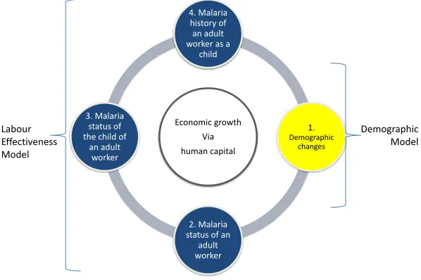
4.2.1 Demographic changes and mortality (first component) . . . 92
4.2.2 Labour effectiveness (second component) . . . 93
4.3 Ghana case study . . . 97
4.4 A dynamic general equilibrium model for Ghana . . . 101
4.4.1 A description of the model . . . 103
4.4.2 Recursive dynamics . . . 105
4.4.3 Integrating health into the DCGE model . . . 107
4.5 Population projection model . . . 108
4.5.1 Baseline projections using a cohort-component method . . . . 109
4.5.2 Malaria prevention scenarios for children under 5 years . . . . 112
4.6 Labour efficiency model . . . 114
4.7 Limitations and discussion . . . 116
4.8 Results . . . 118
4.8.1 The benefit of treatment per individual covered . . . 123
4.8.3 Sensitivity analysis . . . 125
4.9 Conclusion . . . 126
5 The malaria model 128 5.1 The model . . . 128
5.2 Production . . . 130
5.2.1 Domestic production . . . 130
5.2.2 Transformation between domestic use and exports . . . 133
5.3 The Armington assumption . . . 135
5.4 Government behavior . . . 137
5.5 Household behaviour . . . 140
5.5.1 Recalibrating the SAM with subsistence level . . . 143
5.6 Market clearing conditions . . . 144
5.7 Rest of the world (ROW), international trade, and capital flow . . . . 144
5.7.1 International trade . . . 146
5.7.2 Capital flow and net foreign assets . . . 146
5.7.3 Trade balance and the current account . . . 148
5.8 Investment and savings in the capital market . . . 148
5.9 Recursive dynamics . . . 149
5.9.1 Capital accumulation . . . 151
5.9.2 Updating labour recursively from the health models . . . 154
5.9.3 Updating recursively other variables . . . 156
5.10 The values used for the model parameters . . . 158
5.10.1 Income elasticities of demand . . . 158
5.10.2 Other deep parameter . . . 159
5.11 Conclusion . . . 160
List of Figures
2.1 Water quotas with two agents . . . 16
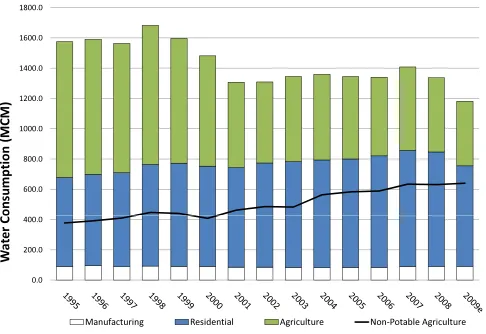
2.2 Potable water consumption by main users (MCM) . . . 35
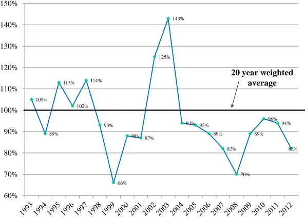
3.1 National weighted rainfall as percent of the 20 year average . . . 47
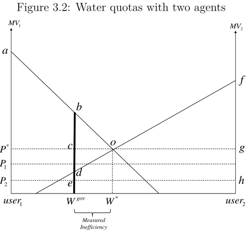
3.2 Water quotas with two agents . . . 52
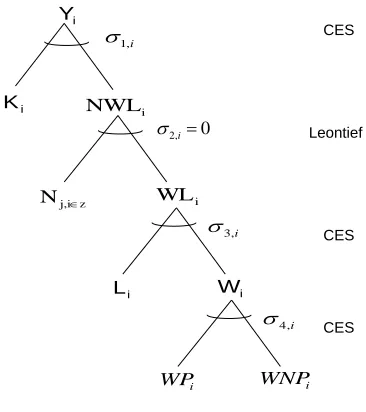
3.3 The production function . . . 56
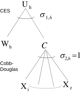
3.4 Household utility . . . 61
4.1 A typology of the effects that malaria has on economic growth . . . . 92
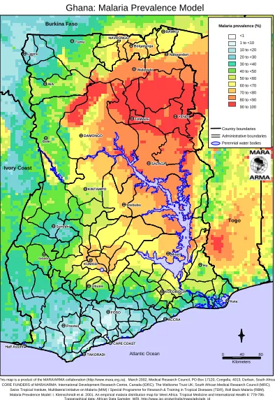
4.2 Malaria prevalence in Ghana . . . 98
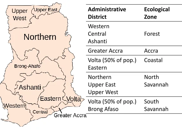
4.3 Mapping administrative districts to ecological zones . . . 99
4.4 Number of under five year covered (millions) . . . 103
4.5 A diagrammatic representation of the DCGE model . . . 107
4.6 Proportion of death by cause by zone . . . 114
4.7 Income per capita relative to baseline (% change) . . . 120
4.8 Richest 20/poorest 20 income relative to baseline (% change) . . . 120
4.9 Annual average income per capita relative to baseline (% change) . . 122
4.10 Income per capita relative to baseline, by zone and urbanity (average over 30 years) . . . 122
4.11 Income-benefit per covered individual, 2007 US$ . . . 123
List of Tables
2.1 Key water figures in Israel (2006) . . . 22
2.2 Output-supply-price and demand-price elasticities . . . 23
2.3 Water trade channels: relative MVW for 2006 . . . 27
2.4 Model results (2006, % change) . . . 29
2.5 Other key results (2006, % change) . . . 30
2.6 Values used for sensitivity analysis, 2006 . . . 31
2.7 Secondary water markets for 1995-2006 . . . 33
2.8 Potable water expenditure as % of total cost (net of tax) . . . 34
2.9 Agriculture amenity value (2006) . . . 39
3.1 Calibrating the substitution elasticities, SAM 2006 . . . 69
3.2 Water price by user (yearly average) . . . 76
4.1 Adult worker lost production days and productivity due to malaria illness 94 4.2 Days lost due to caring for children with malaria . . . 95
4.3 Impact of malaria as a child for labour productivity later in life . . . 96
4.4 Key statistics on malaria in Ghana, 2009 . . . 97
4.5 Malaria prevalence (%) by region and age groups of Ghana, 2002 . . . 100
4.6 Coverage of the preventative malaria intervention in the baseline and three alternative scenarios . . . 102
4.8 Key assumptions and parameter values of the labour effectiveness index 116
4.9 Additional value compared to baseline, year 1-30 . . . 118
4.10 Regional benefit per treated individual (2007 US$, average of year 1-30)124
4.11 Sensitivity analysis . . . 126
Acknowledgements
I would like to express my sincere gratitude to my supervisors, Carlo Perroni and Lei
Zhang, for their help and guidance throughout this research. I also greatly appreciate
the financial support that I have received from the Vice-Chancellor of the University
of Warwick, and from the Department of Economics.
For the first part of the thesis, Water Allocation, I would like to thank the
Is-raeli Water Authority for data. My appreciation is also extended to Peter Backus,
Jonathan Cave, Alessandro Iaria, Clara Rübner Jørgensen, Alex Klein, Michael
Wa-terson, and Paul Youdell for stimulating discussions and much appreciated help, and
to Jesper Jensen on related research. Many thanks to the conference participants
of Emerging Issues in Agricultural Economics, Hebrew University in Rehovot, June 2011, for their comments on the preliminary results and conclusion; particularly Eli
Feinerman, Israel Finkelshtain, Barry K. Goodwin, David A. Hennessy, Iddo Kahn,
Ayal Kimhi, Yoav Kislev, and Yakov Tsur.
For the second part of the thesis,Malaria Prevention, I would like to acknowledge
the financial support of GlaxoSmithKline (GSK) Vaccines. Many thanks to my
co-authors, Priscillia Hunt and Stijn Hoorens, for good team work and for introducing
me to Health Economics. Our cooperation has been a joint learning process. We
are grateful to James Thurlow and Xinshen Diao from the International Food Policy
Research Institute (IFPRI) and other authors for providing us the Ghana Social
data available, our research would not have been possible. We also thank Patricia
Akweongo, Jonathan Cave, Jeffrey Round and Simo Goshev for good discussions,
advice, and much appreciated suggestions, and Shelly Culbertson, Jirka Taylor, and
Benoit Guerin for research and editorial support. My special thanks goes to Richard
Smith and Christophe Sauboin for their comments on earlier drafts of Chapter 4.
Finally, I would like to thank my wife, Clara, for all her help. She has been on
this journey with me, while finalising her own PhD, and has given me two beautiful
Declaration
I declare that the thesis is my own work and has not been submitted for a degree at
another university.
Erez Yerushalmi
Abstract
This thesis analyses two issues in public economics: (1) water allocation in Israel; and (2) malaria prevention in Ghana. In both cases a computable general equilibrium modelling approach has been applied for policy analysis.
Part I: In Israel, parliamentary investigative committees and water researchers have concluded that for decades, the administrative water allocation mechanism has mismanaged water allocation. Over subsidising of the agricultural sector, and un-derfunding of desalination plants, had led to a severe hydrological deficit. Critics argue that a water market allocation could solve these issues. However, the adminis-trative allocation is crucial because it protects social value, which is not represented in a market mechanism. Part I of the thesis compares these two alternative alloc-ation mechanisms using a general equilibrium model, for the case of Israel. The model concludes that from 1995 to 2006, the upper-bound water misallocation in Israel was relatively small, on the average of 5.5% of the potable water supply. The lower-bound value of agricultural amenities is imputed at approximately 2.3 times agricultural economic output. At the margin, introducing a water market in Israel is
not recommended, i.e., net-social welfare would fall.
Abbreviations
<5 - Under five years old
CBS - Central Bureau of Statistics in Israel
CES - Constant Elasticity of Substitution
CET - Constant Elasticity of Transformation
CGE - Computable General Equilibrium
DCGE - Dynamic Computable General Equilibrium
GDHS - Ghana Demographic and Health Surveys
GHS - Ghana Health Service
GSK - GlaxoSmithKline
GSS - Ghana Statistical Services
IBT - Increasing Block Tariff
IFPRI - International Food Policy Research Institute
MCM - Million Cubic Meters
MVW - Marginal Value of Water
ROW - Rest of the World
SAM - Social Accounting Matrix
SOE - Small Open Economy
TFR - Total Fertility Rate
Chapter 1
Introduction
This PhD thesis examines two separate themes within applied public economics. Part
I discusses water allocation and compares the benefits of an administrative water
allocation mechanism in Israel, to a market mechanism. Part II deals with the issue
of malaria prevention and assesses the economic impact of malaria prevention on the economy in Ghana. In both, computable general equilibrium (CGE) modelling is
used to analyse and discuss the implications of alternative policies.
Policy analysis is a process by which researchers analyse the various components
relating to a specific issue, define appropriate goals, propose alternative policies, and
examine their interactions and results. Models are used when it is infeasible to
exper-iment on real economies, for example because of size limitations, the issue at hand,
or the time frame. There are, however, several modelling techniques to choose from,
and as Box and Draper (1987) famously wrote: “...all models are wrong, but some
are useful.” This thesis employs applied CGE modelling, which is a useful simulation laboratory for quantitatively assessing the effects of external shocks and/or policies
on the economy.
As discussed by Dervis et al. (1982); Shoven and Whalley (1992); Mas-Colell et al.
view the many markets of goods and inputs as an interrelated system, whereby values
at equilibrium for all variables are simultaneously determined. Consumers maximize
utility subject to their budget constraint, forming the demand-side of the model,
while producers maximize profits, forming the production-side of the economy. In
equilibrium, prices adjust so that equilibrium must hold, and demand equals supply.
In cases with constant returns to scale (CRS), zero profit conditions are satisfied for
each industry.
Furthermore, general equilibrium is based on the Arrow-Debreu theorem that
provides a proof of a given equilibria (Arrow and Debreu, 1954). This fixed point
theorem is essential for policy issues because before attempting to compute the
equi-librium of the model, and compare it to counter-factual scenarios, it is necessary to
first believe that equilibrium exists.
Applied CGE modelling is now a standard tool of empirical analysis. It is
predom-inantly used for analysing policy issues, such as income distribution, trade policy,
en-vironment, structural adjustments to external shocks, growth and structural changes,
government tax (subsidy) policy, etc.
The two themes discussed in this thesis focus on environmental issues and external
shocks to labour resources. To analyse such themes, other modelling approaches, such
as partial equilibrium, may in principle be sufficient. However, partial equilibrium
only examines the direct effect of a limited component while keeping all other effects
fixed. If we believe that the endogenous inter-linkages between the various markets is
an important element in the analysis, and that the indirect effects are sizeable, then
general equilibrium methods are needed. Furthermore, alternative policy scenarios
cannot be similarly assessed using partial equilibrium techniques.
CGE models most often simulate comparative static results, an approach used in
the water allocation model in Part I of this thesis. In the last decade, it has, however,
looking approach, or arecursive (myopic) approach. The latter is used in the malaria prevention model in Part II of the thesis.
Finally, a number of additional features can be added to CGE models,e.g., varying
“closure rule” assumptions, imperfect competition, imbalances, and various structural
and institutional rigidities. These are all approaches that I have worked with during
the PhD studies and in the development of my research. For example, the water
allocation model uses a re-calibration approach to impute the value of the agricultural
amenity, while the malaria prevention model started-off as a forward-looking “toy”
model, and due to computational constraints, was later converted into a recursive
model.
Water allocation (Part I)
Part I of the thesis, discusses water allocation and uses Israel as a case study. It
is motivated both by my personal experiences as a child in Israel, and my academic
interest in the allocation of limited resources. In the mid ’70s through the ’90s, I grew
up in a small village approximately 20 kilometres south of Tel-Aviv. As a hobby, my
parents have cultivated more than 70 different types of fruit trees, a vegetable patch,
and small vineyard. Hundreds of acres of citrus fruits were grown around my house,
and I have many fond memories of the agricultural landscape surrounding me.
Today, my “jungle” playground has, however, nearly dried-up, and is gradually
being replaced by lucrative housing projects. My childhood village is steadily being
absorbed by the nearest city, claiming it as one of its many neighbourhoods. With
urbanization has come modern infrastructure, such as street lamps, a modern sewer
system, and the city water supply. However, until 2001, water supply came from the
village’s own water well, and water prices were under agricultural tariffs, which were
substantially lower than city water tariffs. (See Table 3.2 in Chapter 3.)
Mediterranean countries, is a limited resource. How to allocate it efficiently, how to
decide who owns the resource, and how to protect it, are all very important questions.1
In 1959, a Water Law was enacted to control and protect Israel’s water resources, and
an administrative body called theWater Authority was empowered to allocate water.
The main tool of the Water Authority is to classify water users according to different
characteristics, e.g., households, industrial, or agricultural users, and then assign to
them different water quotas, water tariffs, and increasing block tariff structures. In
order to enforce the administrative allocation, water resale is prohibited, and this
further disconnects market forces from the pricing and allocation of water.
Similar to many households that were living in rural areas, but were not agrarian,
my parents and our neighbours benefited from household water consumption at
ag-ricultural prices. However, the largest of such irregularities probably originated from
the communally organized kibbutzim and moshavim that used a sizeable portion of
agricultural water for non-farming activities and/or businesses, e.g., a recreational
swimming pool, or a “black” water market. With the gradual urbanization of the
country, these irregularities were reduced, and tighter regulatory control of the water
resource was enabled. However, it could be argued that this came at the cost of the
rural environment.
The depletion of the water reserves in Israel has seriously damaged water quality.
Excess pumping from water reserves over many years has caused a hydrological deficit
of the most severe proportions. Every few years, when annual rainfall is very low,
the Israeli Government announces a “Water Crisis.” Critics (e.g., Plaut, 2000) argue
that this illustrates why an administrative mechanism cannot accurately account for
the true environmental value of water, and why it often misallocates water compared
to a market mechanism. An administrative mechanism is politicized, subjective, and
slow to respond to weather conditions and population needs. Furthermore, the
over-subsidization of agricultural water has driven farmers to increasingly grow low-revenue
water-intensive crops. In some sense, it could be argued that a portion of the water
resources in Israel are “exported”, as embodied by farm exports.
Using a traditional CGE approach, to evaluate these arguments, would naturally
favour a water market because it allows water inputs to flow to those users valuing
them the most. In this thesis, however, I recognize that an administrative mechanism
also promotes social goals that are not valued economically, such as green areas, food
security, rural environment, and population dispersion. The main contribution in this
part of the thesis is to compare two alternative allocation mechanisms in a context
of erroneous policy choices. A type I error would be to introduce a water market,
but then lose social welfare in the form of reduced agricultural amenities. A type II
error would benot to introduce a water market, and therefore to inefficiently allocate water by an administrative mechanism.
Weighing the outcomes of these two errors, I find that at the margin, introducing
a water market in Israel is not recommended, i.e., net-social welfare would fall. In
addition, infra-marginal social losses could be even larger, if other forms of amenities
were to be included,e.g., the loss to historical heritage, and especially the irreversible
destruction of nature.
Part I of the thesis thus relates to two areas of research. It has relevance for natural
resource management that aims to improve the efficient use of a scarce resource, and
it has implications for political and social policy. Chapter 2 of the thesis is aimed
as a future journal paper. It presents the issue, summarizes the main results, and
discusses their policy implications. Chapter 3 of the thesis contextualises water policy
Malaria prevention (Part II)
Part II of the thesis focuses on malaria prevention in Ghana. This work is partially
funded by GlaxoSmithKline (GSK), and is a result of a joint research effort with
RAND Europe. It is motivated in spirit by the health targets of the Millennium
Development Goals, mainly Goal 4, which is to reduce child mortality, and Goal
6, which is to combat HIV/AIDS, malaria and other diseases (WHO, 2005). More
specifically, the aim is to assess the economic and distributional impact of malaria
prevention in an endemic country.
A variety of agencies, who work either cooperatively or individually, are involved in
combating malaria. These include governments of malaria-endemic countries, donor
countries, international bodies, international firms, and private individuals.2 GSK
is one of the largest international pharmaceutical firms, and is directly involved in
developing anti-malarial drugs and vaccines.3
In 2010, the economics department of GSK Vaccines decided to fund an academic
research project on malaria, with the intention that it will be published in a peer
reviewed journal. RAND Europe was contracted to carry out the research, and I was
invited to join the team. Consequently, I took a lead role in the research: I designed
and programmed the dynamic computable general equilibrium (DCGE) model (from
scratch), and we shared equal burden on other aspects of the project. Due to my
level of contribution, we agreed that I am the first and corresponding author on the
future journal paper.
So far, research on the link between malaria and economic growth has used
econo-metric methods. These give, however, results which are too broad and not particularly
useful for policy analysis. Furthermore, critics argue that they over-state the benefits
2International bodies include the World Bank, WHO, and the GAVI Alliance. A well-known individual donor is the Bill and Melinda Gates Foundation.
of malaria reduction because they do no include general equilibrium effects, especially
those of diminishing returns to effective units of labour (e.g., Acemoglu and Johnson,
2007).
Our research fills this gap, and provides a more detailed estimate of the impact of
malaria at various levels,e.g., household, regional, and/or age level. This is important
for policy makers who must operate within a limited budget, and require information
to design malaria intervention policies. On the same note, pharmaceutical firms, who
are negotiating with government and donors on the provision of drugs and vaccines,
have an interest in understanding market demands and communicate opinions. This
approach is useful for cost-benefit methods, which are not commonly used in health
policy. Finally, it has the potential to be similarly used to assess other diseases,e.g.,
TB, HIV/AIDS, and obesity.
In the research, we simulate the impact of reducing malaria morbidity and
mor-tality on the Ghanaian economy utilising a micro-based approach. A multi-sector,
multi-agent, recursive DCGE model is developed and linked to (1) regional
demo-graphics with cohort-component projections for fertility, mortality, migration, and
urbanization; and (2) labour effectiveness indices for production and productivity of
parents with sick children, or adults affected by malaria during childhood. The model
is calibrated to Ghana, with households disaggregated by five epidemiological malaria
regions, urban-rural divide, and five income level quintiles. Hypothetical intervention
scenarios simulate reducing malaria prevalence by 50% for children under-five years
and with varying degrees of coverage.
The project is still on-going, and we are currently working on additional
counter-factual scenarios that represent other possible health provision strategies. The final
results submitted to a journal, may be slightly different from those presented here. In
general, however, we find that malaria prevention clearly adds to economic growth and
under-five year old population is treated. In this case study of Ghana, the benefits from an
intervention, per child covered, vary across regions, and generally contributes more
to the high prevalence regions.
Chapter 4 of the thesis is a joint effort with Pricillia Hunt and Stijn Hoorens, and
is aimed as a future journal paper. It describes the methodology by which we link
malaria and economic growth, discusses policy issues, and summarizes the results of
three hypothetical health intervention policies. Chapter 5 of the thesis is a detailed
References
Acemoglu, D. and S. Johnson: 2007, ‘Disease and Development: The Effect of Life
Expectancy on Economic Growth’. Journal of Political Economy115(6), 925–985.
Agnandji, S. T., B. Lell, S. S. Soulanoudjingar, J. F. Fernandes, and et. al.: 2011,
‘First Results of Phase 3 Trial of RTS,S/AS01 Malaria Vaccine in African Children’.
New England Journal of Medicine365(20), 1863–1875. (See full list of author names in journal appendix).
Arrow, K. J. and G. Debreu: 1954, ‘Existence of an Equilibrium for a Competitive
Economy’. Econometrica 22(3), 265–290.
Box, G. E. P. and N. R. Draper: 1987, Empirical Model-Building and Response
Sur-faces. Wiley, 1st edition.
Dervis, K., J. de Melo, and S. Robinson: 1982, General Equilibrium Models for
De-velopment Policy. Cambridge University Press.
Lofgren, H., R. L. Harris, and S. Robinson: 2002, A Standard Computable General
Equilibrium (CGE) Model in Gams. International Food Policy Research Institute (IFPRI).
Mas-Colell, A., M. D. Whinston, and J. R. Green: 1995, Microeconomic Theory.
Oxford University Press, USA.
Plaut, S.: 2000, ‘Water Policy in Israel’. Policy Studies 47, Institute for Advanced
Strategic and Political Studies, Division for Economic Policy Research.
Shoven, J. B. and J. Whalley: 1992, Applying General Equilibrium. Cambridge
Uni-versity Press.
WHO: 2005, ‘Health and the Millennium Development Goals’. Technical report, World
Chapter 2
Which is preferable for Israel, a
market or an administrative water
allocation mechanism?
2.1
Introduction
Most arid and semi-arid regions use an administrative water allocation mechanism,
whereby the state monopolizes the water resource, and erects a regulatory body to
administer it. The main tools used are quotas, price discrimination, and increasing
block tariffs that are set and upheld by prohibiting the resale of water.1
Critics of this mechanism argue that allocation is subjective, politicized, and leads
to inefficiencies (Dinar et al., 1997; Holden and Thobani, 1996). Much of the criticism
centres on the agricultural sectors that have access to subsidized water. Farmers
appear to have historical, senior rights, and are shielded by a strong lobby. Therefore,
even when inefficiencies are detected, the political system finds it difficult to change
antiquated allotments. The result is inefficient use of water, whereby farmers grow
low-value and surplus crops, while non-agricultural water users struggle to develop
expensive new supplies (Colby, 1990; Plaut, 2000). In addition, a ’black’ water market
may form, which further indicates that water is misallocated (Lichtman, 2009).2
These arguments are partly justified, but as discussed by Just et al. (1997), the
goal behind an administrative allocation is to promote social objectives, such as
wa-ter and food security, or equitable consumption across income groups or climate
specific regions. Administrative mechanisms are also used to correct market-failures
in situations of public goods, where an amenity provides non-marketed services,e.g.,
agricultural landscape, tourism, and historical heritage. The multi-functionality of
agricultural activities may produce benefits over and above the market value of
agri-cultural production (Brunstad et al., 1999, 2005).
This chapter explores both positive and negative impacts of an administrative
water allocation using Israel as a case study. The following questions are addressed:
(1) Can the level of administrative misallocation be measured? (2) Who are the main
inefficient water users, and how can allocation be improved? (3) What value do the
amenities need to have in order to rationalize the current administrative allocation
as efficient? (4) Which is preferable, a market or an administrative mechanism?
To answer these questions, an applied general equilibrium model is developed and
calibrated to Israel from 1995 to 2006. In the initial case, a regulator decides on a
framework in which price discrimination, quotas, and increasing block tariffs are set,
and water trade is prohibited. Water users decide on the amount of water to buy
within this framework.
Subsequently, in the counter-factual experiments, water trade is enabled within
a secondary water market and prices adjust until markets clear. In the extension, the model accounts for the non-economic value of amenities, whereby the agricultural
sectors internalize the benefit of producing amenities demanded by the households.
If we consider the market allocation to be primarily efficient, the quantity of
water traded would indicate the level of administrative misallocation. For example,
a large secondary water market would indicate that the administrative mechanism is
inefficient, and that a market mechanism would put water to better use. If however
the social value provided by the administrative mechanism is also included, it is then
possible that the benefits from a water market could be smaller than the loss incurred
to social value, i.e., a net-social welfare loss.
Thus, two alternative allocation mechanisms can be compared in a context of
er-roneous policy choices. Atype I error would be to replace the current administrative
mechanism with a market mechanism, given that the current administrative
mech-anism is true (the null hypothesis H0). In this case, the loss to social welfare, in
the form of agricultural amenities, is greater than the gain in efficiency from a water
market. A type II error would be not to replace the administrative mechanism with
a market mechanism, given that the market mechanism is the correct policy. In this
case, the efficiency lost from not introducing a water market is larger than the social
value preserved in the form of agricultural amenities.
At the parametrization stage of the model, the approach is to calibrate the model
with (plausible) conservative parameters that would favour a market mechanism. On
the one hand, the calibration would lead to the largest plausible administrative water
misallocation, so that the potential size of a secondary water market is therefore a
conservative upper bounds. This raises the type II error. On the other hand, the
value of the agricultural amenity is aimed at being an underestimate lower bounds,
which lowers the type I error.
Nevertheless, the results find that the potential size of a secondary water market
(i.e., the administrative misallocation) is rather small, and when the model is
exten-ded to impute agricultural amenities, the amenity value is large. In other words, it
The potential social loss from introducing a market mechanism might be significantly
higher than the added benefits of efficient water use.
Furthermore, in the current analysis, only agricultural amenities are imputed.
Therefore, had additional amenities been considered (e.g., those stemming from
tour-ism, historical heritage, irreversible destruction to nature) the infra-marginal losses
from introducing a water market could be higher still.
The chapter makes the following contributions. First, it adds a new perspective
to the discussion of water allocation efficiency in Israel. Contrary to most literature
on Israel, the paper supports the continued use of an administrative water allocation
mechanism. Second, it suggests a simple method, which can be used to evaluate and
improve water allocation decisions also in other countries. Finally, the paper imputes
the value of agricultural amenities in Israel, adding to the discussion by Fleischer and
Tsur (2009) and Kan et al. (2009) on the economic value of agricultural amenities.
Thus, the paper relates to two areas of research. It has relevance for natural resource
management that aims to improve the efficient use of a scarce resource, and it has
implications for political and social policy.
The chapter is structured as follows: Section 2.2 discusses how inefficient water
allocation arises from an administrative mechanism and introduces a simplified
the-oretical model to estimate it. Section 2.3 expands to a more realistic multi-sector
applied general equilibrium model for the Israeli economy. Section 2.4 discusses the
empirical results. Section 2.5 extends the model to impute the value of the
agricul-tural amenities and discusses the policy implications of the results. Finally, Section
2.2
The water model
Applied general equilibrium models have been developed to analyse different issues
within water management (see Dixon, 1990; Berck et al., 1991; Seung et al., 2000; Diao
et al., 2008). Diao and Roe (2003) have discussed administrative water allocation in
Morocco, and found that reducing protectionist agricultural policy without correcting
for distortions in irrigated agriculture pricing would lead to increased inefficient water
use. Creating a water market, however, could compensate for the decline in
agricul-tural profits and raise efficiency. Gómez et al. (2004) have demonstrated that having
a water market in the Balearic Islands, rather than an administrative mechanism,
would lead to economic gains that in turn would allow for delays in investment in
desalination plants. Becker (1995) focused on the Israeli agricultural sector. He used
a linear programming model to analyse the effects of introducing a market mechanism
on the shadow water prices for the various water basins, and reported the economic
gains from a water market.
The common theme in the above papers, is that a market mechanism leads to
economic gains. However, none of them include the social consequences of introducing
a water market. In this chapter, social gains adds an additional dimension to the
evaluation of the administrative mechanism.
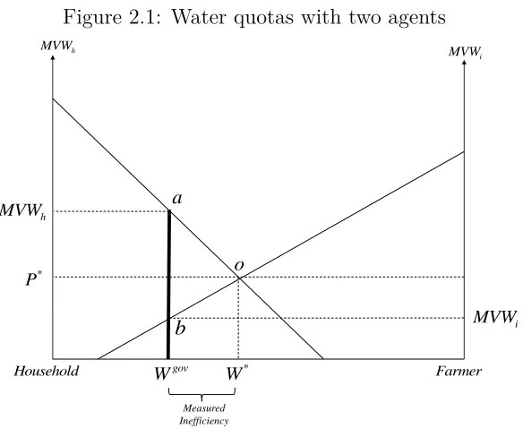
The usual benefits of a market mechanism are illustrated in Figure 2.1. Assume
a closed economy with only two water users. The total water resource is quantity
¯
W, and a social planner allocates Wgov to the household, and ¯W −Wgov to the
farmer. Furthermore, water trade is prohibited. However, this allocation is clearly not
optimal, because the marginal values of water are not equalized, M V Wh > M V Wi.
When water trade is enabled, the household benefits from buying additional units
of water, while the farmer benefits from selling some of his water rights. The
discrep-ancy between the initial administrative allocation and the market allocation is the
Figure 2.1: Water quotas with two agents
a
h
MVW
b
o
Household Farmer
* P
h
MVW
i
MVW
* W
i
MVW
Measured Inefficiency gov
W
Note: Total water ¯W is allocated by the government. Household is allocated water quantityWgov, while farmers
are allocated ¯W−Wgov.Areaaobis the dead weight loss from inefficient water allocation. The potential secondary
water market is the volume|Wgov−W∗|, a proxy for inefficiency.
the quantity traded within this secondary water market is used as a proxy to indicate
the level of inefficient allocation.3
2.2.1
A simplified trade model with water inputs
To describe the model that is used in this paper, consider a simplified closed economy.
Firmi∈N produces a single final goodYi ∈y, using a differentiable constant returns
to scale production functionfi(Li, Wi) that uses labor and water inputs, respectively.
Output prices and wages are pi, pL∈p, respectively.
A representative household h∈H has a rational and locally non-satiated
prefer-ence relation, with a continuous utility function U(y). It consumes final goods Yi,
and waterWh ∈y, and is endowed with a fixed supply of labor ¯Land water ¯W.
The government, which is not explicitly modeled, holds the property rights of
water, and assigns a different increasing block tariff (IBT) for each type of water
[image:32.612.182.474.77.316.2]user, i.e., firms and households pay pW,i, pW,h ∈ p, respectively. However, unlike in
the paper by Diao and Roe (2003), water users are not bound by the water quota
allotted to them. They can, in general, obtain as much water as they desire by paying
increasingly higher prices, within the IBT framework.
Following Mathiesen (1985) and Rutherford (1995, 1999), I set up an Arrow–Debreu
equilibrium as a mixed complementarity problem (MCP). A complementarity
con-straint enforces that two variables are complementary to each other, i.e., that the
following conditions hold for scalar variables x and y: x·y = 0, x≥ 0, y≥ 0. This
condition is compactly expressed as 0≤x⊥y≥0.4
Given the above, ∀i, the firm’s profit maximization problem is to choose labor
and water demands, Li and Wi, so as
Max
Li,Wi≥0
πi(Li, Wi) =pifi(Li, Wi)−pLLi−pW,iWi (2.1)
The disposable income a household is M = pLL¯ +pW,hW¯h +PNi pW,iW¯i, which
includes income from wages, and water charge fees that are collected by the water
authority and transferred to the household. W¯i and ¯Wh denote the administrative
water allocation.5
The household’s utility maximization problem is to choose consumption of goods
and water, Yi and Wh, so as to
Max
Yi,Wh≥0
U(Yi,· · · , YN, Wh) s.t. M ≥ N X
i
piYi+pW,hWh (2.2)
Focusing on water, the first order conditions must be satisfied so that the marginal
4Intuitively, a complementarity constraint is a way to model a constraint that is combinatorial in nature since, for example, the complementary conditions imply that either xor y must be 0 (both may be 0 as well).
5Note that in the initial administrative allocation,W
h= ¯Wh, and could be netted out from both
value of water (M V W) equals the real water price.
M V Wi =
∂fi(·)
∂Wi
≤ pW,i
pi
⊥ Wi ≥0, ∀i (2.3)
M V Wh =
∂U (·)
∂Wh
≤ pW,h
pU
⊥ Wh ≥0 (2.4)
There are three types of weak inequality conditions that must be satisfied in this
general equilibrium model: (i) zero profit, (ii) market clearance, and (iii) income
balance, each associated with three non-negative variables, i.e., y∗ ≥ 0, p∗ ≥ 0 and
M∗ ≥0, respectively.
I define the unit cost function asci =Ci(pL, pW,i, Yi = 1), and the unit expenditure
function of the household ase=E(pi, pW,h, U = 1). Finally, using Shephard’s lemma,
the demands for inputs by the producers, and demand for final goods and water by
the household are summarised by the following weak inequalities, ∀i:
Zero profit conditions: 0≤ci−pi ⊥ Yi ≥0 (2.5)
0≤e−pU ⊥ U ≥0 (2.6)
Market clearing conditions: 0≤Yi−
∂e ∂pi
·U ⊥ pi ≥0 (2.7)
0≤W¯h−
∂e ∂pW,h
·U ⊥ pW,h ≥0 (2.8)
0≤U − M
pU
⊥ pU ≥0 (2.9)
0≤L¯−
N X i=1
∂ci
∂pL
·Yi ⊥ pL≥0 (2.10)
0≤W¯i−
∂ci
∂pW,i
·Yi ⊥ pW,i ≥0 (2.11)
Income balance: M =pLL¯+pW,hW¯h+
N X i=1
pW,iW¯i ⊥ M ≥0 (2.12)
2.2.2
Secondary water market
As described in Figure 2.1 and Equations (2.3) and (2.4), assume that at the initial
administrative allocation with restricted water trade, pW,i
pi = M V Wi < M V Wh =
pW,h
pU , i.e., the household has a higher marginal value of water than firm i. When
water trade is allowed, the household would prefer to buy water from firmi (and the
firm prefers to sell), up to a point where M V Wi =M V Wh.
More generally, water users can be buyers or sellers, and having M = N +H
water users leads to M2 trade configurations,6 with ψ
mn being the relative marginal
value. If user m∈M is a buyer, and user n ∈M is a seller, a possible trade channel
is when M V Wm
M V Wn =ψmn >1; otherwise, it cannot be a possible trade channel. This is
summarise by
M V Wm
M V Wn
=
ψmn >1 possible trade channel
ψmn ≤1 not possible
(2.13)
These conditions, therefore, limit the number of configurations to only T = M(M2−1)
possible trade channels, witht∈T being one specific channel. (Section 2.3.4 discusses
how the marginal values of water are estimated, and Table 2.3 provides a concrete
example for Israel.)
Thus, when water trade is enabled, the units of water, γt, that are transferred
between seller n and buyer m are measured by
0≤γt⊥pW,n,t−(1−)pW,m,t≥0, ∀t (2.14)
with pW,n,t and pW,m,t being the water market prices for the seller and buyer,
re-spectively. For computational purposes, →0 is a small number to ’help’ the solver
with slack activities, thus avoiding the problem of infinite solutions,i.e.,a degenerate
model.7
There are various combinations (scenarios) of activating and deactivating water
trade channels, e.g., activating each channel separately, or all together. Therefore,
each of the t ∈ T channels has a binary action (designed by the scenario); active or
not-active, {A,N A} ∈ Action. There are {tA, tN A} ∈ T channels, {iA, iN A} ∈ N
firms, and {hA, hN A} ∈H households, that are active or not-active, respectively.8
Finally, for a set of actions, the market clearing conditions (2.8) and (2.11) are
replaced with
0≤WA¯ − ∂eA
∂pW,hA
·UA+X
iA
∂ciA
∂pw,iA
·YiA ⊥ pW =pW,hA =pW,iA ≥0 (2.15)
0≤W¯iN A −
∂ciN A
∂pW,iN A
·YiN A ⊥ pW,iN A ≥0 (2.16)
0≤W¯hN A−
∂eN A ∂pW,hN A
·UN A ⊥ pW,hN A ≥0 (2.17)
Equation (2.15) states that the supply of traded water, ¯WA, will equal the demand
for traded water, provided that water prices equalize within the secondary water
market. Equations (2.16) and (2.17) reflect cases in which some water users are
prohibited from trade, and have user-specific water prices and quotas.9
7To insures that when multiple t channels are opened (active), only net transfers of water is considered. For example, a case of infinite solutions is when a first user sells to the second, the second sells to the third, but the first also sells to the third. By adding , the solution is limited to one (possible) case where, for example, the first sells to the second and to the third, while deactivating the second selling to the third.
8In other words, a water user willnot trade because it is either his own choice or it isblocked. 9Here, there is onlyonerepresentative household. Equation (2.17) is a case where the household is blocked from trading, and therefore ∂p∂eA
W,hA
·UA= 0 in Equation (2.15). Extending the analysis to
2.3
The applied general equilibrium model and the
data
In order to adequately represent the actual empirical Israeli economy, the general
equilibrium model that was discussed in the previous section is extended. The
follow-ing will describe the main features of the applied model and of the data used. The
full analytical model is discussed in more detail in Section 3.4.10
Table 2.1 presents key water figures for 2006. Roughly 68% of the total supply of
water in Israel is potable water, of which there are four main users. Approximately
39% of potable water is consumed by the agricultural sector, 6% by the manufacturing
sector, 16% by the service sector, and 39% by private households.11
The use of non-potable water,i.e., salinized, contaminated, sewage effluents, flood,
brackish water, etc., has increased in the past two decades, due to growing pressures
on the supply of water, and improvements in technology and infrastructure.
Approx-imately 95% of it is used by the agricultural sector, and the rest by the manufacturing
sector.
The applied small open economy is aggregated into three main production sectors:
agricultural, manufacturing, and services, and one representative household. The
government is not explicitly modeled, but its actions are manifested through the
initial water allocation, i.e., quota and increasing block tariff (IBT) assignments to
water users.
Table 2.1: Key water figures in Israel (2006)
Potable Water Non-Potable Water
User Mil.
Cubic
Metersa
% of
Total
Expenditure
(mil. NIS)b
Marginal
Value
Waterc
Mil.
Cubic
Metersa
% of
Total
Expenditure
(mil. NIS)b
Agriculture 519 39 768 1.48 589 95 474
Manufacturing 84 6 209 2.49 30 5 24
Services 213 16 833 5.15
Household 524 39 1,889 4.85
Total 1,341 100% 619 100%
% Total Water 68% 32%
Source: a The Water and Sewage Authority, Israel. b Own Calculation: water quantity times relevant price band.
c From the Water Authority 2006 price plan, with assumptions discussed in Section 2.3.4.
2.3.1
Production
Each of the three production sectors uses the following five inputs: labor, capital,
intermediate goods, potable water, and non-potable water.12 The production function
is setup as a four-level nested constant elasticity of substitution (CES) structure,
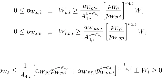
which simplifies the calibration procedure and captures the different substitution
elasticities for pairs of inputs. Some of the main assumptions are the following:
First, the model is calibrated for a short-to-medium time horizon, which affects the
assumptions that are made on factor mobility. Within a time frame of three to four
years, land inputs are relatively rigid because of soil type, location, infrastructure,
and legislative constraints (Hertel, 2002). Here, because capital includes land, capital
is also highly rigid, and is assigned as a sector specific input. This is especially true
for the agricultural sector.
Second, in order to capture the user specific characteristics of water, sector
spe-cific output-supply-price elasticities and water-demand-price elasticities are used to
calibrate for the unknown substitution elasticities. These are summarized in Table
2.2, which are the mid-values from empirical papers. The agricultural sector has
Table 2.2: Output-supply-price and demand-price elasticities
Output
Supply
Elasticitya
Water
Demand
Elasticitya
Potable/Non-Potable
Substitutionb
Agricultural 0.8 -0.7 1.1
Manufacturing 3.0 -0.7 1.1
Services 3.0 -0.1
Household -0.1
Source: aApproximate mid-values reported in various papers. bIsrael Water Authority
Note: The above values, together with the cost share from the social accounting matrix, calibrate the input substitution
elasticities for households and sectors. (See Section 3.4.)
a relatively inelastic supply price elasticity of 0.8, partly due to high land rigidity.
Non-agricultural sectors have an elastic supply price elasticity of 3.0. Furthermore,
both the agricultural and manufacturing sector have a water demand price elasticity
of -0.7, while the residential water demand price elasticity is -0.1, i.e., service sectors
and households.13 As in many applied models, intermediate inputs are assumed to
enter in fixed proportions (Leontief technology). Finally, the substitution elasticity
between potable and non-potable water is assumed to be 1.1.14
Third, labor inputs freely migrate between the various sectors, and have a global
wage level, pL. Finally, in the benchmark, water inputs are allotted to users and are
non-tradable, and water prices,pW,i, are sector specific. As discussed in Section 2.2.2,
when water-trade is allowed, water is reassigned as a global input, and trade occurs
until the market clears. Water prices change sufficiently to drive water marginal
values to equalize between users.
13Sections 3.5 and 3.6 provide a detailed description of the empirical literature and assumptions behind these values, and explain the calibration method from the known elasticities and cost share to the unknown substitution elasticities within the production and utility functions.
2.3.2
Household
The small open economy has one representative household that is endowed with labor,
capital, and water resources, ¯L, ¯K, ¯W, respectively. Tax revenues are transferred to
the household, including positive (negative) transfers of income to cover balance of
payments, bop. Income is
M =PW,hW¯h+ n X i=1
PLL¯i+PK,iK¯i+PW,p,iW¯p,i+PW,np,iW¯np,i+τi+bopi
(2.18)
and utility is derived by consuming potable water and final goods, using a two-level
nest CES-Cobb Douglas function. Table 2.2 reports that the residential water demand
price elasticity is -0.1, which I use to calibrate the unknown substitution elasticity
between the demand for water and a bundle of final consumption goods.
2.3.3
General assumptions in the model
Two assumptions are made in the model. First, in order to properly compare the
welfare effects between the benchmark and the counter-factual scenarios, and because
this is a static model, the balance of payments (BOP) is fixed to the year specific
levels. Otherwise, it would not make sense to allow for policy experiments to increase
the trade deficit and thus increase welfare, at the expense of foreign borrowing. Such
a situation would be misleading because in a fully dynamic model, borrowing will
have to be paid back at some point.15
Second, having increasing block water tariffs usually means that higher block
tariff users subsidize lower block tariff users. Here, however, the model is simplified
by aggregating many different users to only four main groups, each having one water
price. Disaggregating users into further subgroups is possible, but would require a
more detailed social accounting matrix. In this model it is therefore assumed that all
users within a group have the same size and preferences, or that they have already
traded water internally between themselves.
2.3.4
Data and marginal value of water
The data used in the model is obtained from the Use-Supply tables published by the
Israeli Central Bureau of Statistics (CBS) for 1995, 2000, 2004, 2005 and 2006.
(Sim-ilar data for 2007 is not yet available.) The data include sector outputs and inputs,
household consumption and trade balance, as well as levels of taxes and subsidies.
From these, social accounting matrices (SAM) are constructed and used to calibrate
the model (Round, 2003). Labour inputs are obtained from the Compensation of
Employees by Industry tables from the Israeli CBS.
The Water Authority assigns increasing block tariff (IBT), whereby consumers pay
progressively higher water prices for each increasing quantity of water consumed.16
Each main user, i.e., agricultural, manufacturing, services, and households, has a
different IBT structure.17
CBS does not report the water sector separately from the electricity sector, and
does not distinguish between potable and non-potable water. Therefore, the
ex-penditure on water has to be estimated by other means, rather than directly from the
Use-Supply tables. Residential water expenditure,i.e., household and service sectors,
are estimated by summing the total water quantity times the relevant tariff band for
each type of residential user.18 Agricultural water expenditure is obtained by
mul-tiplying the quantity of total potable water supply by tariff block A. This method is
similarly used to estimate the expenditure on potable water for manufacturing, and
expenditure on non-potable water, which each have one main water price band.
16But not necessarily higher,e.g., manufacturing has a lower price for water use above the 100% quota.
Water users can obtain as much, or as little, water as they are willing to
pay-for. This means that their marginal value of water (MVW) is equal, or somewhere
below the next tariff block, of the last unit of water. Table 2.1 summarizes the total
monetary expenditure on water, and the estimated marginal value for 2006. Recall
that conservative values are preferred, and that this would increase water trade,e.g.,
by lowering the MVW for farmers and increasing it for households. The following are
the underlying assumptions for the marginal value of water:
Agricultural water quotas were revised in 1989 and the following tariff blocks were
introduced. Tariff A is charged up-to 50% of the quota, tariff B between 50-80%, and
tariff C between 80%-100%. There are two further bands above 100% with lower
prices.19 Since 1989, extensive cuts in potable water quotas have been made, and
most of agricultural users pay tariff A, which is thus assigned as their marginal value
for water.20
Manufacturing sectors have one main tariff up to 100% of the quota, and this is
assigned as the marginal value of water.21
Different service sectors are assigned different tariffs. For example, hospitals and
mikves22 fall under tariff A. Hotels fall under tariff B, while the rest of the service
sectors (e.g., commerce, education, sport, public) fall under tariff C. Public gardens
are charged tariff D. In the model, tariff C is used as the marginal value of water for
service sectors, because it captures 62% of the water used. Public gardens consume
around 25% of water in the service sector, but they do not account for GDP.
Finally, the household price scheme for 2006 includes four tariff blocks. Tariff B
captures around 61% of the total consumed water by households, and is therefore
19The two further blocks are: (1) up-to 10% above the quota, and (2) above 10% above the quota. See Section 3.7.2 of Chapter 3 for further detail.
20From a discussion with the Water Authority. Agricultural water consumption is not published, as it is done with residential consumption. Furthermore, the secondary water market would be smaller if tariff B would have been chosen. When in doubt, the larger, more conservative, secondary water market is preferred.
Table 2.3: Water trade channels: relative MVW for 2006
Buyerm∈M
Agricultural Manufacturing Services Household
Agricultural 1 1.684 3.484 3.283
Sellern∈M Manufacturing 0.594 1 2.069 1.949
Service 0.287 0.483 1 0.942
Household 0.305 0.513 1.061 1
Note: These are the ratio of seller/buyer water marginal value. Divide values from the fifth column in Table 2.1 and
numbers in bold are the possible water trade channels.
chosen as their estimated marginal value of water.23
Table 2.3 is an applied example of the discussion in Section 2.2.2. It shows that
having four main water users in Israel leads to sixteen water trade configurations.
In order to obtain the relative marginal value of water (MVW) for a buyer/seller
ψmn, as in Equation (2.13), divide the marginal values of water for each pair of users
reported in Table 2.1. Values greater than one indicate which water trade channels
are possible, and who would be the sellers and buyers. The six possible channels
are marked in bold in Table 2.3. The service sector, for example, values water by
approximately 3.484 times that of the agricultural sector, and therefore, would buy
from the agricultural sector (not sell).
2.4
Measuring the efficiency of an administrative
water allocation
In this section of the applied model, water is initially allotted administratively to
each of the four users, and water trade is forbidden. Then, in the counter-factual
experiments, trade is allowed and water inputs are re-shuffled until all users have the
same marginal value of water.
Compared to a market allocation, a certain degree of administrative
misalloca-tion is expected. The quesmisalloca-tion is, therefore, how large is the potential secondary
water market likely to be? A large misallocation could indicate a poor administrative
mechanism. It would suggest that a market mechanism may be superior, and that the
government is committing a type II error by maintaining the current administrative
allocation and not introducing a water market.
If, however, the misallocation is rather small, it is unclear which mechanism is
better. Section 2.5, therefore, extends the model and includes the non-marketed
social value. Together, this section and the next contribute to a better assessment of
the most preferable mechanism for Israel.
2.4.1
Results for 2006
The main results, which are: the size of the secondary potable water market, the
welfare gains, and their effect on the nominal water price, are reported in Table 2.4.
The most important outcome is the all-channel-trade scenario, in which the
sec-ondary potable water market is estimated at 80.8 million cubic meters (MCM). This
is approximately 6.0% of the total potable water consumption in Israel in 2006. The
agricultural sector sells 22.5 MCM of potable water to the manufacturing sector, 17.9
MCM to the service sector, and 40.3 MCM to households.
Because the Water Authority practices price discrimination, the secondary water
market clears when nominal water prices rise (or fall) sufficiently to allow the marginal
value of water to equalize for all users (reported in the right hand side of Table 2.4).
In the all-trade scenario, the agricultural water price rises by 22.6%, and falls for
manufacturing, services, and households by 27.2%, 64.8%, and 62.7%, respectively.
This means that in 2006, the market clearing nominal water price (shadow price)
would have been NIS/MC 1.81.
Table 2.4: Model results (2006, % change)
% of Welfare % Change in water prices
Water* total gains Potable water Non-potable
Channel (seller to buyer) MCM potable NIS mill. Agri Indus Serv House water
1. Agriculture to Manufacturing 32.7 2.4 21.5 8.0 -35.9 1.1
2. Agriculture to Services 20.7 1.5 24.9 5.0 -69.8 1.2
3. Agriculture to Household 44.5 3.3 51.0 11.5 -66.0 2.6
4. Manufacturing to Services 9.5 0.7 5.7 17.5 -43.2 0.3
5. Manufacturing to Household 15.5 1.2 8.2 31.9 -32.3 0.6
6. Household to Services 0.7 0.1 0.1 -4.1 1.8 0.0
All Channel Trade 80.8 6.0 86.3 22.6 -27.2 -64.8 -62.7 4.4
(of which)
Manufacturing buys 22.5 1.7
Services buys 17.9 1.3
Household buys 40.3 3.0
Shadow Water Price (All Channel) NIS/CM 1.81
*Total potable consumed, in 2006, was 1340.5 Million Cubic Meters (MCM).
Note: Model’s results for 2006 data. The second column is the quantity of water traded within each channel of the
secondary water market. The third column is the percent of water traded of the total potable water supply in that
year. The fourth column are the welfare gains in New Israeli Shekels (NIS) Million. The right hand section is percent
change of nominal water price from the initial allocation.
the economy such as production levels, sector specific return to capital, wage level
and welfare. Table 2.5 reports the most important of them. These changes might
seem small, but are a result of potable water inputs being only 2% of total input
cost in the agricultural sector, and less than 0.1% for manufacturing and service
sectors. Household expenditure on potable water is only 0.2% of disposable income.24
Therefore, the household utility level (welfare) rises by only 0.01%. This is, however,
equivalent to a 2.3% increase in economic value relative to the size of the water sector,
and approximately 86.3 Million New Israeli Shekels (NIS) in 2006 prices (see fourth
column in Table 2.4). The intuition behind these results is that by allowing for water
trade, water inputs are put to better use, and the production possibility frontier of
Table 2.5: Other key results (2006, % change)
Agriculture Manufacturing
Channel Prod. Price Return on
Capital
Prod. Price Return on
Capital
3. Agr sell to Hh -0.2 0.4 0.13 -0.024 0.14 0.13
All Trade -0.4 0.7 0.13 -0.04 0.15 0.14
Services Other Variables
Prod. Price Return on
Capital
Wage Water Sector
GDP
Price
Non-Potable
3. Agr sell to Hh -0.01 0.13 0.13 0.13 1.4 2.6
All Trade 0.02 0.10 0.13 0.27 2.3 4.4
Note: Model output for 2006 - continued from Table 2.4. Values are percent change from the initial allocation.
the economy moves outwards.
To better understand the mechanism within this general equilibrium model, it
is useful to focus, for example, on channel 3 in Table 2.4 and Table 2.5, where the
agricultural sector sells only to households. In this channel, which has the largest
impact on water trade, the size of the water transfer is around 44.5 MCM. Relative to
the initial administrative prices, market water prices rise by 11.5% for the agricultural
sector, and fall by 66% for households (see Table 2.4 channel 3).
As Table 2.5 reports, agricultural output falls by 0.2%, which raises the
agricul-tural price by 0.4% and raises agriculagricul-tural return on capital by 0.13%. As mentioned
earlier, capital is a sector specific input, and will not have a direct effect on the rest of
the economy. However, when water inputs are transferred to households, this raises
demand for labour within the agricultural sector, and leads to a wage increase across
the whole economy. Indirectly, this raises the cost of production in the other two
sectors, even though they are not involved in the water market. Production levels,
Table 2.6: Values used for sensitivity analysis, 2006
Output Supply Elast. Water Demand Elast.
Sector Min Model Max Min Model Max
Agriculture 0.4 0.8 1.2 -0.1 -0.7 -2
Manufacturing 1 3 5 -0.1 -0.7 -2
Services 1 3 5 -0.01 -0.1 -1
Household -0.01 -0.1 -1
Note: Max. and min. range for supply-price and demand-price elasticities. Bold numbers are the benchmark values.
2.4.2
Sensitivity analysis
Sensitivity analysis was performed on each sector using minimum and maximum
parameters for the various output supply elasticities, and water demand elasticities
(summarized in Table 2.6). These parameters are well above and below the accepted
values that are reported and used in other studies. The results suggest that the model
is well-behaved, and that the main results are robust.
Output supply price elasticity has a negligible effect on the size of the water
market because, as previously mentioned, water accounts for a very small fraction of
the input cost in production. Furthermore, capital is a sector specific input, which
dampens the effect of parameter changes. Experimenting also with capital as a fully
tradable input does not change the size of the secondary water market by any measure
worth reporting.
A larger effect on the secondary water market comes from changing the water
demand elasticities. Using unlikely, extreme, values for both agriculture and
manu-facturing sectors, the potential secondary water market reaches a range of 3.6% to
7.8% of the total potable water supplied. Yet, the outcomes are not significantly
different from the main result of 6%. Changing the water demand elasticities for
res-idential users,i.e., service sectors and households, by an unlikely order of magnitude
of 10, changes the range from 4% to 18% of total potable water. Again, these are