Evaluation of Feature Subset Selection, Feature
Weighting, and Prototype Selection for Biomedical
Applications
Suzanne LITTLE1, Sara COLANTONIO 2, Ovidio SALVETTI2, Petra PERNER1*
1Institute of Computer Vision and Applied Computer Sciences, Germany; 2ISTI-CNR, Pisa, Italy. Email: [email protected]
Received September 15th, 2009; revised October 9th, 2009; accepted October 21st, 2009.
ABSTRACT
Many medical diagnosis applications are characterized by datasets that contain under-represented classes due to the fact that the disease is much rarer than the normal case. In such a situation classifiers such as decision trees and Naïve Bayesian that generalize over the data are not the proper choice as classification methods. Case-based classifiers that can work on the samples seen so far are more appropriate for such a task. We propose to calculate the contingency table and class specific evaluation measures despite the overall accuracy for evaluation purposes of classifiers for these specific data characteristics. We evaluate the different options of our case-based classifier and compare the perform-ance to decision trees and Naïve Bayesian. Finally, we give an outlook for further work.
Keywords: Feature Subset Selection, Feature Weighting, Prototype Selection, Evaluation of Methods, Prototype-Based Classification, Methodology for Prototype-Based Classification, CBR in Health
1. Introduction
Many medical diagnosis applications are characterized by datasets that contain under-represented classes due to the fact that the disease is much rarer than the normal case. In such a situation classifiers such as decision trees and Naïve Bayesian that generalize over the data are not the proper choice as classification methods. Decision trees tend to over-generalize the class with the most ex-amples while Naïve Bayesian requires enough data for the estimation of the class-conditional probabilities. Case-based classifiers that can work on the samples seen so far are more appropriate for such a task.
A case-based classifier classifies a new sample by finding similar cases in the case base based on a proper similarity measure. A good coverage of the casebase, the right case description and the proper similarity are the essential functions that enable a case-based classifier to perform well.
In this work we studied the behavior of a case-based classifier based on different medical datasets with dif-ferent characteristics from the UCI repository [1]. We chose datasets where one or more classes were heavily under-represented compared to the other classes as well as datasets having more or less equally distributed sam-ples for the classes for comparison purposes.
The case-based classifier has several options for im-proving its performance that can be chosen independ-ently or in combination. Currindepend-ently available options in our case-based classifier are: k-value for the closest cases; feature subset selection (FS); feature weight learning (FW); and prototype selection (PS). To con-clusively determine which combination of options is best for the current problem is non-obvious and time- consuming and we hope to develop with our study a methodology that assists a user in designing and refin-ing our case-based classifiers. We observe the influ-ence of the different options of a case-based classifier and report the results in this paper. Our study is an on-going study; we also intend to investigate other op-tions in casebase maintenance.
2. Case-Based Classifiers
A case-based classifier classifies a sample according to the cases in a case base and selects the most similar case as output of the classifier. A proper similarity measure is necessary to perform this task but in most applications no a-priori knowledge is available that suggests the right similarity measure. The method of choice for selecting the proper similarity measure is therefore to apply a sub-set of the numerous statistically derived similarity meas-ures to the problem and to select the one that performs best according to a quality measure such as the classifi-cation accuracy. The other choice is to automatically build the similarity metric by learning the right attributes and attribute weights. We chose the latter as one option to improve the performance of our classifier.
When people collect samples to construct a dataset for a case-based classifier it is useful to select prototypical examples from the samples. Therefore, a function is needed to perform prototype selection and to reduce the number of examples used for classification. This results in better generalization and a more noise tolerant classi-fier. An expert is also able to select prototypes manually. However, this can result in bias and possibly duplicates of prototypes and may therefore cause inefficiencies. Therefore, a function to assess a collection of prototypes and identify redundancy is useful.
Finally, an important variable in a case-based classifier is the value used to determine the number of closest cases and the final class label.
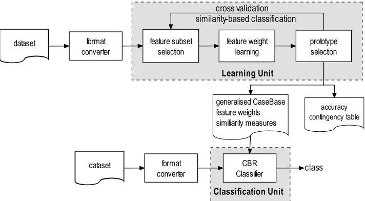
Consequently, the design-options available for impro- ving the performance of the classifier are prototype se-lection, feature-subset sese-lection, feature weight learning and the ‘k’ value of the closest cases (see Figure 1).
We choose a decremental redundancy-reduction algo-rithm proposed by Chang [2] that deletes prototypes as long as the classification accuracy does not decrease. The feature-subset selection is based on the wrapper approach [3] and an empirical feature-weight learning method [4] is used. Cross validation is used to estimate the classifi-cation accuracy. A detailed description of our classifier ProtoClass is given in [6. The prototype selection, the feature selection, and the feature weighting steps are performed independently or in combination with each other in order to assess the influence these functions have on the performance of the classifier. The steps are per-formed during each run of the cross-validation process. The classifier schema shown in Figure 1 is divided into the design phase (Learning Unit) and the normal classi-fication phase (Classiclassi-fication Unit). The classiclassi-fication phase starts after we have evaluated the classifier and determined the right features, feature weights, the value for ‘k’ and the cases.
Our classifier has a flat case base instead of a hierar-chical one; this makes it easier to conduct the evalua-tions.
2.1 Classification Rule
This rule [5] classifies x in the category of its closest case. More precisely, we call xnx1,x2,…,xi,…xn a closest case to x if mind x x
i,
d x x
n,
, where i=1,2,…,n.The rule classifies x into category Cn, where xn is the closest case to x and xn belongs to class Cn.
In the case of the k-closest cases we require k-samples of the same class to fulfill the decision rule. As a distance measure we use the Euclidean distance.
dataset format converter
feature subset selection
feature weight learning
prototype selection
generalised CaseBase feature weights similiarity measures
Learning Unit similarity-based classificationcross validation
CBR Classifier
Classification Unit
class dataset format
converter
[image:2.595.121.477.499.695.2]accuracy contingency table
2.2 Prototype Selection by Chang’s Algorithm For the selection of the right number of prototypes we used Chang’s algorithm [2] The outline of the algorithm can be described as follows: Suppose the set T is given as T={t1,…,ti,…,tm} with ti as the i-th initial prototype. The principle of the algorithm is as follows: We start with every point in T as a prototype. We then successively merge any two closest prototypes t1 and t2 of the same
class to a new prototype t, if merging will not downgrade the classification of the patterns in T. The new prototype t may simply be the average vector of t1 and t2. We
con-tinue the merging process until the number of incorrect classifications of the pattern in T starts to increase.
Roughly, the algorithm can be stated as follows: Given a training set T, the initial prototypes are just the points of T. At any stage the prototypes belong to one of two sets-set A or set B. Initially, A is empty and B is equal to T. We start with an arbitrary point in B and initially as-sign it to A. Find a point p in A and a point q in B, such that the distance between p and q is the shortest among all distances between points of A and B. Try to merge p and q. That is, if p and q are of the same class, compute a vector p* in terms of p and q. If replacing p and q by p*
does not decrease the recognition rate for T, merging is successful. In this case, delete p and q from A and B, re-spectively, and put p* into A, and repeat the procedure
once again. In case that p and q cannot be merged, i.e. if either p or q are not of the same class or merging is un-successful, move q from B to A, and repeat the procedure. When B empty, repeat the whole procedure by letting B be the final A obtained from the previous cycle, and by resetting A to be the empty set. This process stops when no new merged prototypes are obtained. The final proto-types in A are then used in the classifier.
2.3 Feature-Subset Selection and Feature Weighting
The wrapper approach [3] is used for selecting a feature subset from the whole set of features and for feature weighting. This approach conducts a search for a good feature subset by using the k-NN classifier itself as an evaluation function. By doing so the specific behavior of the classification methods is taken into account. The leave-one-out cross-validation method is used for esti-mating the classification accuracy. Cross-validation is especially suitable for small data set. The best-first search strategy is used for the search over the state space of possible feature combination. The algorithm termi-nates if no improved accuracy over the last k search states is found.
The feature combination that gave the best classifica-tion accuracy is the remaining feature subset. We then try to further improve our classifier by applying a feature- weighting tuning-technique in order to get real weights for the binary weights.
The weights of each feature wi are changed by a
con-stant value, : wi:=wi±. If the new weight causes an
improvement of the classification accuracy, then the weight will be updated accordingly; otherwise, the weight will remain as is. After the last weight has been tested, the constant will be divided into half and the procedure repeated. The process terminates if the differ-ence between the classification accuracy of two interac-tions is less than a predefined threshold.
3. Classifier Construction and Evaluation
Since we are dealing with small sample sets that may sometimes only have two samples in a class we choose leave one-out to estimate the error rate. We calculate the average accuracy and the contingency table (see Table 1) showing the distribution of the class-correct classified samples as well as the distribution of the samples classi-fied in one of the other classes. From this table we can derive a set of more specific performance measures that had already demonstrated their advantages in the com-parison of neural nets and decision trees [3] such as the classification quality (also called the sensitivity and specificity in the two-class problem).The true class distribution within the data set and the class distribution after the samples have been classified as well as the marginal distribution cij are recorded in the
fields of the table. The main diagonal is the number of cor-rectly classified samples. From this table, we can calculate parameters that describe the quality of the classifier.
The correctness or accuracy p (Equation 1) is the number of correctly classified samples relative to the number of samples. This measure is the opposite to the error rate.
m
i m
j ij c m
i cii p
1 1
1 (1)
The class specific quality pki (Equation 2) is the num-ber of correctly classified samples for one class i relative to all samples of class i and the classification quality pti (Equation 3) is the number of correctly classified sam- ples of class i relative to the number of correctly and falsely classified samples into class i:
Table 1. Contingency table
True Class Label (assigned by expert)
1 i … m pki
1 c11 ... ... c1m
i ... cii ... ...
… ... ... ... ...
m cm1 ... ... cmm Assigned
Class Label (by Classifier)
m
j ji ii ki
c c p
1
(2)
m
j ji ii ki
c c p
1
(3)
These measures allow us to study the behavior of a classifier according to a particular class. The overall error rate of a classifier may look good but we may find it un-acceptable when examining the classification quality pti
for a particular class.
We also calculate the reduction rate, that is, the num-ber of samples removed from the dataset versus the number of samples in the case base.
The classifier provides several options, prototype- se-lection, feature subset sese-lection, and feature weighting, which can be chosen combinatorially. We therefore per-formed the tests on each of these combinations in order to understand which function must be used for which data characteristics. Table 2 lists the various combina-tions.
4. Datasets and Methods for Comparison
A variety of datasets were chosen from the UCI reposi-tory [1]. The IRIS and E.coli datasets are presented here as representative of the different characteristics of the datasets. Space constraints prevent the presentation of other evaluations in this paper.The well-known, standard IRIS Plant dataset consists of sepal and petal measurements from specimens of IRIS plants and aims to classify them into one of three species. The dataset consists of 3 equally distributed classes of 50 samples each with 4 numerical features. One species (setosa) is linearly separable from the other two, which are not linearly separable from each other. This is a sim-ple and frequently applied dataset within the field of pat-tern recognition.
[image:4.595.307.538.101.181.2]The E. coli dataset aims to predict the cellular local-ization sites of proteins from a number of signal and laboratory measurements. The dataset consists of 336 instances with 7 numerical features and belonging to 8 classes. The distribution of the samples per class is
Table 2. Combinations of classifier options for testing
Test Feature Subset Selection Weighting Feature Prototype Selection
1 1
2 1
3 1
4 1 2 3 5 2 3 1
highly disparate (143/77/2/2/35/20/5/52).
The Wisconsin Breast Cancer dataset consists of visual information from scans and provides a classification problem of predicting the class of the cancer as either benign or malignant. There are 699 instances in the data-set with a distribution of 458/241 and 9 numerical fea-tures.
For each dataset we compare the overall accuracy generated from:
1) Naïve Bayesian, implemented in Matlab;
2) C4.5 decision tree induction, implemented in DE-CISION MASTER [12];
3) k-Nearest Neighbor (k-NN) classifier, implemented in Weka [11] with the settings “weka.classifiers.lazy.IBk -K k-W 0-A” weka.core.neighboursearch. LinearNN-Search-A weka.core.EuclideanDistance” and the k- Nearest Neighbor (k-NN) classifier implemented in Mat-lab (Euclidean distance, vote by majority rule).
4) case-based classifier, implemented in ProtoClass (described in Section 2) without normalization of features.
Where appropriate, the k values were set as 1, 3 and 7 and leave-one-out cross-validation was used as the eva- luation method. We refer to the different “implementa-tions” of each of these approaches since the decisions made during implementation can cause slightly different results even with equivalent algorithms.
5. Results
[image:4.595.112.483.631.719.2]The results for the IRIS dataset are reported in Tables 4-6. Table 4 shows the results for Naïve Bayes, decision tree induction, k-NN classifier done with Weka implementa-tion and the result for the combinatorial tests described in Table 2 with ProtoClass. As expected, decision tree in-duction performs well since the data set has an equal data distribution but not as well as Naïve Bayes.
Table 3. Dataset characteristics and class distribution
No.
Samples Features No. ClassesNo. Class Distribution
setosa versicolor virginica
IRIS 150 4 3
50 50 50
cp im imL imS imU om omL pp
E.Coli 336 7 8 143 77 2 2 35 20 5 52
benign malignant
Wisconsin 699 9 2
Table 4. Overall accuracy for IRIS dataset using leave-one-out
k Naïve
Bayes Deci-sion
Tree
kNN
Proto-Class Feature Subset Feature Weighting Prototype Selection FS+ FW+ PS
PS+ FS+ FW
1 95.33 96.33 95.33 96.00 X X 96.00 96.00 96.33 3 na na 95.33 96.00 96.33 96.33 96.00 96.33 96.00 7 na na 96.33 96.67 X 96.00 96.00 96.33 96.00
Table 5. Contingency table for k=1,3,7 for the IRIS dataset and protoclass
IRIS setosa versicolor Virginica
k 1 3 7 1 3 7 1 3 7
setosa 50 50 50 0 0 0 0 0 0
versicolor 0 0 0 47 47 46 3 3 4
virginica 0 0 0 3 3 1 47 47 49
[image:5.595.59.287.309.376.2]Classification quality 100 100 100 94 94 97.87 94 94 92.45 Class specific quality 100 100 100 94 94 92 94 94 98
Table 6. Class distribution and percentage reduction rate of IRIS dataset after prototype selection
Iris- sertosa
Iris- versicolor
Iris- virginica
Reduction Rate in %
orig 50 50 50 0.00
k=1 50 49 50 0.67
k=3 50 49 50 0.67
k=7 50 48 50 1.33
[image:5.595.58.541.405.468.2]In general we can say that the accuracy does not sig-nificantly improve when using feature subset selection, feature weighting and prototype selection with Proto-Class. In case of k=1 and k=7 the feature subset remains the initial feature set. This is marked in Table 4 by an “X” indicating that no changes were made in the design phase and the accuracy is the same as for the initial clas-sifier. This is not surprising since the data base contains
Table 7. Overall accuracy for E. coli dataset using leave-one-out
k Naïve Bayes Decision Tree
Weka Near-est Neighbour
Matlab
knn ProtoClass
Feature Subset
(FS)
Feature Weighting
(FW)
Prototype Selection
(PS)
FS+FW+ PS
PS+FS+ FW
1 86.01 66.37 80.95 80.06 81.25 80.95 83.04 80.65 82.44 80.95
3 na na 83.93 84.26 84.23 85.12 84.23 82.74 83.93 82.74
[image:5.595.59.540.493.664.2]7 na na 86.40 86.31 87.20 87.20 86.31 86.61 85.42 86.61
Table 8. Combined contingency table for k=1,3,7 for the E. coli dataset and protoClass
cp im imL imS imU Om omL pp
k 1 3 7 1 3 7 1 3 7 1 3 7 1 3 7 1 3 7 1 3 7 1 3 7
cp 133 139 140 4 0 0 0 0 0 0 0 0 0 0 0 0 0 0 0 0 0 6 4 3
im 3 4 3 56 60 60 1 0 0 1 0 0 15 12 11 0 0 0 0 0 0 1 0 3
imL 0 0 0 1 1 1 0 0 0 0 0 0 0 0 0 0 0 0 1 1 1 0 0 0
imS 0 0 0 0 0 0 0 0 0 0 0 0 1 1 1 0 0 0 0 0 0 1 1 1
imU 1 1 1 15 16 12 0 0 0 0 0 0 19 17 22 0 1 0 0 0 0 0 0 0
om 0 0 0 0 0 0 0 0 0 0 0 0 1 0 0 16 17 17 0 1 1 3 2 2
omL 0 0 0 0 0 0 0 0 0 0 0 0 0 0 0 0 0 0 5 5 5 0 0 0
pp 5 4 4 1 1 1 0 0 0 0 0 0 0 0 0 2 2 0 0 0 0 44 45 47
pki 93.66 93.92 94.59 72.73 76.92 81.08 0.00 0 0 0.00 0 0 52.78 56.67 64.71 88.89 85.00 100.00 83.33 71.43 71.43 80.00 86.54 83.93
pti 93.01 97.20 97.90 72.73 78.95 77.92 0.00 0.00 0.00 0.00 0.00 0.00 54.29 48.57 62.86 80.00 85.00 85.00 100.00 100.00 100.00 84.62 86.54 90.38
only 4 features which are more or less well-distinguished. In case of k=3 a decrease in accuracy is observed al-though the stopping criteria for the methods for feature subset selection and feature weighting require the overall
Table 9. Learnt weights for E. coli dataset
k f1 f2 f3 f4 f5 f6 f7
1 0.5 1 1 1 0.75 1.5 1
3 1.5 0 1 1 1 1 1
7 0.75 0.5 1 1 1 1 1
final overall accuracy. Prototype selection where k=7 demonstrates the same behavior. This shows that the true accuracy must be calculated based on cross validation and not simply based on the design data set.
[image:6.595.89.503.169.239.2]We expected that feature subset selection and feature
Table 10. Class distribution and percentage reduction rate of E. coli dataset after prototype selection
cp im imL imS imU om omL pp Reduction
rate in %
orig 143 77 2 2 35 20 5 52 0.00
k=1 140 73 2 2 34 20 5 49 3.27
k=3 142 72 2 2 31 20 5 52 2.97
k=7 142 76 2 2 32 20 5 50 2.08
weighting would change the similarity matrix and there-fore we believed that prototype selection should be done afterwards. As shown in the Table 4 in case of k=3 we do not achieve any improvement in accuracy when running PS after the feature options. However, when conducting PS before FS and FW, we see that FS and FW do not have any further influence on the accuracy. When com-bining FS/FW/PS, the final accuracy was often the same as the accuracy of the first function applied. Therefore, prototype selection prior to feature subset selection or feature weighting seems to provide a better result.
The contingency table in Table 5 provides a better un-derstanding in respect to what is happening during clas-sification. The table shows which samples are misclassi-fied according to what class. In case of k=1 and k=3 the misclassification is more equitably distributed over the classes. If we prefer to accurately classify one class we might prefer k=7 since it can better classify class “vir-ginica”. The domain determines what requirements are expected from the system.
Table 6 shows the remaining sample distribution ac-cording to the class after prototype selection. We can see that there are two or three samples merged for class “ver-sicolor”. The reduction of the number of samples is small (less than 1.4% reduction rate) but this behavior fits our expectations when considering the original data set. It is well known that the IRIS dataset is a pre-cleaned dataset.
Table 7 lists the overall accuracies for the different approaches using the E. coli dataset. Naïve Bayesian
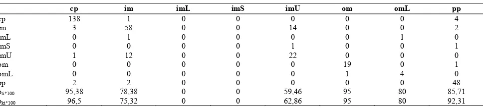
shows the best overall accuracy while decision tree in-duction exhibits the worst one. The result for Naïve Bayesian is somewhat curious since we have found that the Bayesian scenario is not suitable for this data set. The true class conditional distribution cannot be estimated for the classes with small sample number. Therefore, we consider this classifier not to be applicable to such a data set. That it shows such a good accuracy might be due to the fact that the classifier can classify excellently the classes with large sample number (e.g., cp, im, pp) and the misclassification of samples from classes with a small number do not have a big impact on the overall accuracy. Although previous evaluations have used this data to demonstrate the performance of their classifier on the overall accuracy (for example in [11,12]) we suggest that this number does not necessarily reflect the true per-formance of the classifier. It is essential to examine the data characteristics and the class-specific classification quality when judging the performance of the classifier.
As in the former test, the k-NN classifier of Weka does not perform as well as the ProtoClass classifier. The same is true for the knn-classifier implemented in Matlab. The best accuracy is found surprisingly for k=7 but the contingency table (Table 8) confirms again that the classes with small sample number seem to have low im-pact on overall accuracy.
[image:6.595.59.543.610.719.2]Feature subset selection works on the E. coli dataset. One or two features drop out but the same observations as of the IRIS data set are also true here. We can see an
Table 11. Contigency table for E. coli dataset and Naïve Bayes Classifier
cp im imL imS imU om omL pp
cp 138 1 0 0 0 0 0 4
im 3 58 0 0 14 0 0 2
imL 0 1 0 0 0 0 1 0
imS 0 0 0 0 1 0 0 1
imU 1 12 0 0 22 0 0 0
om 0 0 0 0 0 19 0 1
omL 0 0 0 0 0 1 4 0
pp 2 2 0 0 0 0 0 48
pti*100 95,38 78,38 0 0 59,46 95 80 85,71
Table 12. Contigency table for E. coli dataset and Matlab knn Classifier
T O T
k 1 3 7 1 3 7 1 3 7 1 3 7 1 3 7 1 3 7 1 3 7 1 3 7
cp 133 139 140 4 0 0 0 0 0 0 0 0 0 0 0 0 0 0 0 0 0 6 4 3 14
im 3 4 3 56 60 60 1 0 0 1 0 0 15 12 11 0 0 0 0 0 0 1 0 3 7
imL 0 0 0 1 1 1 0 0 0 0 0 0 0 0 0 0 0 0 1 1 1 0 0 0
imS 0 0 0 0 0 0 0 0 0 0 0 0 1 1 1 0 0 0 0 0 0 1 1 1
imU 1 1 1 15 16 12 0 0 0 0 0 0 19 17 22 0 1 0 0 0 0 0 0 0 3
om 0 0 0 0 0 0 0 0 0 0 0 0 1 0 0 16 17 17 0 1 1 3 2 2 2
omL 0 0 0 0 0 0 0 0 0 0 0 0 0 0 0 0 0 0 5 5 5 0 0 0
pp 5 4 4 1 1 1 0 0 0 0 0 0 0 0 0 2 2 0 0 0 0 44 45 47 5
pti 0,94 0,94 0,95 0,73 0,77 0,81 0,00 0,00 0,00 0,00 0,00 0,00 0,53 0,57 0,65 0,89 0,85 1,00 0,83 0,71 0,71 0,80 0,87 0,84
pki 0,93 0,97 0,98 0,73 0,78 0,78 0,00 0,00 0,00 0,00 0,00 0,00 0,54 0,49 0,63 0,80 0,85 0,85 1,00 1,00 1,00 0,85 0,87 0,90
omL pp
cp im imL imS imU om
3 7 2 2 5 0 5 2
50.00 70.00 90.00 110.00
143 77 2 2 35 20 5 52
cp im imL imS imU om omL pp
Classes and Number of Samples
C
lassi
fi
ca
ti
o
n
Q
u
al
it
y Naive Bayes
[image:7.595.132.463.414.556.2]Math knn 1 Math knn 3 Math knn 7 Proto k 1 Proto k 3 Proto k 7
Figure 2. Classification quality for the best results for Naïve Bayes, Math knn, and Protoclass
50.00 70.00 90.00 110.00
143 77 2 2 35 20 5 52
cp im imL imS imU om omL pp
Classes and Number of Samples
C
las
s S
p
ec
if
ic Q
u
al
it
y Naive Bayes
Math knn 1 Math knn 3 Math knn 7 Proto k 1 Proto k 3 Proto k 7
Figure 3. Class specific quality for the best results for Naïve Bayes, Math knn, and Protoclass
increase as well as a decrease of the accuracy. This means that only the accuracy estimated with cross-valid- ation provides the best indication of the performance of feature subset selection. Feature weighting works only in case of k=1 (see Table 9) where an improvement of 1.79% in accuracy is observed.
The contingency Table (Table 8) confirms our hy-pothesis that only the classes with many samples are well classified. In the case of classes with a very low number of samples (e.g., imL and imS) the error rate is 100% for the class. For these classes we have no coverage [8] of the class solutions space. The reduction rate on the
sam-ples after PS (Table 10) confirms again this observation. Some samples of the classes with high number of sam-ples are merged but the classes with low sample numbers remain constant.
Table 13. Classification quality for the best results for Naïve Bayes, Matlab knn, and Protoclass
Table 14. Class specific quality for the best results for Naïve Bayes, Matlab knn, and Protoclass
cp im imL imS imU om omL pp
Class Specific
Quality
143 77 2 2 35 20 5 52
Number of Outperform
Naive Bayes 96,50 75,32 0,00 0,00 62,86 95,00 80,00 92,31 2
Math knn 1 93,01 72,73 0,00 0,00 54,29 80,00 100,00 84,62 1 Math knn 3 97,20 77,92 0,00 0,00 48,57 85,00 100,00 86,54 1
Math knn 7 97,90 77,92 0,00 0,00 62,86 85,00 100,00 90,38 2 Proto k 1 94,41 80,52 0,00 0,00 54,29 75,00 100,00 84,62 2 Proto k 3 95,10 77,92 0,00 0,00 65,71 80,00 100,00 88,46 1
Proto k 7 97,90 79,22 0,00 0,00 68,57 80,00 100,00 90,38 3
Table 15. Overall accuracy for wisconsin dataset using leave-one-out
k Naïve Bayes Decision Tree
Weka Nearest Neighbour
Matlab Nearest Neighbour
ProtoClass
Feature Subset
(FS)
Feature Weighting
(FW)
Prototype Selection
(PS)
Feature Subset& Feature&Feature
Weighting
1 96.14 95.28 95.56 95.71 94.42 95.14 94.71 95,75 96.48
3 na na 96.42 96.57 95.99 96.42 95.99 na
7 na na 96.85 97.00 96.85 96.85 97.14 na
none of the classifier reach any sample for the low rep-resented classes imL and imS in the cross validation mode. The Naïve Bayes classifier can handle in some cases low represented classes (om) very good while more havely represented classes (e.g. cp) are not classified well. But the same is trying for the Nearest Neighbor classifier and ProtoClass. The result seems to depend on the class distribution. If we judge the performance of the classifier on the basis, how often a classifier is outper-forming the other classifiers, we can summarize that ProtoClass k=7 performs very well on both measures, classification quality (see Figure 2) and class specific quality (see Figure 3). If we chose a value for k greater than 7 the performance of the nearest neighbor classifiers and ProtoClass drop significantly down (k=20 and over-all accuracy is 84,6%). That confirms that the value of k has to be in accordance with the sample number of the
classes.
It is interesting to note that prototype selection does not have so much impact on the result in case of the E.coli data base (see Table 7). Rather than this feature subset selection and feature weighting are important.
Results for the Wisconsin Breast Cancer dataset are summarized in Tables 15 and 16. The sample distribution is 448 for beningn data and 241 for malignant data. Due to the expensive computational complexity of the proto-type implementation and the size of the dataset it was not possible to generate results for all prototype selections. Therefore: only results for feature subset selection and feature weighting have been completed. While the Wis-consin dataset is a two class problem, it still has the same disparity between the number of samples in each case. As expected in a reasonably well delineated two-class problem: Naïve Bayes and Decision Trees both perform
Classification
Quality cp im imL imS imU om omL pp
143 77 2 2 35 20 5 52
Number of Outperform
Naive Bayes 95,83 78,38 0,00 0,00 59,46 95,00 80,00 85,71 1
Math knn 1 93,66 72,73 0,00 0,00 52,78 88,89 83,33 80,00 1
Math knn 3 93,92 76,92 0,00 0,00 56,67 85,00 71,43 86,54 1
Math knn 7 94,59 81,08 0,00 0,00 64,71 100,00 71,43 83,93 1
Proto k 1 94,43 74,70 0,00 0,00 61,30 88,23 83,33 80,00 1
Proto k 3 93,30 78,00 0,00 0,00 62,06 89,97 71,42 86,27 0
[image:8.595.86.511.437.516.2]Table 16. Combined contingency table for k=1,3,7 for the Wisconsin dataset using ProtoClass
benign malignant
k 1 3 7 1 3 7
benign 444 445 447 14 13 11
malignant 25 15 11 216 226 230
class specific
qual-ity 94.67 96.74 97.6 93.91 94.56 95.44
classification
[image:9.595.105.488.240.337.2]qual-ity 96.94 97.16 97.6 89.63 93.78 95.44
Table 17. Combined contingency table for k=1,3,7 for the Wisconsin dataset using Matlab knn Classifier
benign malignant
k 1 3 7 1 3 7
Malignant 19 229 230 231 18 17
Benign 440 18 13 11 445 447
pti*100 95,86% 92,71% 94,65% 95,45% 96,11% 96,34%
[image:9.595.54.289.379.447.2]pki*100 96,07% 92,34% 92,74% 93,15% 97,16% 97,60%
Table 18. Contingency table for the Wisconsin dataset using Bayes Classifier
benign malignant
Malignant 9 230
Benign 442 16
pti *100 98,00% 93,50%
pki *100 96,51% 96,23%
acceptably.
The k-value of 7 produces the best overall accuracy. The feature subset and feature weighting tasks both dis-play slight improvements or retention of the performance for all values of k. The Wisconsin dataset has the largest number of features (9) of the datasets discussed here and it is to be expected that datasets with larger numbers of features will have improved performance when applying techniques to adjust the importance and impact of the features. However, it is worth noting that the feature subset selection and feature weighting techniques used in this prototype assume that the features operate inde-pendently from each other. This may not be the case, especially when applying these techniques to classifica-tion using low-level analysis of media objects.
The contingency tables shown in Table 16 provide a more in-depth assessment of the performance of the Pro-toClass classifier than is possible by using the overall accuracy value. In this instance the performance differ-ence between classes is relatively stable and the k-value of 7 still appears to offer the best performance. Prototpye selection can significantly improve the performance of the classifier in case of k equal 1.
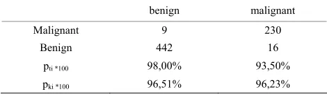
Table 17 shows the performance of the Matlab knn. ProtoClass does not clearly outperform Matlab knn on this dataset. Table 18 shows the performance of Naïve Bayes Classifier. The performance is only for the class “benign” with the high number of samples better than the one of ProtoClass.
Overall the results from the three datasets summarised in this section demonstrate that measuring performance by using the overall accuracy of a classifier is inaccurate and insufficient when there is an unequal distribution of samples over classes, especially when one or more clas- ses are significantly under-represented. In addition, when the classifier uses the overall accuracy as feedback for feature subset selection, feature weighting and prototype selection are flawed as this approach encourages the classifier to ignore classes with a small number of mem-bers. Examining the contingency table and calculating the class specific quality measurements provides a more complete picture of classifier performance .
6. Discussion
We have studied the performance of some well-known classifiers such as Naïve Bayesian, decision tree induc-tion and k-NN classifiers with respect to our case-based classifier ProtoClass. This study was done on datasets where some classes are heavily under-represented. This is a characteristic of many medical applications.
classified. This results in a classifier that is heavily gen-eralized to over-represented classes and does not recog-nize the under-represented classes. For example, in the E. coli dataset (described in Section 4) there are two classes with only two cases. When the k-value is greater than 3, these cases will never be correctly classified since the over-represented classes will occupy the greater number of nearest cases. This observation is also true for Deci-sion Trees and Naïve Bayesian classifiers. To judge the true performance of a classifier we need to have more detailed observations about the output of the classifier. Such detailed observations are provided by the contin-gency table in Section 3 that allow us to derive more specific accuracy measures. We choose the class-specific classification quality described in Section 3.
The prototype selection algorithm used here is prob-lematic with respect to the evaluation approach. Relying on the overall accuracy of the design dataset to assess whether two cases should be merged to form a new pro-totype tends to encourage over-generalization where un-der-represented classes are neglected in favor of changes to well-populated classes that have a greater impact on the accuracy of the classifier. Generalization based on the accuracy seems to be flawed and reduces the effective-ness of case-based classifiers in handling datasets with under-represented classes. We are currently investigating alternative methods to improve generalization in case-ba- sed classifiers that would also take into account under- represented classes in spite of the well-represented classes.
The question is what is important from the point of view of methodology? FS is the least computationally expensive method because it is implemented using the best first search strategy. FW is more expensive then FS but less expensive than PS. FS and FW fall into the same group of methods. That means FS changes the weights of a feature from “1” (feature present) to “0” (feature turned off). It can be seen as a feature weighting approach. When FS does not bring about any improvement, FW is less likely to provide worthwhile benefits. With respect to methodology, this observation indicates that it might be beneficial to not conduct feature weighting if feature subset selection shows no improvement. This rule-of- thumb would greatly reduce the required computational time.
PS is the most computationally expensive method. In case of the data sets from the machine learning repository this method did not have much impact since the data sets have been heavily pre-cleaned over the years. For a real world data set, where redundant samples, duplicates and variations among the samples are common, this method has a more significant impact [6].
7. Future Work and Conclusions
The work described in this paper is a further
develop-ment of our case-based classification work [6]. We have introduced new evaluation measures into the design of such a classifier and have more deeply studied the be-havior of the options of the classifier according to the different accuracy measures.
The study in [6] relied on an expert-selected real-wor- ld image dataset that was considered by the expert as providing prototypical images for this application. The central focus of this study was the conceptual proof of such an approach for image classification as well as the evaluation of the usefulness of the expert-selected proto-types. The study was based on more specific evalu- ation measures for such a classifier and focused on a methodology for handling the different options of such a classifier.
Rather than relying on the overall accuracy to properly assess the performance of the classifier, we create the contingency table and calculate more specific accuracy measures from it. Even for datasets with a small number of samples in a class, the k-NN classifier is not the best choice since this classifier also tends to prefer well-repre- sented classes. Further work will evaluate the impact of feature weighting and changing the similarity measure. Generalization methods for datasets with well-represent- ed classes despite the presence of under-represented clas- ses will be further studied. This will result in a more det- ailed methodology for applying our case-based classifier.
REFERENCES
[1] A. Asuncion and D. J. Newman. “UCI machine learning repository,”[http://www.ics.uci.edu/~mlearn/MLReposit- ory.html] University of California, School of Informa- tion and Computer Science, Irvine, CA, 2007.
[2] C. L. Chang, “Finding prototypes for nearest neighbor classifiers,” IEEE Transactions on Computers, Vol. C-23, No. 11, pp. 1179–1184, 1974.
[3] P. Perner, “Data mining on multimedia data,” Springer Verlag, lncs 2558, 2002
[4] D. Wettschereck and D. W. Aha, “Weighting Features,” M. Veloso and A. Aamodt, in Case-Based Reasoning Research and Development, M. lncs 1010, Springer- Verlag, Berlin Heidelberg, pp. 347–358, 1995.
[5] D. W. Aha, D. Kibler, and M. K. Albert, “Instance-based learning algorithm,” Machine Learning, Vol. 6, No. 1, pp. 37–66, 1991.
[6] P. Perner, “Prototype-based classification,” Applied Intel-ligence, Vol. 28, pp. 238–246, 2008.
[7] P. Perner, U. Zscherpel, and C. Jacobsen, “A comparision between neural networks and decision trees based on data from industrial radiographic testing,” Pattern Recognition Letters, Vol. 22, pp. 47–54, 2001.
[9] I. H. Witten and E. Frank, Data Mining: Practical ma-chine learning tools and techniques, 2nd Edition, Morgan
Kaufmann, San Francisco, 2005.
[10] DECISION MASTER, http://www.ibai-solutions.de. [11] P. Horton and K. Nakai, “Better prediction of protein
cel-lular localization sites with the it k nearest neighbors clas-sifier” Proceeding of the International Conference on
Intel-ligent Systems in Molecular Biology, pp. 147–152 1997. [12] C. A. Ratanamahatana and D. Gunopulos. “Scaling up the