Information geometry and local asymptotic normality for multi parameter estimation of quantum Markov dynamics

Information geometry and local asymptotic normality for multi-parameter estimation of quantum Markov dynamics

Madalin Guta1,a) and Jukka Kiukas2,b)

1)_{School of Mathematical Sciences, University of Nottingham, University Park,}

Nottingham, NG7 2RD, UK

2)_{Department of Mathematics, Aberystwyth University, Penglais, Aberystwyth,}

Ceredigion, SY23 3BZ, UK

(Dated: 20 March 2017)

This paper deals with the problem of identifying and estimating dynamical parameters of continuous-time Markovian quantum open systems, in the input-output formalism. First, we characterise the space of identifiable parameters for ergodic dynamics, assuming full access to the output state for arbitrarily long times, and show that the equivalence classes of undistinguishable parameters are orbits of a Lie group acting on the space of dynamical parameters. Second, we define an information geometric structure on this space, including a principal bundle given by the action of the group, as well as a com-patible connection, and a Riemannian metric based on the quantum Fisher information of the output. We compute the metric explicitly in terms of the Markov covariance of certain ”fluctuation operators”, and relate it to the horizontal bundle of the connec-tion. Third, we show that the system-output and reduced output state satisfy local asymptotic normality, i.e. they can be approximated by a Gaussian model consisting of coherent states of a multimode continuos variables system constructed from the Markov covariance “data”. We illustrate the result by working out the details of the information geometry of a physically relevant two-level system.

I. INTRODUCTION

The input-output formalism12,23 _{is fundamental to key areas of quantum open systems}

the-ory such as Markov dynamics, continuous-time measurements and filtering thethe-ory7,10, quantum networks25 _{and feedback control}8,39_{. The formalism serves as a platform which integrates in}

a common language methods from control engineering, classical and quantum stochastic pro-cesses, non-equilibrium statistical mechanics, and quantum information. In this paper we aim to further expand this platform by adopting a system identification42 _{perspective. Concretely,}

we investigate which dynamical parameters of an open system can be estimated from the out-put state (identifiability problem), how the associated quantum Fisher information arises from the structure of the parameter manifold (information geometry), and how the multi-parameter statistical model defined by the output state can be approximated by a quantum Gaussian model (local asymptotic normality).

System

Input _Output

A1(t) Aout

1 (t)

Aout

k (t)

Ak(t) N(t)

B(t) H, L1_{, . . . , L}k

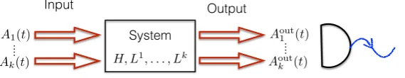
FIG. 1. Continuous-time Markovian dynamics of an open quantum system in the input-output for-malism. Input fields Ai(t) interact with the system, so that the joint unitary transformation UD(t)

depends on the dynamical parameter D:= (H, L1_{, . . . , L}k_{) where H is the system Hamiltonian and}

Li _{are the coupling (jump) operators with the input fields. The output state carry information about}

D, which can be estimated by measuring the output fields.

In a typical quantum input-output set-up, an open system (e.g. an atom, or a cavity mode) is driven by an input consisting of the vacuum or coherent state of the electromagnetic field, the latter being modelled by a continuum of Bosonic modes representing the incoming “quantum noise”, see Figure 1. The input interacts with the system in a Markovian fashion, with joint unitary evolutionUD(t) determined by the “dynamical parameters”D:= (H, L1, . . . , Lk), where H is the system Hamiltonian and Li is the coupling operator to thei-th input mode.

The output fields carry information about the dynamical parameterD, and can be monitored by means of continuous-time measurements, or may be “post-processed”, e.g. by using feed-forward or feedback schemes53_{. However, since such schemes often rely on the knowledge of the}

dynamics, it is important to develop efficient methods for estimating the unknown parameters entering the dynamics. Our goal here is not to propose or analyse specific measurement and estimation schemes (see e.g.14,20,21,43 _{for related results), but rather investigate the statistical}

We envisage that the structure of the output state uncovered here will be relevant not only for designing efficient measurement schemes (cf.28 _{for optimal estimation of qubit states) but also}

for applications in quantum metrology44 _{and quantum control, including feedback.}

In our analysis we assume that the system is finite dimensional, and the input is stationary (time independent). We also assume that the dynamics is ergodic, i.e. the system has a unique strictly positive stationary state ρD_ss, in which case any initial state converges to ρD_ss and the output becomes stationary in time. From a quantum information perspective, the system-output state _|Ψs+o_D (t)_i associated to the time interval [0, t] is a continuous matrix product state52, and the output state ρout_D (t) is a continuous version of a purely generated finitely correlated state18_{. Our results are therefore relevant for the problem of estimating such states,}

whose discrete version was considered in6 _{from the perspective of quantum tomography of spin}

chains.

Since we deal with a multi-parameter statistical problem, we adopt a differential geometry viewpoint in the spirit of the theory of information geometry2. This allows us to characterise the manifold of identifiable parameters as the quotient of the parameter space with respect to a group of transformations leaving the output state invariant (see Theorem 1), thus extending our previous results for discrete time quantum Markov chains31. An analogous differential geometric construction has been presented in33,34 _{for parametrisations of discrete matrix product states,}

and a related approach has been used in studying the manifold of correlation matrices for stationary states of certain specific open quantum systems4.

Furthermore, we show that the quantum Fisher information (QFI)11,36_{of the output is closely}

related to the covariance of certain “fluctuation operators”, which we study in detail in section V. The covariance defines a Riemannian metric on the space of identifiable parameters, and provides a complex structure and a positive inner product on the tangent space of identifiable parameters. An alternative approach to computing the quantum Fisher information is described in22_{, see also}44 _and16_.

With the help of this differential geometric structure we construct an associated algebra of canonical commutation relations (CCR), and a family of coherent states whose QFI is equal to the QFI per time unit of the output state. The latter will play the role of limit Gaussian model below.

Local asymptotic normality (LAN) is a key concept in asymptotic statistics, that describes how certain statistical models can be approximated by simpler Gaussian models, with vanishing error in the limit of large “sample size”. This phenomenon occurs for instance in the case of models consisting of independent, identically distributed samples41_{, but also for multiple}

the general theory of convergence of models was discussed in24,29, and LAN for ensembles of independent finite dimensional systems was established in40_{. For quantum Markov dynamics,}

LAN for one-dimensional parameter models was discussed in27,31 _{for discrete time, and in}13 _for

continuous-time. Here we extend the latter to the multi-dimensional model where all identi-fiable parameters are assumed to be unknown; this brings forward the information-geometric aspects, which do not play a significant role in a one-parameter setting. Theorem 2 shows that the system-output state and (reduced) output state models converge to the Gaussian model consisting of a family of coherent states of the above mentioned CCR algebra, in the limit of large times.

The present investigation suggests several interesting future lines of research. One direction is to understand the physical significance of the geodesic distance of the Fisher metric and the relation to quantum speed limit51 and thermodynamic metrics50. Another direction is to show that fluctuation operators satisfy the Central Limit Theorem, and identify the measurement which achieves the optimal estimation precision. Building on32, one can develop a similar theory for the identification of quantum linear input-output systems in the stationary regime, i.e. from the “power spectrum”. Moreover, the extension of the current theory to non-ergodic dynamics and the analysis of “metastable”45 or “near phase transition”44systems is important due to its relevance for quantum metrology. Finally, our framework has a number of interesting generali-sations connected with other ongoing mathematical work on quantum stochastic evolutions. In particular, when the stationary state manifold is nontrivial (non-ergodic case), one can discuss conserved quantities and adiabatic transport1,3,26_{. From the more technical point of view, our}

manifold of dynamical parameters actually has a natural Lie group structure17; reformulation of our results in this more structured framework could be useful especially for applications to control theory.

In order to increase the accessibility of the paper, we collect the main constructions and results in the next section.

II. OVERVIEW OF RESULTS

stochastic differential equation

dUD(t) =

k X

i=1

(iH_⊗1Fdt+Li⊗dA∗_i(t)−Li∗⊗dAi(t))−

1 2

k X

i=1

Li∗Li_⊗1Fdt

!

UD(t).

Above, dAi(t) anddA∗i(t) are the time increments of input annihilation and creation operators

of k Bosonic input channels, acting on the Fock space _F over L2₍

R+)⊗Ck. The reduced

system evolution is governed by an ergodic Markov semigroup with Lindblad generator _WD, and unique stationary state ρD_ss. The output state after time t is obtained by tracing out the system, ρout_D (t) = trs(|Ψ_Ds+o(t)ihΨs+o_D (t)|). For long times the system converges to the stationary

state, and the output becomes stationary in time.

D

gD P _Derg

Identifiable parameters Equivalence classes

Tnonid

D

Tid

D

˙ Da

˙ Db

D

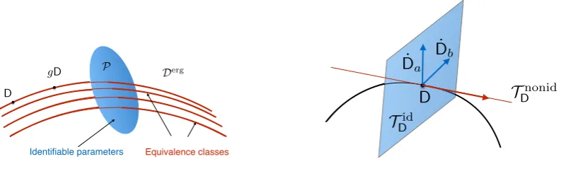
FIG. 2. Left panel: the space of ergodic dynamical parameters Derg _{as principle G-bundle over the} base manifold _P of identifiable parameters. Equivalence classes (red lines) of dynamical parameters

with identical outputs. Right panel: the tangent space at the pointDdecomposes as direct sum of the tangent space _Tnonid

D to the orbit of the group action, and the space TDid of “identifiable directions”

defined by the identity E0

D( ˙D) = 0. The Markov covariance defines a complex structure and an inner

product on_Tid

D , such that the QFI rate isfa,b= 4Re( ˙Da,D˙a)D.

Section IV discusses the identifiability problem in the stationary setting, see Figure 2. We define an equivalence relation between dynamical parameters for which the stationary output states are identical for all timest. In Theorem 1 we show that two dynamical parametersDand D0 are equivalentif and only if they are related by the “gauge transformation”H0 =W∗HW+ r1 andL0_i =W∗LiW, whereW is unitary andris a real constant. From a differential geometry

viewpoint, the space of identifiable parameters is the quotient _P :=_Derg_{/G, whereD}erg _{is the}

manifold of dynamical parametersDwith ergodic dynamics, andG=P U(d)_×Ris the group of “gauge transformations” whose orbits are the equivalence classes of parameters. In particular, we show that _Derg _{is a principalG-bundle over the base manifold P. The vertical bundle over}

Derg _{consists of subspacesT}nonid

“non-indentifiable” components (i.e. _TD =TDnonid⊕ TDid), such a decomposition can be obtained from a principal connection, in a covariant way. A natural choice of connection is provided by the information geometry, as discussed below. This approach to system identification often appears in the classical setting, and the advantage is that one gains insight in the geometric structure of the parameter manifold, beyond the direct computation of the Fisher information. For instance, the connection can be useful for developing recursive estimation algorithms based on geodesics of the manifold35. For the standard theory of connections on principal bundles, see e.g.38.

In Section V we derive the information geometric structure of the statistical estimation problem at hand. Before discussing the statistical aspects, we describe the basic elements of a theory of “output fluctuations” which is essential for information geometry, but has an interest in its own and deserves to be further investigated. For each (k+ 1)-tuple of system operators

X= (X0, X1, . . . , Xk)_∈M(_Cd)k+1 we define the associated fluctuation operator _FD,t(X) given

by the quantum stochastic integral

FD,t(X) =

1 √ t

Z t

0

i

k X

i=1

jD,s(Xi)dA∗i(s) +jD,s ◦ CD(X0)ds

!

, _CD(X) := X−tr[ρDssX]1,

where jD,s(X) := U_D∗(s)XUD(s) is the time-evolved operator X. The covariance of FD,t(X)

converges in the limit of large times, and defines a positive (but degenerate) inner product on M(_Cd₎k+1 _{(cf. Proposition 1 for the explicit formula)}

(X,Y)D = lim

t→∞hFD,t(X) ∗

FD,t(Y)i.

Furthermore, in Propositions 1 and 2 we construct a linear map RD :M(Cd)k+1 →M(Cd)k+1

such that RD is a projection onto the subspace of operators of the form (0, Y1, . . . , Yk) ∈ M(_Cd₎k+1_{, and the kernel of R}

D is the subspace of degenerate vectors of the inner product. With this definition, the inner product take the following simple form

(X,Y)D =

k X

i=1

trρD_ssRD(X)i∗RD(Y)i

.

We denote by ˙D= ( ˙H,L˙1, . . . ,L˙k) an element of the tangent space_TD. Thereal linear mapXD defined below plays an important role in connecting fluctuation operators with the information geometry:

XD :TD →M(Cd)k+1

˙

D_7→(_ED( ˙D),L˙1, . . . ,L˙k) where _ED is the map

ED :TD →M(Cd)

ED : ˙D7→H˙ + Im

k X

i=1

Here the second term in _ED is due to quantum Ito calculus, hence in some sense represents the effects of the stochastic output on the information geometry. Using the map XD we define a real inner product on the tangent space _TD

( ˙D,D˙0)_7−→Re(XD( ˙D),XD( ˙D0))D.

Moreover, sinceXD is injective, we can use it to define a projection PD =XD−1◦RD◦XD acting on _TD. Its kernel is the vertical space TDnonid whose vectors correspond to infinitesimal “gauge transformations”, and are the degenerate vectors of the inner product. The range ofPD consists of tangent vectors satisfying the condition _ED( ˙D) = 0. In particular, since PD is a projection, the tangent space can be decomposed into “identifiable” and “non-identifiable” directions (see right panel of Figure 2)

TD = ranPD⊕kerPD =TDid⊕ TDnonid

whose statistical interpretation is discussed below. This split has also an interesting differen-tial geometric interpretation: the above tangent space decomposition, and inner product are covariant with respect to the action of the group G and define a connection on the resulting principal G-bundle, with the associated Lie algebra valued one-form

ωD :TD →g, ωD( ˙D) = (−iWD−1◦ CD◦ ED( ˙D),tr[ρDssED( ˙D)])

explicitly depending on the map_ED( ˙D) containing the essential quantum Ito correction. More-over, the strictly positive inner product on_TDid induces a strictly positive inner product on the tangent space_T[D]to the point [D] in the base spaceP =Derg/Gof identifiable parameters. As

we will see below, this Riemannian metric is closely connected to the quantum Fisher infor-mation rate of the output state, so we will refer to it as the information geometry of the open quantum system, in analogy to the classical case2_.

Let us consider now the problem of estimating the dynamical parameter D. Although the key constructions could be introduced in a “coordinate free” way, in order to emphasise the statistical aspects we choose to work with a given (but arbitrary) parametrisation θ _7→ Dθ

of _Derg, where θ is an unknown parameter belonging to an open subset of _Rm, with m := dim(_Derg_{). At a given point D = D}

θ ∈ Derg, we define the tangent vectors ˙Da := ∂D/∂θa =

( ˙Ha,L˙1a, . . . ,L˙ka) describing infinitesimal changes of the coordinate θa, for a = 1, . . . , m; these

vectors form a basis of the tangent space _TD.

We consider now the m_×m quantum Fisher information (QFI) matrix Fθ_{(t) associated to}

the system-output state _|Ψs+o_D

θ (t)i. The QFI is proportional to the real part of the covariance matrix of (centred) “generators” G0

θ,a(t) of infinitesimal changes with respect to parameter

componentθa11. We show that the generatorG0θ,a(t) (normalised byt

afluctuation operator _Ft(XD( ˙Da)), using the mapXD defined above. As consequence, the QFI grows linearly in time, and the QFI rate per time unit fθ = limt→∞Fθ(t)/t can be expressed

in terms of the Markov covariance as

f_a,bθ = 4Re(XD( ˙Da),XD( ˙Db))D = 4Re(RDXD( ˙Da), RDXD( ˙Db))D = 4

k X

i=1

Re trhρD_ssL˙i_a−i[Li,_W−_D1_{◦ ED}0( ˙Da)]

∗

˙

L_bi ₋i[Li,_WD−1_{◦ ED}0( ˙Db)] i

.

where_WD is the Lindblad operator atDandED0 =CD◦ED. In particular, the Fisher information rate associated to directions in vertical bundle _Tnonid

D (gauge transformations) is equal to zero as expected from the invariance of the output state. This follows from the fact that XD maps Tnonid

D into kerRD.

Above we saw that the real part of the Markov covariance (_·,_·)D defines a positive defi-nite inner product on the real space _TDid. In fact, _TDid can be made into a complex space by introducing the complex structure

JD :TDid → TDid

JD : ( ˙H,L˙1, . . . ,L˙k)7→

k X

i=1

Re ˙Li∗Li, iL˙1, . . . , iL˙k

!

. (1)

With this definition the mapXD becomes an isomorphism of complex spaces and (·,·)D defines a complex inner product on (_Tid

D ,JD). Using the imaginary part σD of the inner product, we

define the canonical commutation relations (CCR) algebra CCR(_TDid, σD) generated by Weyl operators with commutation relations

W( ˙D)W( ˙D0) = eiσD( ˙D,D˙0)W( ˙D+ ˙D0), W(₋D˙) =W( ˙D)∗, D,˙ D˙0 _{∈ TD}id.

Following a standard construction we define the Fock representation and the coherent states |D˙_i:=W( ˙D)_|0_i, where _|0_iis the vacuum state_h0_|W( ˙D)_|0_i= exp(₋( ˙D,D˙)D/2) This model will be interpreted below as limit of the output state model for large times.

Section VI details the above constructions in the case of special one dimensional models, and for a general multidimensional model for a two dimensional system.

In section VII we study the asymptotic statistical structure of the output state. The main result is the local asymptotic normality (LAN) Theorem 2 which shows that both the system-output state, and the stationary system-output state can be approximated by coherent states of the CCR algebraCCR(_Tid

D , σD). Below we give a brief description of the result and its interpreta-tion.

Let us consider a parametrisation u_7→ [D]u of (an open subset of) the space of identifiable

u v

s+o v/pt(t)

E

s+o u/pt(t)

E

System-output states at time t Limit Gaussian shift model

t! 1

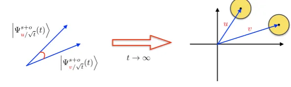
FIG. 3. Local asymptotic normality as weak convergence to the Gaussian limit. The inner products

of system-output states with local parameter u, v converge (uniformly) to the inner products of the corresponding coherent state_|u_i and _|v_i, in the limit of large times.

[D0] = [D]u=0. We define the time-indexed family of “local” statistical models

˜ Qt:=

n

ρout_u/√

t(t) :u∈ O ⊂R

dim(P)o

which consist of the output state for unknown parameter valuesu/√t in a shrinking ball of size scaling as the statistical uncertainty. The local model ˜_Qt captures the asymptotic properties

of the quantum output state for parameters in a neighbourhood of [D0], and it can be justified

operationally by means of adaptive procedures whereby a “small part” of the output can be used to localise the parameter, while the “remaining part” can be used for estimating the local parameter u (cf.30 _{for a similar argument in the state estimation setup).}

To define the system-output statistical model let us consider a horisontal section s : _{P →} Derg _{of the principal bundle, i.e. the tangent space to s(P) at D is the horisontal space T}id

D . Let

Qt:=nΨs+o_u/√_t(t) E

:u_{∈ O ⊂R}dim(P)o,

be the quantum statistical model where

Ψs+o

u/√t(t) E

is the joint system-output state at time t at the dynamical parameter Du = s([D]u). The reasons for using a horisontal section in

defining the model are as follows. While the stationary output state depends only on the identifiable parameters in _P, the system-output state is also sensitive to the location of the parameter within an orbit. It turns out that the asymptotic properties can be captured most transparently by choosing a horisontal section which sets certain unphysical phase factors to zero and allows us to understand the model directly in terms of the geometric properties of the vector state, as explained below.

Finally, we define the Gaussian model

G :=ρu :=|uihu|:u∈ O ⊂Rdim(P)

where _|u_i = W(P_auaD˙a)|0i is the coherent state of the CCR algebra CCR(TDid0, σ

D0_{). By}

which also is the QFI of the output state with respect to the local parameter u, rather than the “true” parameter u/√t.

The first version of LAN states that _Qt converges (weakly) to G for large times in the sense

of convergence of the inner products (uniformly in u, v _{∈ O}), as illustrated in Figure 3

lim

n→∞

D

Ψs+o_u/√

t(t) Ψs+o_v/√

t(t) E

=_hu_|v_i.

Since pure state models are fully characterised by the inner products, the convergence simply means that for large times the geometry of the system-output states is very similar to that of the coherent states. Although intuitive, this notion of convergence is not suitable for mixed states such as that of the output, and does not have a direct operational meaning. In the second version of LAN we show that the output models ˜_Qt converge strongly toG in the sense

that there exist channels Tt and St such that

lim

t→∞sup_u∈O

Tt

ρout_u/√

t(t)

−ρu

1

= 0

lim

t→∞sup_u∈O

St(ρu)−ρout_u/√_t(t)

1

= 0.

A concrete consequence of this “convergence to Gaussianity” is that the QFI computed above is asymptotically “achievable” in the sense that the estimation of dynamical parameters reduces to that of estimating a Gaussian displacement family with QFI equal tofa,b. Similarly to LAN

for ensembles of identical states30_{, the result implies that the optimal measurement is a linear}

one (i.e. of homodyne and heterodyne type) and the errors are normally distributed. However, since this paper concentrates on the structure of the quantum states, the measurement and estimation procedures are not discussed here.

III. PRELIMINARIES ON QUANTUM MARKOV PROCESSES

We begin by introducing notations and necessary background about the input-output for-malism of continuous-time quantum Markov processes23_{. The formalism describes the joint}

unitary evolution of an open quantum system interacting with a Bosonic environment in the Markov regime, cf. Figure 1. From this, one can derive the reduced (master) dynamics of the system, as well as the stochastic Schr¨odinger equations for quantum trajectories, describing the stochastic evolution of the system conditional on observations produced by a continuous-time measurement on the environment. However, in this paper we will be mainly interested in the output quantum state, i.e. the state of the environment after the interaction with the system.

Throughout the paper we assume the system to be finite-dimensional, with Hilbert space H = _Cd_{, and associated algebra of observables A = M(}

dynamics is specified by thesystem Hamiltonian H, together with thequantum jump operators L1_{, . . . , L}k_{. We denote these collectively by}

D= (H, L1, . . . , Lk) = (H,L)_{∈ D}:=Msa(Cd)×M(Cd)k,

and refer to each D_{∈ D} as adynamical parameter, and to _D as manifold (space) of dynamical parameters.

A. Environment as quantum noise.

In the Markov approximation, the interaction can be described as the unitary scattering of incoming vacuum Bosonic fields, caused by the continuous interaction with the system. The environment is modelled by k Bosonic channels whose Hilbert space is the Fock space

F :=_F(hk) = C|Ωi ⊕

∞

M

l=1 h⊗sl

k

where hk := L2(R+)⊗Ck is the one particle space of the k channels, and |Ωi is the vacuum

vector. Similarly, we denote by _F(a,b) the Fock space over L2((a, b)) ⊗Ck. For each time

t, the symmetric Fock space decomposes as tensor product _F = _F(0,t)⊗ F(t,∞) between the

space of excitations up to time t (the past) and after time t (the future). The fundamental environment degrees of freedom are the annihilation and creation operators of the ith channel Ai(f) :=A(|fi ⊗ |ii) and respectively A∗i(g) := Ai(g)∗, which are defined in a standard way46

for all _|f_i,_|g_{i ∈}L2₍

R+), and satisfy the commutation relations

[A∗_i(g), Aj(f)] = Imhf|giδi,j1.

In particular, we will deal with the annihilation and creation processes Ai(t) := Ai(χ[0,t]) and

A∗_i(t), where t _{∈ R}+ represents time23,46. These processes are the quantum analogue of the

“classical” Wiener process and can be used to define quantum stochastic integrals of the form

I(t) =

Z t

0

k X

i=1

Mi(s)dAi(s) +Ni(s)dA∗i(s)

+P(s)ds

whereMi_{(s), N}i_{(s), P(s) aretime-adapted operator valued integrands, i.e. they are of the form}

X(s)_⊗1[s,∞) with respect to the decompositionF =F(0,s)⊗ F(s,∞). Quantum stochastic

inte-grals can be formally multiplied, and the productI1(t)I2(t) of two such integrals is a stochastic

integral whose increment is given by

d(I1(t)I2(t)) = dI1(t)·I2(t) +I1(t)·dI2(t) +dI1(t)·dI2(t) (2)

where the third terms is theIto correction which can computed by using the quantum Ito rule

dAi(t)dA∗j(t) = δi,jdt (3)

B. Interaction as input-output scattering.

We now introduce the coupling between system and the Bosonic environment, and the corresponding unitary evolution. Each dynamical parameter D = (H,L) determines a unique continuous family UD(t) of unitary operators (cocycles) describing evolution of the system and environment in the interaction picture with respect to the free evolution of the fields, the latter being given by the second quantisation of the right shift on L2(_R). The unitaries are defined as the solution of the quantum stochastic differential equation (QSDE)

dUD(t) =

k X

i=1

(Li_⊗dA∗_i(t)₋Li∗_⊗dAi(t))−iHeff ⊗1Fdt

!

UD(t), (4)

with initial condition UD(0) = 1. Here, Heff is the effective Hamiltonian Heff := H −

i

2

Pk i=1Li

∗_Li _{which generates a semigroup S}

D(t) = e−itHeff of contractions on the system’s space, and describes the evolution of the system between consecutive quantum jumps. The imaginary part ₂i Pk_i=1Li∗Li is the Ito correction which insures that UD(t) is unitary. For sim-plicity of notation, from now on we will omit the tensor product and simply write Li_⊗dA∗

i(t)

as LidA∗_i(t), an similarly for other integrands.

If the system is initialised in state _|ϕ_i and the input fields are in the vacuum state_|Ω_i, then the state of the system together with the output after time t is given by

|Ψs+o_D (t)_i=UD(t)|ϕ⊗Ωi=VD(t)|ϕi, (5)

where VD(t) :H → H ⊗ F is a family of isometries defined by the second equality. Theoutput state is the state of the scattered field modes after the interaction with the system, and is obtained by tracing out the system

ρout_D (t) = trH[|Ψs+o_D (t)ihΨs+o(t)|].

Let us denote by jD,t(X) :=UD(t)∗(X⊗1F)UD(t) the Heisenberg evolved system operator X. Using equation (4), we find that the operators satisfy the quantum Langevin equation

djD,t(X) = X

i

jD,t([X, Li])dA∗i(t) +jD,t([Li∗, X])dAi(t)

+jD,t(WD(X))dt. (6)

where

WD(·) =−i(·)Heff +iHeff∗ (·) +

k X

i=1

Li∗(_·)Li

is called the Lindblad generator. Its significance can understood by considering the reduced Heisenberg evolution of the system TD,t : A → A defined by taking the expectation over the

environment

From (6) we find dTD,t(X) = dhΩ|jD,t(X)|Ωi= WD(TD,t(X)) which means that TD,t is a trace

preserving completely positive semigroup with generator _WD. The generator is said to be ergodic, if it has a unique stationary state ρD_ss (i.e. [_WD]∗(ρD_ss) = 0) which has full rank. In this

case19

lim

t→∞TD,t = limt→∞

1 t

Z t

0

TD,sds= tr[ρDss(·)]1. (8)

Since we are interested in the long-time asymptotic properties of the output state, we assume that the dynamics has reached stationarity, or equivalently that the initial state of the system is ρD_ss. In this case the output state is time-stationary and is given by

ρout_D (t) = trH[UD(t)(ρDss⊗ |ΩihΩ|)UD(t)

∗

]. (9)

Since ρD_ss is a stationary state, the range of _WD is included in

BD

0 ={X |tr[ρDssX] = 0}.

By ergodicity,1 is the only fixed point ofetWD_{, and hence ker(}

WD) is spanned by 1∈ B/ D0. This

implies that the range has dimension d2_{−1 = dimB}D

0, i.e. WD is surjective onto BD0, and the

restriction of_WDontoB0Dis injective. HenceWDis invertible onBD0, and we letW −1

D :B0D → B0D

denote the inverse. Furthermore, the following limit exists:

−W−D1 = lim_t→∞

Z t

0

TD,sds. (10)

IV. IDENTIFIABILITY OF CONTINUOUS QUANTUM MARKOV

PROCESSES

This section deals with the problem of characterising the equivalence classes of Markov dynamics with identical stationary output states. We restrict ourselves to ergodic Markov processes, although similar results are expected to hold more generally. Similar results have been obtained in31 _{fordiscrete time quantum Markov processes.}

Let _Derg denote the open submanifold of _D consisting of dynamical parameters for which the associated Markov process is ergodic; this will be the relevant parameter set for subsequent considerations. Note that _Derg _{is indeed an open subset of D since ergodicity (i.e. non-zero}

spectral gap and full rank stationary state) is preserved under small perturbations.

Of course, the same equivalence can be formulated for arbitrary parameters in _D. However, it turns out that when restricted to_Derg_{, the equivalence classes have a simple characterisation}

in terms of the following transformations:

(PM) Phase conjugation on the Hamiltonian:

(H, L1, . . . , Lk)_7→(H+r1, L1, . . . , Lk), (r_∈R).

(UC) Conjugation by system unitary W:

(H, L1, . . . , Lk)_7→(W∗HW, W∗L1W, . . . , W∗LkW).

Indeed, it is easy to verify that (PM) and (UC) do not change the output of the associated continuous Markov process. The following Theorem shows that the converse is also true. The details of the proof can be found in Appendix VIII.

Theorem 1. Let D,D0 _{∈ D}erg_{. Then Dand D}0 _{are output-equivalent if and only if they can be}

obtained from each other via the transformations (UC) and (PM).

The interpretation of the result is that parameters along the equivalence classes described by the transformations (UC) and (PM) are not identifiable, while the identifiable parameters are “transversal” to these classes, as illustrated in Figure 2. It is now convenient to formulate the equivalence classes in terms of an action of the appropriate Lie group G:=P U(d)_×R. On Derg _{we use transformations (PM) and (UC) to set up the action:}

G_{× D}erg _{→ D}erg

(g,D)_7→gD:= (W∗HW, W∗L1W, . . . , W∗LkW) +a(1,0, . . . ,0), (11) g = (W, a)_∈P U(d)_×R, D= (H, L1, . . . , Lk)_{∈ D}erg.

Here P U(d) = U(d)/U(1) is the projective unitary group, equipped with its unique Lie group structure, and the above action is defined as the natural lift of the corresponding one forU(d). The reason to useP U(d) instead of U(d) will become clear from the proof of the Lemma below. The above theorem implies that the equivalence class [D]_{∈ P} is the orbit of D_{∈ D}erg under the action ofG, such that _P can be identified with the quotient _Derg_{/G. The following lemma}

which relies on the ergodicity assumption, is essential for understanding the structure of the quotient, as we will see below. In order to avoid confusion with the output equivalence, we identify W _∈P U(d) with a representative unitary operator without explicit indication.

Proof. The action defined via (11) is clearly smooth with respect to W, and a, hence its lift to the quotient Lie group P U(d)_×R is smooth as well. Since the group P U(d) is compact, and the rest is just a translation, it follows from elementary arguments that the smooth map G_{× D}erg _{→ D}erg_{× D}erg given by (g,D) _7→ (gD,D) is proper, i.e. preimage of every compact set is compact. This means that the action is proper. In order to show that the action is free, we need to use ergodicity as follows: suppose that gD=g0D for some D, and g = (W, a), g0 = (W0, a0); then a direct computation similar to the one in the proof of Lemma 2 in Appendix shows that _WD(W∗W0) =i(a−a0)W∗W0. Since ergodicity requires

lim

τ→∞e

iτ(a−a0)_W∗

W0 = tr[W∗W0ρss]I,

we must have a = a0 and W∗W0 a multiple of the identity. But this exactly means that W equals W0 as an element of the projective unitary group; hence g = g0. This proves that the action is free.

The fact that the group action preserves the equivalence classes, that is gD _∈ [D] for all D _{∈ D}erg_{, can now be formulated in differential geometric terms. Indeed, using the standard}

theory of Lie group actions on manifolds, we conclude from the above Lemma that the space of output equivalence classes

P =_{[D] : D_{∈ D}erg_}=_Derg/G

admits a unique smooth structure such that the quotient map π:_Derg_{→ P}

π(D) = [D], for all D_{∈ D}erg,

is a submersion, and _Derg _{is a principalG-bundle over P}38_{. Here the equivalence classes [D] are}

considered as fibres of the fiber bundle over the base manifold _P, that is, the map π has the local triviality property: each [D]_{∈ P} has an open neighbourhood U such that there exists a diffeomorphism

φ :π−1(U)_→U _×G,

which is G-equivariant, i.e. φ(gD) = gφ(D) where Gacts onU _×G asg([D], g0) := ([D], g0g−1). The term principal G-bundle refers to the fact that the group action preserves the fibres.

We can now use this differential geometric framework to describe local changes of identifiable parameters, via the tangent bundle _T of the manifold _Derg. In particular, the non-identifiable parameter changes along the equivalence classes correspond to the vertical bundle over _Derg

with the fibres

Tnonid

where π∗|_D is the push-forward tangent map of the canonical projection π at point D, and TD is the full tangent space at that point.

The group action is reflected in two ways at the level of tangent spaces. On the one hand, given any fixedg _∈G, the push-forwardg∗ of the map D7→gDmaps the fibres into each other

as

g∗TDnonid =TgnonidD .

This push-forward is simply obtained by differentiating the parameters in the standard chart

g∗( ˙H,L˙1, . . . ,L˙k) = (W∗HW, W˙ ∗L˙1W, . . . , W∗L˙kW), g = (W, a).

On the other hand, for any fixed D, the push-forward of g _7→gD defines a Lie algebra isomor-phism

D∗ :g→ T_Dnonid, (12)

so that different fibres all have the same dimension, which is that of the Lie algebra g. We can now explicitly compute this action. First of all, the Lie algebra of G can be conveniently written as

g=_{(₋iK, r)_|K _∈Msa(Cd)/R1, r ∈R}={(−iK, r)|K ∈Msa(Cd), tr[ρssK] = 0, r∈R},

(13) where the choice of the sign as well as the last identification is for later convenience. In particular, the subspace of non-identifiable directions is in one-to-one correspondence with this linear space. From this we already find the number of non-identifiable directions:

dim_TDnonid =d2₋1 + 1 =d2.

We stress that this result is crucially based on ergodicity, which ensures that the action is free; this is required for the push-forward D∗ to be an isomorphism. Now D∗ acts on an element

X = (₋iK, r)_∈g as

D∗(X) =

d

dt(exp(t(−iK, r))D)|t=0 = d

dt (e

itK_He−itK_{, e}itK_L1_e−itK_{, . . . , e}itK_Lk_e−itK_{) +t r(1,0, . . . ,0)|} t=0

= (i[H, K], i[L1, K], . . . , i[Lk, K]) +r(1,0, . . . ,0). (14)

Having now characterised the vertical bundle_Tnonid_{of non-identifiable directions, an obvious}

question arises: is there a natural way to choose complementary subspaces for identifiable directions in each fibre? This means choosing subspaces_TDid such that

If the subspaces are chosen smoothly, i.e. so as to define a fibre bundle _Tidover_Derg, the result is called a horizontal bundle _Tid_{, and in case it respects the group action, that is}

g∗T_Did =TgidD, (15)

it defines an principal connection on the manifold _Derg.

There is a natural way of defining a principal connection via its associated connection one-form; since this approach turns out to be relevant in our situation, we briefly explain the idea in the general level. As we have shown above, any ˙D_{∈ T}nonid

D can be generated by the action of the Lie algebra; ˙D = D∗(X) for some X ∈ g. Now suppose that we can associate to every

tangent vector ˙D _{∈ T}D an element ωD( ˙D) ∈ g which somehow describes the “part” of the parameter that results from the non-identifiable group action. Such a map should define a one-form ωD :T → gsatisfying the compatibility condition (sometimes called nondegeneracy)

˙

D=D∗(ωD( ˙D)), D˙ ∈ TDnonid, (16)

and theG-covariance condition

g∗ω= Ad_g−1 ◦ω, (17)

where g∗ is the pull-back of the action by g on the cotangent bundle, which simply acts as g∗ω( ˙D) = ωgD(g∗D˙) = ωgD(W∗DW˙ ) for g = (W, a), and the adjoint action is given by Adg−1(X) = (W∗XW, r+a).

Given such a map, we can then define the ”back-action”D∗◦ωD on the tangent space; due to the above compatibility condition, the back-action is a special projection of the tangent space onto the subspace _Tnonid

D . Hence, we can use its complementary projection

PD := Id−D∗◦ωD

to define the above horizontal bundle and the associated principal connection via

Tid

D := ranPD.

Indeed, the condition (15) holds because of (17). The mapω is called theconnection one-form, and P is the horizontal projection.

V. INFORMATION GEOMETRY FOR DYNAMICAL PARAMETER

ESTIMATION FROM THE OUTPUT STATE

Our goal is to describe quantitatively the precision with which unknown dynamical param-eters can be estimated by making measurements on the output state. As noted above, we will restrict our attention to dynamical parameters Dwhich belong to the open subset _Derg _{of D of}

ergodic Markov dynamics. As we will consider this problem in the limit of large times, the rel-evant dynamical regime is the stationary one; moreover, the statistical properties of the output state can be understood locally, by focusing on a shrinking neighbourhood of the parameter manifold _Derg whose size is of the order of the statistical uncertainty13,31. This will lead to the concept of local asymptotic normality discussed in section VII. In this section however, we focus on the information geometry of the system identification problem, more precisely on the quantum Fisher information matrix of the output state and its asymptotic behaviour, and its relationship with the covariance of certain quanta stochastic integrals called “fluctuation operators”. We will start by introducing the latter in a general set-up and then show how the former fits in this theory.

Section V A derives the quantum Fisher information of the system-output state as covari-ance of certain “generators”; section V B analyses more general “fluctuation operators” and looks at their Markov covariance; section V C deals with the information geometry structure, and connects the previous constructions, in particular it provides an explicit expression of the quantum Fisher information; section V D constructs an algebra of canonical commutation re-lations (multimode continuous variables system) and a family of coherent states which will be relevant later on for the local asymptotic result.

A. Quantum Fisher information of a parametric model

We pass now to a statistical setting where the dynamical parameter D is considered to be unknown. The changes in Dare encoded in its (partial) derivatives ˙D= ( ˙H,L˙1_{, . . . ,L˙}k_{), which}

will be seen as vectors in the tangent space _TD to Derg at the point D. Since the dynamics is ergodic, the system converges to a unique stationary state ρD_ss for large times, and we will denote by _h·iss the expectation with respect to the state ρDss⊗ |ΩihΩ|. In this subsection we

consider a generic statistical model and analyse the quantum Fisher information (QFI) of the output state; we will show that the QFI grows linearly with time and the rate can be expressed in terms of the Markov covariance inner product introduced below. Let

be a smooth family of dynamics parametrised by an unknown parameterθ _∈Rm which may be thought to encode our prior knowledge about the dynamics. In this subsection we work with this parametrisation, and hence identify Dθ with θ for simplicity. Note that this could be a

complete parametrisation of _Derg. The directional derivatives of Dθ are defined as

˙ Dθ,a:=

∂H ∂θa ,∂L 1 ∂θa

, . . . ,∂L

k

∂θa

= ( ˙Hθ,a,L˙1θ,a, . . . ,L˙kθ,a)∈ TDθ.

Recall that the QFI of an arbitrary multiparameter (smooth) family of pure states _|ψθi with

θ _∈Rm_{, is them×m positive real matrix with elements}11

F_a,bθ = 4Re

∂ψθ ∂θa ∂ψθ ∂θb − ψθ ∂ψθ ∂θb ∂ψθ ∂θa ψθ

, 1_≤a, b_≤m.

We apply this formula to the output state _|Ψs+o_θ (t)_i := Uθ(t)|ϕ ⊗Ωi generated with a θ

-dependent dynamical parameter Dθ, cf. equation (9). By differentiating with respect to θa we

get

U_θ∗(t) ∂ ∂θa

Ψout_θ (t) =U_θ∗(t) ˙Uθ,a(t)|ϕ⊗Ωi, U˙θ,a(t) :=

∂Uθ(t)

∂θa

. (18)

We will now show that the generator ₋iGθ,a(t) := Uθ∗(t) ˙Uθ,a(t) can be written as a quantum

stochastic integral. From (4) we have

dU_θ∗(t) =U_θ∗(t) X

i

(₋Li_θdA∗_i(t) +L_θi∗dAi(t))−(−iHθ+

1 2

X

i

Li_θ∗Li_θ)dt

!

,

dU˙θ(t) = X

i

( ˙Li_θ,adA∗_i(t)₋L˙_θ,ai∗ dAi(t))−(iH˙θ,a+

1 2

X

i

( ˙Li_θ,a∗ Li_θ+Li_θ∗L˙i_θ))dt

!

Uθ(t)

+ X

i

(Li_θdA∗_i(t)₋L_θi∗dAi(t))−(iHθ+

1 2

X

i

Li_θ∗Li_θ)dt

!

˙ Uθ(t).

Therefore, by applying the Ito rule (3) we get

dU_θ∗(t)_·dU˙θ,a(t) = Uθ(t)∗ X

i

Li_θ∗L˙i_θ,aU(t) +Li_θU˙θ(t)

dt.

and using (2) we obtain an explicit differential expression for the generator

dGθ,a(t) = id(Uθ∗(t) ˙Uθ,a(t))

=iX

i

jθ,t( ˙Liθ,a)dA

∗

i(t)−jθ,t( ˙Lθ,ai∗ )dAi(t)

+jθ,t H˙θ,a+ Im X

i

˙ Li_θ,a∗ Li_θ

!

dt

=iX

i

jθ,t( ˙Liθ,a)dA

∗

i(t)−jθ,t( ˙Lθ,ai∗ )dAi(t)

+jθ,t

Eθ( ˙Dθ,a)

dt (19)

where _Eθ =EDθ is the real linear map ED :TD →Msa(C

d_{) given by}

ED( ˙D) := ˙H+ Im

k X

i=1

˙

Later on we will see that this map turns out to play a crucial role in the construction of the horizontal bundle for the identifiable parameters, and in the definition of the CCR algebra in section V D.

The QFI can be written in terms of the covariance matrix of the generators Gθ,b(t)

F_a,bθ (t) = 4Re _hϕ_⊗Ω_|G∗_θ,a(t)Gθ,b(t)|ϕ⊗Ωi − hϕ⊗Ω|G∗θ,a(t)|ϕ⊗Ωihϕ⊗Ω|Gθ,a(t)|ϕ⊗Ωi

.

where the second term stems from the fact thatGθ,b(t) have non-zero mean. The generators are

in fact not uniquely defined: since dAi(t) annihilates the vacuum state, arbitrary annihilation

integrals can be added, while terms proportional to the identity produce only unphysical com-plex phases which do not change the state. We will therefore define a modified (non-selfadjoint) generator which “centres”Gθ,b(t) for large times, and lacks annihilations terms so that it is

con-sistent with the definition of “fluctuation operators” introduced in the next subsection. The modified generator is given by the quantum stochastic integral with differential form

dG0_θ,a(t) = i

k X

i=1

jt( ˙Liθ,a)dA

∗

i(t) +

jθ,t(EDθ( ˙Dθ,a))−Tr

ρD_ssEDθ( ˙Dθ,a)

dt. (21)

By ergodicity, its rescaled mean converges to zero

lim

t→∞

1

thϕ⊗Ω|G

0

θ,a(t)|ϕ⊗Ωi= 0

For large times, the QFI matrix elements scale linearly with t and the leading contribution is given by the quantum Fisher information rate

f_a,bθ := lim

t→∞

F_a,bθ (t)

t = limt→∞

1

t4Rehϕ⊗Ω|G

0∗

θ,a(t)G0θ,b(t)|ϕ⊗Ωi. (22)

In the next section we prove the linear scaling and find an explicit expression of the QFI rate.

B. Fluctuation operators and the Markov covariance form

Our goal is now to formulate the QFI rate (22) in terms of certain quantum fluctuation operators, and subsequently compute it using quantum stochastic calculus. These fluctuation operators can be formulated in a slightly more general setting, which is naturally complex linear instead of real linear, and is also independent on the map_ED special to our setting. The dynamical parameter D will remain fixed throughout the section.

Recall that for any X _∈ M(_Cd) we let jD,t(X) denote the Heisenberg evolved system

observable defined by the Langevin equation (6). For an arbitrary (k + 1)-tuple X := (X0_{, X}1_{, . . . , X}k_{) ∈ M(}

quantum stochastic integral

FD,t(X) =

1 √ t

Z t

0

i

k X

i=1

jD,s(Xi)dA∗i(s) +jD,s◦ CD(X0)ds

!

, (23)

where the map

CD(X) := X−tr[ρDssX]1

“centers” the stationary mean of _FD,t(X) to zero:

hFD,t(X)iss =

1 √ t

Z t

0

tr[ρD_ssTD,s(X0−tr[ρDssX

0_{]1)]ds = √}1

t

Z t

0

tr[ρD_ss(X0₋tr[ρD_ssX0]1)]dt= 0.

The proof of the following crucial result is based on quantum Ito calculus, and can be found in the Appendix.

Proposition 1(Markov covariance for fluctuation operators). The following limit exists, is independent of the unit vector_|ϕ_{i ∈ H}, and defines a positive sesquilinear form (_·,_·)D on the complex linear space M(_Cd₎1+k _via

(X,Y)D := lim

t→∞hϕ⊗Ω|FD,t(X) ∗

FD,t(Y)|ϕ⊗Ωi= k X

i=1

trρD_ssRD(X)i∗RD(Y)i

,

where

RD(X) = (CD(X0), X1, . . . , Xk)− LD◦W−D1◦ CD(X

0_{), and}

LD(X) = WD(X), i[L1, X], . . . , i[Lk, X]

.

We call (_·,_·)D the Markov covariance inner product.

From this proposition it is clear that the map RD plays a central role; in particular, since ρD_ss has full rank, the kernel of the Markov covariance coincides with kerR_D. Also the range of RD turns out to be relevant. These subspaces can be characterised explicitly as follows.

Proposition 2. The operator RD is a projection, i.e. R2D =RD, with range and kernel

kerRD =

(_WD(K) +r1, i[L1, K], . . . , i[Lk, K])

K _∈M(_Cd), r_∈C ,

ranRD =

n

0, Y1, . . . , Yk Y1, . . . , Yk _∈M(_Cd)

o

.

Proof. First of all,X_∈kerRDif and only ifXi =i[Li,W−1(X0−tr[ρDssX0]1)] for alli= 1, . . . , k.

Since tr[ρD_ssWD(K)] = 0 for any K, the given form of the kernel follows. The range is clear from the definition, and the property R2

C. Markov covariance from a principal connection

We now proceed to show how the Markov covariance is naturally associated with a specific horizontal bundle for the principal G-bundle _Derg, and we also define a Riemannian metric on the manifold _Derg_{. In order to motivate this, we continue the the discussion from subsection}

V A. Indeed, the modified generator (21) can be expressed as a fluctuation operator

G0_θ,a(t) = √t_Ft(XD( ˙Dθ,a)),

where we have used the suggestive notation XD for the real linear isomorphism

XD :TD →Msa(Cd)×M(Cd)k (24)

˙

D= ( ˙H,L˙1, . . . ,L˙k)_7→(_ED( ˙D),L˙1, . . . ,L˙k), (25) where M(_Cd)k is now considered as a real linear space with dimension 2kd2, while Msa(Cd) is

naturally a real linear space. Therefore, using the explicit expression provided in Proposition 1, we obtain the following expression of the QFI rate (22) in the coordinates D =Dθ used in

subsection V A:

f_a,bθ = 4ReXD[ ˙Dθ,a], XD[ ˙Dθ,b]

D

= 4

k X

i=1

Re trhρD_ssL˙i_θ,a−i[Li_θ,_W−_D1_{◦ ED}0( ˙Dθa)]

∗

˙

L_θ,bi ₋i[Li_θ,_WD−1_{◦ ED}0( ˙Dθb)]

i

, (26)

where _E0

D =CD ◦ ED. The QFI rate inherits the positivity property of the Markov covariance, but also the fact that it may not be positive definite. In conclusion, the real part of the form

( ˙D,D˙0)_D := (X_D[ ˙D],X_D[ ˙D0])_D (27) has a natural interpretation in terms of the output Fisher information. Its explicit form (see Proposition 1) suggests the definition of the following projection on the tangent bundle over Derg_:

P :_{T → T}, PD =XD−1◦RD◦XD. (28)

Indeed, the bilinear form essentially depends on this projection:

( ˙D,D˙0)D =

k X

i=1

tr

h

ρD_ss[PD( ˙D)i]∗PD( ˙D0)i

i

.

In order to understand the intuitive meaning of PD, we now proceed to make a fundamental observation concerning the relation between the push-forward map D∗ defined in (12), and the

map _ED defined in (20):

This relation has appeared before in a different context3. In order to verify it, we recall that D∗(−iK, r) = (i[H, K] +r1, i[L1, K], . . . , i[Lk, K]), so that

ED(D∗(−iK, r)) =i[H, K] +r1+

1 2i

k X

i=1

(i[Li, K])∗Li₋Li∗(i[Li, K])

=r1+i[H, K]₋ 1 2

k X

i=1

[K, Li∗]Li+Li∗[Li, K]

=r1+iHK₋iKH₋1 2

k X

i=1

(KLi∗Li₋Li∗KLi+Li∗LiK₋Li∗KLi)

=r1₋iK H₋ i 2

X

i

Li∗Li

!

+i H+ i 2

X

i

Li∗Li

!

K+X

i

Li∗KLi

=r1+_WD(K).

Equation (29) is the key to defining the horizontal bundle for the identifiable parameters. Indeed, we get the following crucial result:

Proposition 3 (Principal connection). The map ω :_TD →g, defined by

ωD( ˙D) = (−iW−D1◦ CD◦ ED( ˙D),tr[ρDssED( ˙D)]),

is the one-form of a unique principal connection on_Derg, having PD as its horizontal projection. In particular, PD = Id−D∗◦ωD, with the vertical subspaces kerPD = ranD∗ =T_Dnonid, so this

connection is compatible with the vertical bundle defining the ”non-identifiable directions”.

Proof. We first verify the important relation PD = Id−D∗◦ωD. DenoteK =W−D1◦ CD◦ ED( ˙D) and r = tr[ρD_ssED( ˙D)], so that CD(ED( ˙D)) = WD(K). On the one hand, using the formulas of R_D and _LD in Proposition 1, we get

RD(XD( ˙D)) =RD(ED( ˙D),L˙1, . . . ,L˙k) =

CD(ED( ˙D)),L˙1, . . . ,L˙k

− LD

W−D1(CD(ED( ˙D))

= (_WD(K),L˙1, . . . ,L˙k)− LD(K) = (0,L˙1 −i[L1, K], . . . ,L˙k−i[Lk, K]).

On the other hand, ωD( ˙D) = (−iK, r) by definition, so using the formula (14) of the push-forwardD∗, we get

(Id₋D∗◦ωD)( ˙D) = ( ˙H−i[H, K]−r1,L˙1−i[L1, K], . . . , Lk−i[Lk, K]). The crucial equation (29) gives_ED(D∗(ωD( ˙D))) =WD(K) +r1, and hence

ED

˙

D₋D∗(ωD( ˙D))

=_ED( ˙D)−r1−WD(K) = CD(ED( ˙D))−WD(K) = 0. Consequently,

XD

˙

D₋D∗(ωD( ˙D))

showing that XD◦(Id−D∗◦ωD) = RD◦XD. By the definition ofPD in (28), this implies that PD = Id−D∗◦ωD.

For a given X = (₋iK, r) _∈ g we can clearly find ˙D such that r = tr[ρD_ssED( ˙D)] and CD(ED( ˙D)) =WD(K), and hence the range of the one-formωD fills the whole Lie algebra. Fur-thermore, we can easily verify the compatibility condition (16), and G-covariance (17) follows from the fact that

EgD(g∗( ˙D)) =W∗ED( ˙D)W, ρgssD =W

∗

ρD_ssW, g = (W, a)_∈G, (30)

which is straightforward to check. This completes the proof.

With this result we therefore achieve the aim described at the end of section IV by defining the subspace of the identifiable directions to be the horizontal subspace:

Tid

D := ranPD={D˙ | E( ˙D) = 0}.

The associated split _TD = TDnonid ⊕ TDid now follows immediately from the general theory; in particular, the number of identifiable parameters is

dim_TDid = 2kd2.

As a consequence of the G-invariance of the horizontal projection, the form (_·,_·)D on TD is G-invariant in the sense that

( ˙D,D˙0)D = (g∗D, g˙ ∗D˙0)gD, D,˙ D˙0 ∈ TDid, g ∈G. (31) Hence, this form only depends on the equivalence class, so its real part determines a unique bilinear form on the base manifold _P. Moreover, it also only depends on the horizontal projec-tion PD( ˙D) of the tangent vectors; hence it becomes nondegenerate on the horizontal bundle, thereby defining a Riemannian metric on the base manifold _P.

We emphasise that the principal connection (together with the stationary state), completely determines the metric and the associated Fisher information. In this way the connection pro-vides geometric insight on how the (in practice rather complicated) expression of the Fisher information arises; for a discussion on a classical analogy, see e.g.35_{. We demonstrate this in a}

concrete example in section VI below.

D. Symplectic structure and CCR-algebra for identification

In Proposition 1 we defined the Markov covariance on the complex linear space M(_Cd)k+1, and used the real linear maps

to induce an associated real inner product (_·,_·)D on the identifiable part of the tangent space, cf. equation (27); up to a constant factor, this inner product is the QFI rate. It is then natural to ask if the imaginary part of the Markov covariance has any physical interpretation. We will show that the latter can be used to define an algebra of the canonical commutation relations (CCR) over the real space of identifiable parameters _Tid

D , which will play the role of limit Gaussian model in the next section.

On the real linear space _TDid=_{D˙ _{| E}D( ˙D) = 0}= ranPD we now define a complex structure via

JD :TDid → TDid

JD : ( ˙H,L˙1, . . . ,L˙k)7→

k X

i=1

Re ˙Li∗Li, iL˙1, . . . , iL˙k

!

. (32)

Using the property that_ED( ˙D) = 0 for all vectors ˙D∈ TDid, it is easy to check thatJD satisfies the defining property of a complex structure on _Tid

D , i.e. JD2 = −Id. Furthermore, since PD =X−D1◦RD◦XD, we immediately see from Proposition 2 that

XD[JD( ˙D)] =iXD[ ˙D] = (0, iL˙1, . . . , iL˙k), D˙ ∈ TDid,

that is, the map XD is compatible with the natural complex structure of M(Cd)k+1. In fact,

this is the only way of defining a complex structure on _Tid

D in such a way that the restriction of XD to TDid is a complex linear map.

When endowed with the complex structure_JD, the spaceTDidbecomes a complex linear space; this is Hilbert space with respect to the inner product induced by the Markov covariance:

( ˙D,D˙0)D:=

XD( ˙D), XD( ˙D0)

D, ˙

D,D˙0 _{∈ TD}id. (33) The real part of this form gives the Riemannian metric and QFI rate on the real linear tangent space_Tid

D as discussed above. In addition, the imaginary part can be used to construct a repre-sentation of the canonical commutation relations (CCR) over_Tid

D , together with a distinguished Fock state whose statistical interpretation is discussed in section VII.

Definition 2 (CCR algebra for identifiable parameters). Let (_TDid,_JD) and ( ˙D,D˙0)D be the complex linear space, and respectively inner product defined above. On _Tid

D we define the symplectic form

σD( ˙D,D˙0) := Im( ˙D,D˙0)D =

k X

i=1

Im tr[ρD_ssL˙∗_iL˙0_i]

We define the CCR algebra CCR(_Tid

D , σD) generated by unitary Weyl operators W( ˙D) with ˙

D_{∈ T}id

D satisfying the relations

On CCR(_TDid, σD) we define the Gaussian stateϕdetermined by the characteristic function

ϕ(W( ˙D)) =e−81fD( ˙D,D˙)

where

fD( ˙D,D˙0) := 4Re( ˙D,D˙0)D = 4Re

X

i

tr[ρD_ssL˙∗_iL˙0_i]. (34)

By a standard construction47_{, the CCR algebra can be represented on the Fock space F}

D over the Hilbert space (_TDid,_JD,( ˙D,D˙0)D), in such a way that that ϕ(W( ˙D)) = h0|W( ˙D)|0i, where |0_{i ∈ F}Dis the vacuum state, and the Weyl operatorsW( ˙D) can be written in terms of canonical quadrature operators Qj, Pj satisfying the Heisenberg form of the CCR [Qk, Pk0] =iδ_kk01.

In order to explicitly find such a representation, we need to choose a symplectic basis {D˙1, . . . ,D˙2m} of TDid (recall that m = dimTDid = 2kd2) which is also compatible with the complex structure. This means that fD( ˙Dj,D˙j0) = δ_jj0 for all j, and J_D( ˙D_2j+1) = ˙D_2j+2,

σD( ˙D2j+1,D˙2j0₊₁) = σD( ˙D_2j+2,D˙_2j0₊₂) = 0, σD( ˙D_2j+1,D˙_2j0₊₂) = δ_jj0 for j = 0, . . . , m −1.

We then define the canonical operators Qj, Pj as generators of the one-parameter groups

W(uD˙2j+1) = e−iuPj and W(uD˙2j+2) = eiuQj. In the generic case, the basis will depend

smoothly on the coordinates.

A fairly canonical choice for the basis is obtained by first defining the rank-1 matrices

Ej;l =

1

p

pD

l

|j_ihϕD_{l |},

wherepD_l andϕD_l ,l = 1, . . . , d are eigenvalues and eigenvectors of the stationary state, counted according to their multiplicities. We then define

˙

Di;j;l:= (−ImEj,l∗ L

i_{,0, . . . ,0, E}

j;l,0, . . . ,0)∈ TDid

for each i = 1, . . . , k and j, l = 1, . . . , d, where the nonzero element in the middle is at the ith place. Then _JD( ˙Di;j;l) = (ReEj,l∗ Li,0, . . . ,0, iEj;l,0, . . . ,0), and it is easy to check that

{D˙i;j;l,JD( ˙Di;j;l)} is a symplectic basis compatible with the complex structure, and depends

smoothly on the coordinates (since the stationary state does), except possibly at some special points. However, the explicit expressions of these vectors are often rather lengthy and compli-cated. In the two-parameter example below we will demonstrate the geometry using a more tractable basis.

VI. EXAMPLES OF PARAMETRIC MODELS

To illustrate the general theory we analyse several examples of one-parameter and multi-parameter models.

A. One parameter models

LetDθ := (H, e−iθL) be a one-parameter family, where we have chosenm= 1 for simplicity.

The corresponding one-dimensional tangent vector atDθ=0is ˙D= (0, iL).By applying equation

(18) we find that the corresponding generator has differential equation

dGθ(t) = k X

i=1

[jt(L)dA∗(t) +jt(L∗)dA(t) +jt(L∗L)dt] (35)

Then _E0

D( ˙D) = (−L∗L+hL∗Liss1), and XD( ˙D) = (ED0( ˙D), iL). The QFI rate is fθ = 4tr

h

ρD_ss L+ [L,_W−1(L∗L_{− h}L∗L_iss1)] 2i

.

Physically, this transformation can be implemented by placing a phase-shifter in each output channel, which gives each photon a phase shift eiθ44_{. This phase parameter is identifiable, and}

it is easy to see that

|Ψs+o_θ (t)_i= exp(₋iθN(t))_|Ψs+o(t)_i

where N(t) is the counting process associated to the number of photons up to time t in the Bosonic environment. Equivalently, this can be written asU∗(t)_|Ψs+o_θ (t)_i= exp(₋iθNout_(t))|φ⊗

Ω_iwhereNout_{(t) :=U(t)}∗_{N(t)U(t), is the output number of photons operator, whose}

differen-tial form is

Nout(t) =dN(t) +jt(L)dA∗(t) +jt(L∗)dA(t) +jt(L∗L)dt. (36)

By comparing (35) and (36) we see that the two generators are not identical. However, the difference is the term dN(t) which annihilates the vacuum state, so the resulting action of the generators is identical. This illustrates that in general the generator is not unique but one can add terms which annihilate the vacuum, such as annihilation or number operator terms.

The second example we consider is that of the coupling constant, where Lθ = θL, with

unknown parameter θ _{∈ R}. The tangent vector is ˙D := (0, L), and _E0

D(T) = 0. Therefore,

XD( ˙D) = (0, L) and the QFI rate is

f = 4trρD_ssL∗L.

In the third example we consider the model where the hamiltonian is known up to a mul-tiplicative constant Hθ = θH. The tangent vector is ˙D := (H,0), and ED0(T) = H − hHiss.

Therefore,XD( ˙D) = (H− hHiss,0) and the QFI rate is

4tr ρD_ss[L,_W−1(H_{− h}H_iss)]∗[L,W−1(H− hHiss)]

.

B. Simplest multiparameter setting

The geometric aspects are naturally trivial in a one-parameter model. In order to illustrate the full use of the theory developed above, we now consider the simplest nontrivial setting with d = 2 and k = 1, that is, _Derg _{is the open subset of {(H, L) | H ∈ M}

s(C2), L ∈ M(C2)}

consisting of ergodic dynamical parameters. The dimension of this manifold is 12, and the number of identifiable parameters is 8. Hence, full treatment of this simplest setting is still rather tedious, and we settle for looking at points on a physically relevant submanifold, extended suitably so as to allow for the full description of the relevant geometry. The model is the following 7-dimensional submanifold:

H∆,Ω,v =

1 2



 ∆ Ω +v1−iv2

Ω +v1+iv2 −∆ +v0



, Lα,θ,v=αeiθ



(iv1−v2)/α2 1 +iv0/α2

0 (₋iv1+v2)/α2

 .

Here the three parameters v are auxiliary, and the rest have physical meaning at v = 0. In fact, we are looking at the off-resonant laser-driven two-level system with Rabi frequency Ω and detuning ∆, in contact with a zero-temperature heat bath, with emission rateα2_{, and emitted}

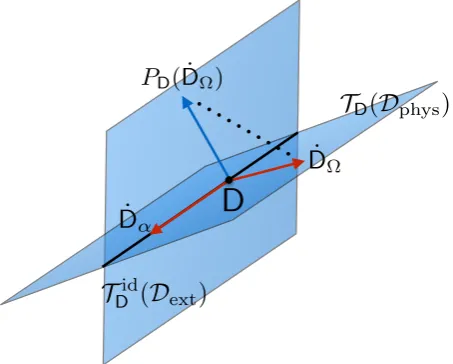
photons monitored on the environment. In addition, we include the above discussed phase shift θ to the emitted photons. The auxiliary parameters are chosen such that their tangent vectors lie in the identifiable subspace at v= 0; their span is needed in order to describe the horizontal projections of the physical tangent vectors, as we will see below.

The quantum Fisher information associated with the three parameters (∆,Ω, α) of this model has been compared with particular measurement strategies22_{; we emphasise geometric}

aspects not discussed there, and have also included the phase parameter θ. The main idea is to demonstrate how the rather complicated expressions of the Fisher information arise from considerably simpler geometric ingredients as a result of straightforward linear algebra. This provides insight on the structure of the physical system from the operational identification point of of view, and may eventually be useful in developing global estimation strategies in analogy to classical cases (see e.g.35).

Accordingly, we let _Dext denote the whole (extended) 7-dimensional manifold, and Dphys =