Effective parallelisation for machine learning

Effective Parallelisation for Machine Learning

Michael Kamp University of Bonn and Fraunhofer IAIS [email protected]

Mario Boley

Max Planck Institute for Informatics and Saarland University [email protected]

Olana Missura Google Inc. [email protected]

Thomas G¨artner University of Nottingham

[email protected]

Abstract

We present a novel parallelisation scheme that simplifies the adaptation of learn-ing algorithms to growlearn-ing amounts of data as well as growlearn-ing needs for accurate and confident predictions in critical applications. In contrast to other parallelisa-tion techniques, it can be applied to a broad class of learning algorithms without further mathematical derivations and without writing dedicated code, while at the same time maintaining theoretical performance guarantees. Moreover, our par-allelisation scheme is able to reduce the runtime of many learning algorithms to polylogarithmic time on quasi-polynomially many processing units. This is a sig-nificant step towards a general answer to an open question [21] on efficient paral-lelisation of machine learning algorithms in the sense of Nick’s Class (N C). The cost of this parallelisation is in the form of a larger sample complexity. Our empir-ical study confirms the potential of our parallelisation scheme with fixed numbers of processors and instances in realistic application scenarios.

1

Introduction

This paper contributes a novel and provably effective parallelisation scheme for a broad class of learning algorithms. The significance of this result is to allow the confident application of machine learning algorithms with growing amounts of data. In critical application scenarios, i.e., when errors have almost prohibitively high cost, this confidence is essential [27,36]. To this end, we consider the parallelisation of an algorithm to be effective if it achieves the same confidence and error bounds as the sequential execution of that algorithm in much shorter time. Indeed, our parallelisation scheme can reduce the runtime of learning algorithms from polynomial to polylogarithmic. For that, it consumes more data and is executed on a quasi-polynomial number of processing units.

To formally describe and analyse our parallelisation scheme, we consider the regularised risk min-imisation setting. For a fixed but unknown joint probability distributionDover aninput spaceX and anoutput spaceY, a datasetD⊆ X × Yof sizeN∈Ndrawn iid fromD, a convexhypothesis

spaceF of functionsf: X → Y, a loss function`:F × X × Y →_Rthat is convex inF, and a convex regularisation termΩ :F →R,regularised risk minimisation algorithmssolve

L(D) = argmin

f∈F

N

X

i=1

`(f, Xi, Yi) + Ω(f) . (1)

The aim of this approach is to obtain a hypothesisf ∈ Fwith smallregret Q(f) =E[`(f, X, Y)]−argmin

f0_∈F E

Regularised risk minimisation algorithms are typically designed to beconsistentandefficient. They are consistent if there is a functionN0:R+×R+→R+such that for allε >0,∆∈(0,1],N ∈N

withN ≥N0(ε,∆), and training dataD ∼ DN, the probability of generating anε-bad hypothesis is smaller than∆, i.e.,

P(Q(L(D))> ε)≤∆ . (3)

They are efficient if thesample complexityN0(ε,∆)is polynomial in1/ε,log1/∆and the runtime complexityTLis polynomial in the sample complexity. This paper considers the parallelisation of such consistent and efficient learning algorithms, e.g., support vector machines, regularised least squares regression, and logistic regression. We additionally assume that data is abundant and thatF can be parametrised in a fixed, finite dimensional Euclidean spaceRdsuch that the convexity of the

regularised risk minimisation problem (1) is preserved. In other cases, (non-linear) low-dimensional embeddings [2,28] can preprocess the data to facilitate parallel learning with our scheme. With slight abuse of notation, we identify the hypothesis space with its parametrisation.

The main theoretical contribution of this paper is to show that algorithms satisfying the above con-ditions can be parallelisedeffectively. We consider a parallelisation to be effective if the(ε, ∆)-guarantees (Equation3) are achieved in time polylogarithmic inN0(ε,∆). The cost for achieving this reduction in runtime comes in the form of an increased data size and through the number of processing units used. For the parallelisation scheme presented in this paper, we are able to bound this cost by a quasi-polynomial in1_/εandlog1_{/∆. The main practical contribution of this paper is} an effective parallelisation scheme that treats the underlying learning algorithm as ablack-box, i.e., it can be parallelised without further mathematical derivations and without writing dedicated code.

Similar to averaging-based parallelisations [32,44,45], we apply the underlying learning algorithm in parallel to random subsets of the data. Each resulting hypothesis is assigned to a leaf of an aggregation tree which is then traversed bottom-up. Each inner node computes a new hypothesis that is aRadon point[30] of its children’s hypotheses. In contrast to aggregation by averaging, the Radon point increases the confidence in the aggregate doubly-exponentially with the height of the aggregation tree. We describe our parallelisation scheme, called theRadon machine, in detail in Section2. Comparing the Radon machine to a sequential application of the underlying learning algorithm which achieves the same confidence, we are able to show a strong reduction in runtime from polynomial to polylogarithmic in Section3.

The empirical evaluation of the Radon machine in Section4confirms its potential in practical set-tings. Given the same data as the sequential application of the base learning algorithm, the Radon machine achieves a substantial reduction of computation time in realistic application scenarios. In particular, using150processors, the Radon machine is between80and around700-times faster than the base learner. Notice that superlinear speed-ups are possible for base learning algorithms with superlinear runtime. Compared with parallel learning algorithms from the Spark machine learning library, it achieves hypotheses of similar quality, while requiring only15−85%of their runtime.

Parallel computing [18] and its limitations [14] have been studied for a long time in theoretical com-puter science [7]. Parallelising polynomial time algorithms ranges from being ‘embarrassingly’ [26] easy to being believed to be impossible: For the class of decision problems that are the hardest in P, i.e., for P-complete problems, it is believed that there is no efficient parallel algorithm in the sense of Nick’s Class (NC [9]): efficient parallel algorithms in this sense are those that can be executed

Algorithm 1Radon Machine

Input: learning algorithmL, datasetD⊆ X × Y, Radon numberr∈N, and parameterh∈N

Output: hypothesisf ∈ F 1: divideDintorh_{iid subsetsD}

iof roughly equal size

2: runLin parallel to obtainfi=L(Di)

3: S ← {f1, . . . , frh}

4: fori=h−1, . . . ,1do

5: partitionSinto iid subsetsS1, . . . , Sriof sizereach

6: calculater(S1), . . . ,r(Sri)in parallel

7: S ← {r(S1), . . . ,r(Sri)}

inpolylogarithmic timeon apolynomial number of processing units. Our paper thus contributes to understanding the extent to which efficient parallelisation of polynomial time learning algorithms is possible. This connection and other approaches to parallel learning are discussed in Section5.

2

From Radon Points to Radon Machines

The Radon machine, as described in Algorithm 1, first executes the base learning algorithm on random subsets of the data to quickly achieve weak hypotheses and then iteratively aggregates them to stronger ones. Both the generation of weak hypotheses and the aggregation can be executed in parallel. To aggregate hypotheses, we follow along the lines of the iterated Radon point algorithm which was originally devised to approximate the centre point of a finite set of points [8]. The Radon point [30] of a set of points is defined as follows:

Definition 1. ARadon partitionof a setS ⊂ F is a pairA, B ⊂ S such thatA∩B = ∅but hAi ∩ hBi 6=∅, whereh·idenotes the convex hull. TheRadon numberof a spaceFis the smallest r∈Nsuch that for allS ⊂ Fwith|S| ≥rthere is a Radon partition, or∞if no Radon partition

exists. ARadon pointof a setSwith Radon partitionA, B⊂Sis anyr∈ hAi ∩ hBi.

We now present the Radon machinein Algorithm1, which is able to effectively parallelise consistent and efficient learning algorithms. Input to this parallelisation scheme is a learning algorithmLon a hypothesis spaceF, a datasetD ⊆ X × Y, the Radon numberr ∈ Nof the hypothesis space

F, and a parameterh∈N. It divides the dataset intorhsubsetsD1, . . . , Drh(line1) and runs the

algorithmLon each subset in parallel (line 2). Then, the set of hypotheses (line3) is iteratively aggregated to form better sets of hypotheses (line4-8). For that the set is partitioned into subsets of sizer(line5) and the Radon point of each subset is calculated in parallel (line6). The final step of each iteration is to replace the set of hypotheses by the set of Radon points (line7).

The scheme requires a hypothesis space with a valid notion of convexity and finite Radon number. While other notions of convexity are possible [16,33], in this paper we restrict our consideration to Euclidean spaces with the usual notion of convexity. Radon’s theorem [30] states that the Euclidean spaceRdhas Radon numberr = d+ 2. Radon points can then be obtained by solving a system

of linear equations of sizer×r(to be fully self-contained we state the system of linear equations explicitly in AppendixC.1). The next proposition gives a guarantee on the quality of Radon points:

Proposition 2. Given a probability measurePover a hypothesis spaceFwith finite Radon number r, letF denote a random variable with distributionP. Furthermore, letrbe the random variable obtained by computing the Radon point ofrrandom points drawn according toPr_{. Then it holds}

for the expected regretQand allε∈Rthat

P(Q(r)> ε)≤(rP(Q(F)> ε))2 .

A direct consequence of this proposition is a bound on the probability that the output of the Radon machine with parameterhis bad:

Theorem 3. Given a probability measureP over a hypothesis spaceFwith finite Radon number r, letF denote a random variable with distributionP. Furthermore, letrhbe the random variable

representing the Radon point obtained afterhiterations with base hypotheses drawn according to P. Then for any convex functionQ:F →_Rand allε∈_Rit holds that

P(Q(rh)> ε)≤(rP(Q(F)> ε))2

h

.

The proofs of Proposition 2and Theorem3 are provided in Section7. Note that this proof also shows the robustness of the Radon point compared to the average: if only one ofrpoints isε-bad, the Radon point is stillε-good, while the average may or may not be; indeed, in a linear space with any set ofε-good hypotheses and anyε0≥ε, we can always find a singleε0-bad hypothesis such that the average of all these hypotheses isε0-bad. For the Radon machine with parameterh, Theorem3 shows that the probability of obtaining anε-bad hypothesis is doubly exponentially reduced: with a boundδon this probability for the base learning algorithm, the bound∆for the Radon machine is

∆ = (rδ)2h . (4)

3

Sample and Runtime Complexity

In this section we first derive the sample and runtime complexity of the Radon machineRfrom the sample and runtime complexity of the base learning algorithmL. We then relate the runtime complexity of the Radon machine to a sequential application of the base learning algorithm when both achieve the the same(ε,∆)-guarantee. For that, we assume that the base learning algorithms is consistent and efficient with a sample complexity of the formN₀L(ε, δ) = (αε+βεld1/δ)k, for

some1_α

ε, βε∈R, andk∈N. We assume for the base learning algorithm thatδ≤1/2r.

The Radon machine createsrh_{base hypotheses and, with∆as in Equation4, has sample complexity}

N₀R(ε,∆) = rhN₀L(ε, δ) = rh·

αε + βεld

1 δ

k

. (5)

Theorem3then shows that the Radon machine with base learning algorithmLis consistent: with N ≥N₀R(ε,∆)samples it achieves an(ε,∆)-guarantee. To achieve the same guarantee, the appli-cation ofLitself, sequentially, would requireM ≥N0L(ε,∆)samples, where

N₀L(ε,∆) = N₀Lε,(rδ)2h =

αε + 2h·βεld

1 rδ

k

. (6)

For base learning algorithms L with runtime TL(n) polynomial in the data size n ∈ N, i.e.,

TL(n)∈ O(nκ)withκ∈N, we now determine the runtimeTR,h(N)of the Radon machine with

hiterations andc = rh_{processing units onN ∈}

Nsamples. In this case all base learning

algo-rithms can be executed in parallel. In practical applications fewer physical processors can be used to simulaterhprocessing units—we discuss this case in Section5.

The runtime of the Radon machine can be decomposed into the runtime of the base learning algo-rithm and the runtime for the aggregation. The base learning algoalgo-rithm requiresn ≥ N₀R(ε,∆)_/rh

samples and can be executed onrh_{processors in parallel in timeT}

L(n). The Radon point in each of thehiterations can then be calculated in parallel in timer3(see AppendixC.1). Thus, the runtime of the Radon machine withN=rh_{nsamples is}

TR,h(N) =TL(n) +hr3 . (7)

In contrast, the runtime of the base learning algorithm for achieving the same guarantee is TL(M)with M ≥ N0L(ε,∆). Ignoring logarithmic and constant terms, N0L(ε,∆) behaves as 2h_NL

0(ε, δ). To obtain polylogarithmic runtime ofRcompared toTL(M), we choose the parame-terh≈ldM−ld ldM such thatn≈M_/2h_{= ldM. Thus, the runtime of the Radon machine is in}

O ldκM +r3_ldM

. This result is formally summarised in Theorem4.

Theorem 4. The Radon machine with a consistent and efficient regularised risk minimisation al-gorithm on a hypothesis space with finite Radon number has polylogarithmic runtime on quasi-polynomially many processing units if the Radon number is upper bounded by a function polyloga-rithmic in the sample complexity of the efficient regularised risk minimisation algorithm.

The theorem is proven in AppendixA.1and relates to Nick’s Class [1]: A decision problem can be solved efficiently in parallel in the sense of Nick’s Class, if it can be decided by an algorithm in polylogarithmic time on polynomially many processors (assuming, e.g., PRAM model). For the class of decision problems that are the hardest inP, i.e., forP-complete problems, it is believed that there is no efficient parallel algorithm for solving them in this sense. Theorem4 provides a step towards finding efficient parallelisations of regularised risk minimisers and towards answering the open question: is consistent regularised risk minimisation possible in polylogarithmic time on polynomially many processors. A similar question, for the case of learning half spaces, has been coined a fundamental open problem by Long and Servedio [21] who gave an algorithms which runs on polynomially many processors in time that depends polylogarithmically on the sample size but is inversely proportional to a parameter of the learning problem. While Nick’s Class as a notion of efficiency has been criticised, e.g., by Kruskal et al. [17], it is the only notion of efficiency that forms a proper complexity class, in the sense of Blum [4]. Additionally, Kruskal et al. [17] suggested to also consider the inefficiency of simulating the parallel algorithm on a single processing unit. We consider this in AppendixA.2, where we also discuss the speed-up [17] usingcprocessing units.

1

4

Empirical Evaluation

This empirical study compares the Radon machine to state-of-the-art parallel machine learning al-gorithms from the Spark machine learning library [25], as well as the natural baseline of averaging hypotheses instead of calculating their Radon point (denoted averaging-at-the-end). In this study, we use base learning algorithms from WEKA [43] and scikit-learn [29]. We compare the Radon machine to the base learning algorithms on moderately sized datasets, due to scalability limitations of the base learners, and reserve larger datasets for the comparison with parallel learners. The exper-iments are executed on a Spark cluster (5worker nodes,25processors per node)2. In this study, we apply the Radon machine with parameterh= 1and the maximal parameterh(denotedh=max) such that each instance of the base learning algorithm is executed on a subset of size at least100. Averaging-at-the-end uses the same parameterhand executes the base learning algorithm onrh_of

subsets, i.e., the same number as the Radon machine with that parameter.

What is the speed-up of our scheme in practice? In Figure1(a), we compare the Radon ma-chine to its base learners on moderately sized datasets (details on the datasets are provided in Appendix B). There, the Radon machine is is between80 and around700-times faster than the base learner, using150 processors. The speed-up is detailed in Figure2. On the SUSY dataset

2

The source code implementation in Spark can be found in the bitbucket repository

https://bitbucket.org/Michael_Kamp/radonmachine. 102 103 104 105 106

training time (log-scale)

WekaSGD WekaLogReg LinearSVC PRM(h=1)[WekaSGD] PRM(h=1)[WekaLogReg] PRM(h=1)[LinearSVC] PRM(h=max)[WekaSGD] PRM(h=max)[WekaLogReg] PRM(h=max)[LinearSVC]

codrna _Stagger1 SEA_50 poker

click_pred SUSY 0.0 0.2 0.4 0.6 0.8 1.0 AUC (a) 102 103 104 105 Avg(h=1)[WekaSGD] Avg(h=max)[WekaSGD] Avg(h=1)[WekaLogReg] Avg(h=max)[WekaLogReg] PRM(h=1)[WekaSGD] PRM(h=1)[WekaLogReg] PRM(h=max)[WekaSGD] PRM(h=max)[WekaLogReg]

20_news SUSY HIGGS wikidata CASP9

0.0 0.2 0.4 0.6 0.8 1.0 (b) 102 103 104 105 SparkLogRegwSGD SparkSVMwSGD SparkLogRegwLBFGS SparkLogReg PRM(h=1)[WekaSGD] PRM(h=1)[WekaLogReg] PRM(h=max)[WekaSGD] PRM(h=max)[WekaLogReg]

20_news SUSY HIGGS wikidata CASP9

0.0 0.2 0.4 0.6 0.8 1.0 (c)

poker

Stagger1 SEA_50 SUSY _{click_pred} codrna

101 102 103 speedup WekaSGD WekaLogReg LinearSVC

Figure 2: Speed-up (log-scale) of the Radon machine over its base learners per dataset from the same experiment as in Figure1(a).

106 ₁₀7

dataset size 103 104 105 106 runtime 1.57 1.17 central Radon

Figure 3: Dependence of the runtime on the dataset size for of the Radon machine com-pared to its base learners.

103 ₁₀4

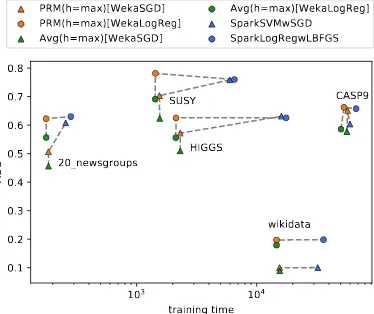
training time 0.1 0.2 0.3 0.4 0.5 0.6 0.7 0.8 AUC 20_newsgroups SUSY HIGGS wikidata CASP9 PRM(h=max)[WekaSGD] PRM(h=max)[WekaLogReg] Avg(h=max)[WekaSGD] Avg(h=max)[WekaLogReg] SparkSVMwSGD SparkLogRegwLBFGS

Figure 4: Representation of the results in Fig-ure1(b)and1(c)in terms of the trade-off between runtime and AUC for the Radon machine (PRM) and averaging-at-the-end (Avg), both with param-eterh= max, and parallel machine learning al-gorithms in Spark.

(with 5 000 000 instances and 18 features), the Radon machine on 150 processors with h= 3 is 721 times faster than its base learn-ing algorithms. At the same time, their practi-cal performances, measured by the area under the ROC curve (AUC) on an independent test dataset, are comparable.

How does the scheme compare to averaging-at-the-end? In Figure 1(b) we compare the runtime and AUC of the parallelisation scheme against theAvgbaseline. Since averaging is less computationally expensive than calculating the Radon point, the runtimes of the Avg baselines are slightly lower than the ones of the Radon machine. However, compared to the computa-tional complexity of executing the base learner, this advantage becomes negligible. In terms of AUC, the Radon machine outperforms the av-eraging baseline on all datasets by at least10%.

How does our scheme compare to state-of-the-art Spark machine learning algorithms? We compare the Radon machine to various Spark machine learning algorithms on 5large

How does the runtime depend on the dataset size in a real-world system? In Figure 3 we compare the runtimes of all base learning algorithms per dataset size to the Radon machines. Results indicate that, while the runtimes of the base learning algorithms depends on the dataset size with an average exponent of1.57, the runtime of the Radon machine depends on the dataset size with an exponent of only1.17. This is plausible because with enough processors the generation of weak hypotheses can be done completely in parallel. Moreover, the time for aggregating the hypotheses does not depend on the number of instances in the dataset, but only on the number of iterations and the dimension of the hypothesis space.

How generally applicable is the scheme?As an indication of the general applicability in practice, we apply the scheme to an Scikit-learn implementation of regularised least squares regression [29]. On the datasetYearPredictionMSD, regularised least squares regression achieves an RMSE of12.57, whereas the Radon machine achieved an RMSE of13.64. At the same time, the Radon machine is 197-times faster. We also compare the Radon machine on a multi-class prediction problem using conditional maximum entropy models. We use the implementation described in Mcdonald et al. [23], who also propose to use averaging-at-the-end for distributed training. We compare the Radon machine to averaging-at-the-end with conditional maximum entropy models on two large multi-class datasets (driftandspoken-arabic-digit). On average, our scheme performs4%better with only 0.2%longer runtime. The minimal difference in runtime can be explained—similar to the results in Figure1(b)—by the smaller complexity of calculating the average instead of the Radon point.

5

Discussion and Related Work

In this paper we provided a step towards answering an open problem: Is parallel machine learn-ing possible in polylogarithmic time uslearn-ing a polynomial number of processors only? This question has been posed for half-spaces by Long and Servedio [21] and called “a fundamental open prob-lem about the abilities and limitations of efficient parallel learning algorithms”. It relates machine learning to Nick’s Class of parallelisable decision problems and its variants [14]. Early theoretical treatments of parallel learning with respect to NC consideredprobably approximately correct(PAC) [5, 38] concept learning. Vitter and Lin [41] introduced the notion ofNC-learnable for concept classes for which there is an algorithm that outputs a probably approximately correct hypothesis in polylogarithmic time using a polynomial number of processors. In this setting, they proved positive and negative learnability results for a number of concept classes that were previously known to be PAC-learnable in polynomial time. More recently, the special case of learning half spaces in par-allel was considered by Long and Servedio [21] who gave an algorithm for this case that runs on polynomially many processors in time that depends polylogarithmically on the size of the instances but is inversely proportional to a parameter of the learning problem. Our paper complements these theoretical treatments of parallel machine learning and provides a provably effective parallelisation scheme for a broad class of regularised risk minimisation algorithms.

Some parallelisation schemes also train learning algorithms on small chunks of data and average the found hypotheses. While this approach has advantages [13,32], current error bounds do not allow a derivation of polylogarithmic runtime [20,35,44] and it has been doubted to have any benefit over learning on a single chunk [34]. Another popular class of parallel learning algorithms is based on stochastic gradient descent, targeting expected risk minimisation directly [34, and references therein]. The best, so far known algorithm in this class [34] is the distributed mini-batch algorithm [10]. This algorithm still runs for a number of rounds inversely proportional to the desired opti-misation error, hence not in polylogarithmic time. A more traditional approach is to minimise the empirical risk, i.e., an empirical sample-based approximation of the expected risk, using any, deter-ministic or randomised, optimisation algorithm. This approach relies on generalisation guarantees relating the expected and empirical risk minimisation as well as a guarantee on the optimisation error introduced by the optimisation algorithm. The approach is readily parallelisable by employing avail-able parallel optimisation algorithms [e.g.,6]. It is worth noting that these algorithms solve a harder than necessary optimisation problem and often come with prohibitively high communication cost in distributed settings [34]. Recent results improve over these [22] but cannot achieve polylogarithmic time as the number of iterations depends linearly on the number of processors.

In the experiments we considered datasets where the number of dimensions is much smaller than the number of instances. What about high-dimensional models? The basic version of the paral-lelisation scheme presented in this paper cannot directly be applied to cases in which the size of the dataset is not at least a multiple of the Radon number of the hypothesis space. For various types of data such as text, this might cause concerns. However, random projections [15] or low-rank approx-imations [2,28] can alleviate this problem and are already frequently employed in machine learning. An alternative might be to combine our parallelisation scheme with block coordinate descent [37]. In this case, the scheme can be applied iteratively to subsets of the features.

In the experiments we considered only linear models. What about non-linear models? Learning non-linear models causes similar problems to learning high-dimensional ones. In non-parametric methods like kernel methods, for instance, the dimensionality of the optimisation problem is equal to the number of instances, thus prohibiting the application of our parallelisation scheme. However, similar low-rank approximation techniques as described above have been applied with non-linear kernels [11]. Alternatively, novel methods for speeding up the learning process for non-linear mod-els rely on explicitly constructing an embedding in which a linear model can be learned [31]. Using explicitly constructed feature spaces, Radon machines can directly be applied to non-linear models.

We have theoretically analysed our parallelisation scheme for the case that there are enough proces-sors available to find each weak hypothesis on a separate processor.What if there are less thanrh

processors?The parallelisation scheme can quite naturally be de-parallelised and partially executed in sequence. For the runtime this implies an additional factor ofmax{1,rh/c}. Thus, the Radon

ma-chine can be applied with any number of processors.

The scheme improves the confidence∆doubly exponentially in its parameterhbut for that it re-quires the weak hypotheses to already achieve a base confidence of1−δ >1−1_{/2r.Is the scheme} only applicable in high-confidence domains?Many application scenarios require high-confidence error bounds, e.g., in the medical domain [27] or in intrusion detection [36]. Apart from these theoretical considerations, in practice our scheme performs comparably to its base learner.

Besides runtime, communication plays an essential role in parallel learning. What is the commu-nication complexity of the scheme?As for all aggregation at the end strategies, the overall amount of communication is low compared to periodically communicating schemes. For the parallel aggre-gation of hypotheses, the scheme requiresO(rh+1_{)messages each containing a single hypothesis} of sizeO(d). Furthermore, only a fraction of the data has to be transferred to each processor. Our scheme is ideally suited for inherently distributed data.

6

Conclusion and Future Work

We have proposed a parallelisation scheme that is effective, i.e., it speeds up computation through parallelisation while achieving the same hypothesis quality as the base learner. It is a black-box parallelisation in the sense that it is applicable to a wide range of machine learning algorithms and is oblivious to the implementation of these algorithms. Our empirical evaluation shows that in practice substantial speed-ups are achieved by the Radon machine.

7

Proof of Proposition

2

and Theorem

3

In order to prove Proposition2and consecutively Theorem3, we require the following properties of Radon points and convex functions. We proof these properties for the more general case of quasi-convex functions. Since every quasi-convex function is also quasi-quasi-convex, the results hold for quasi-convex functions as well. A quasi-convex function is defined as follows.

Definition 5. A functionQ:F →Ris calledquasi-convexif all its sublevel sets are convex, i.e.,

∀θ∈R:{f ∈ F |Q(f)< θ}is convex.

First we give a different characterisation of quasi-convex functions.

Proposition 6. A functionQ :F →Ris quasi-convex⇔ ∀S ⊆ F,∀s0 ∈ hSi,∃s∈S :Q(s)≥

Q(s0).

Proof.

(⇒) Suppose this direction does not hold. Then there is a convex functionQ, a setS ⊆ F, and ans0 ∈ hSisuch that for alls ∈ S it holds thatQ(s) <Q(s0)(therefores0 ∈/ S). Let C={c∈ F | Q(c)<Q(s0)}. AsS⊆Cwe also have thathSi ⊆ hCiwhich contradicts hSi 3s0∈/C.

(⇐) Suppose this direction does not hold. Then there exists an ε such that S={s∈ F | Q(s)< ε} is not convex and there is ans0 ∈ hSi \S. By assumption ∃s∈S :Q(s)≥ Q(s0). HenceQ(s0)< εand we have a contradiction since this would implys0 ∈S.

The next proposition concerns the value of any convex function at a Radon point.

Proposition 7. For every setSwith Radon pointrand every quasi-convex functionQit holds that |{s∈S| Q(s)≥ Q(r)}| ≥2.

Proof. We show a slightly stronger result: Take any family of pairwise disjoint sets Ai with

T

ihAii 6= ∅ andr ∈ TihAii. From proposition 6follows directly the existence of anai ∈ Ai

such thatQ(ai)≥ Q(r). The desired result follows then fromai6=aj⇐i6=j.

Using this property, we can proof Proposition2and Theorem3.

Proof of Proposition2and Theorem3. By proposition 7, for any Radon pointr of a setS there must be two pointsa, b∈SwithQ(a),Q(b)≥ Q(r). Henceforth, the probability ofQ(r)> εis smaller or equal than the probability of the paira, bhavingQ(a),Q(b)> ε. Proposition2follows by an application of the union bound on all pairs fromS. Repeated application of the proposition proves Theorem3.

Acknowledgements

References

[1] Sanjeev Arora and Boaz Barak. Computational complexity: A modern approach. Cambridge University Press, 2009.

[2] Maria Florina Balcan, Yingyu Liang, Le Song, David Woodruff, and Bo Xie. Communication efficient distributed kernel principal component analysis. In Proceedings of the 22nd ACM SIGKDD International Conference on Knowledge Discovery and Data Mining, pages 725– 734, 2016.

[3] Peter L. Bartlett and Shahar Mendelson. Rademacher and gaussian complexities: Risk bounds and structural results. Journal of Machine Learning Research, 3:463–482, 2003.

[4] Manuel Blum. A machine-independent theory of the complexity of recursive functions. Jour-nal of the ACM (JACM), 14(2):322–336, 1967.

[5] Anselm Blumer, Andrzej Ehrenfeucht, David Haussler, and Manfred K Warmuth. Learnability and the Vapnik-Chervonenkis dimension.Journal of the ACM (JACM), 36(4):929–965, 1989.

[6] Stephen Boyd, Neal Parikh, Eric Chu, Borja Peleato, and Jonathan Eckstein. Distributed op-timization and statistical learning via the alternating direction method of multipliers. Founda-tions and Trends® in Machine Learning, 3(1):1–122, 2011.

[7] Ashok K. Chandra and Larry J. Stockmeyer. Alternation. In 17th Annual Symposium on Foundations of Computer Science, pages 98–108, 1976.

[8] Kenneth L. Clarkson, David Eppstein, Gary L. Miller, Carl Sturtivant, and Shang-Hua Teng. Approximating center points with iterative Radon points. International Journal of Computa-tional Geometry & Applications, 6(3):357–377, 1996.

[9] Stephen A. Cook. Deterministic CFL’s are accepted simultaneously in polynomial time and log squared space. InProceedings of the eleventh annual ACM symposium on Theory of computing, pages 338–345, 1979.

[10] Ofer Dekel, Ran Gilad-Bachrach, Ohad Shamir, and Lin Xiao. Optimal distributed online prediction using mini-batches. Journal of Machine Learning Research, 13(1):165–202, 2012.

[11] Shai Fine and Katya Scheinberg. Efficient svm training using low-rank kernel representations. Journal of Machine Learning Research, 2:243–264, 2002.

[12] Yoav Freund. Boosting a weak learning algorithm by majority.Information and computation, 121(2):256–285, 1995.

[13] Yoav Freund, Yishay Mansour, and Robert E. Schapire. Why averaging classifiers can protect against overfitting. InProceedings of the 8th International Workshop on Artificial Intelligence and Statistics, 2001.

[14] Raymond Greenlaw, H. James Hoover, and Walter L. Ruzzo. Limits to parallel computation: P-completeness theory. Oxford University Press, Inc., 1995.

[15] William B. Johnson and Joram Lindenstrauss. Extensions of lipschitz mappings into a hilbert space. Contemporary mathematics, 26(189-206):1, 1984.

[16] David Kay and Eugene W. Womble. Axiomatic convexity theory and relationships between the Carath´eodory, Helly, and Radon numbers. Pacific Journal of Mathematics, 38(2):471–485, 1971.

[17] Clyde P. Kruskal, Larry Rudolph, and Marc Snir. A complexity theory of efficient parallel algorithms.Theoretical Computer Science, 71(1):95–132, 1990.

[19] Moshe Lichman. UCI machine learning repository, 2013. URLhttp://archive.ics. uci.edu/ml.

[20] Shao-Bo Lin, Xin Guo, and Ding-Xuan Zhou. Distributed learning with regularized least squares. Journal of Machine Learning Research, 18(92):1–31, 2017. URLhttp://jmlr.

org/papers/v18/15-586.html.

[21] Philip M. Long and Rocco A. Servedio. Algorithms and hardness results for parallel large margin learning.Journal of Machine Learning Research, 14:3105–3128, 2013.

[22] Chenxin Ma, Jakub Koneˇcn´y, Martin Jaggi, Virginia Smith, Michael I. Jordan, Peter Richt´arik, and Martin Tak´aˇc. Distributed optimization with arbitrary local solvers.Optimization Methods and Software, 32(4):813–848, 2017.

[23] Ryan Mcdonald, Mehryar Mohri, Nathan Silberman, Dan Walker, and Gideon S. Mann. Effi-cient large-scale distributed training of conditional maximum entropy models. InAdvances in Neural Information Processing Systems, pages 1231–1239, 2009.

[24] Brendan McMahan, Eider Moore, Daniel Ramage, Seth Hampson, and Blaise Aguera y Ar-cas. Communication-efficient learning of deep networks from decentralized data. InArtificial Intelligence and Statistics, pages 1273–1282, 2017.

[25] Xiangrui Meng, Joseph Bradley, Burak Yavuz, Evan Sparks, Shivaram Venkataraman, Davies Liu, Jeremy Freeman, DB Tsai, Manish Amde, Sean Owen, Doris Xin, Reynold Xin, Michael J. Franklin, Reza Zadeh, Matei Zaharia, and Ameet Talwalkar. Mllib: Machine learn-ing in apache spark.Journal of Machine Learning Research, 17(34):1–7, 2016.

[26] Cleve Moler. Matrix computation on distributed memory multiprocessors. Hypercube Multi-processors, 86(181-195):31, 1986.

[27] Ilia Nouretdinov, Sergi G. Costafreda, Alexander Gammerman, Alexey Chervonenkis, Vladimir Vovk, Vladimir Vapnik, and Cynthia H.Y. Fu. Machine learning classification with confidence: application of transductive conformal predictors to MRI-based diagnostic and prognostic markers in depression.Neuroimage, 56(2):809–813, 2011.

[28] Dino Oglic and Thomas G¨artner. Nystr¨om method with kernel k-means++ samples as land-marks. In Proceedings of the 34th International Conference on Machine Learning, pages 2652–2660, 06–11 Aug 2017.

[29] Fabian Pedregosa, Ga¨el Varoquaux, Alexandre Gramfort, Vincent Michel, Bertrand Thirion, Olivier Grisel, Mathieu Blondel, Peter Prettenhofer, RRon Weiss, Vincent Dubourg, Jake Vanderplas, AAlexandre Passos, David Cournapeau, Matthieu Brucher, Matthieu Perrot, and

´

Edouard Duchesnay Duchesnay. Scikit-learn: Machine learning in Python.Journal of Machine Learning Research, 12:2825–2830, 2011.

[30] Johann Radon. Mengen konvexer K¨orper, die einen gemeinsamen Punkt enthalten. Mathema-tische Annalen, 83(1):113–115, 1921.

[31] Ali Rahimi and Benjamin Recht. Random features for large-scale kernel machines. In Ad-vances in Neural Information Processing Systems, pages 1177–1184, 2007.

[32] Jonathan D. Rosenblatt and Boaz Nadler. On the optimality of averaging in distributed statis-tical learning. Information and Inference, 5(4):379–404, 2016.

[33] Alexander M. Rubinov. Abstract convexity and global optimization, volume 44. Springer Science & Business Media, 2013.

[34] Ohad Shamir and Nathan Srebro. Distributed stochastic optimization and learning. In Proceed-ings of the 52nd Annual Allerton Conference on Communication, Control, and Computing, pages 850–857, 2014.

[36] Robin Sommer and Vern Paxson. Outside the closed world: On using machine learning for network intrusion detection. InSymposium on Security and Privacy, pages 305–316, 2010.

[37] Suvrit Sra, Sebastian Nowozin, and Stephen J. Wright. Optimization for machine learning. MIT Press, 2012.

[38] Leslie G. Valiant. A theory of the learnable.Communications of the ACM, 27(11):1134–1142, 1984.

[39] Joaquin Vanschoren, Jan N. van Rijn, Bernd Bischl, and Luis Torgo. OpenML: Networked science in machine learning. SIGKDD Explorations, 15(2):49–60, 2013.

[40] Vladimir N. Vapnik and Alexey Y. Chervonenkis. On the uniform convergence of relative frequencies of events to their probabilities. Theory of Probability & Its Applications, 16(2): 264–280, 1971.

[41] Jeffrey S. Vitter and Jyh-Han Lin. Learning in parallel. Information and Computation, 96(2): 179–202, 1992.

[42] Ulrike Von Luxburg and Bernhard Sch¨olkopf. Statistical learning theory: models, concepts, and results. InInductive Logic, volume 10 ofHandbook of the History of Logic, pages 651– 706. Elsevier, 2011.

[43] Ian H. Witten, Eibe Frank, Mark A. Hall, and Christopher J. Pal. Data Mining: Practical machine learning tools and techniques. Elsevier, 2017.

[44] Yuchen Zhang, John C. Duchi, and Martin J. Wainwright. Communication-efficient algorithms for statistical optimization.Journal of Machine Learning Research, 14(1):3321–3363, 2013.