Estimation of functional sparsity in nonparametric varying coefficient models for longitudinal data analysis

Estimation of Functional Sparsity in Nonparametric Varying

Coefficient Models for Longitudinal Data Analysis

Catherine Y. Tu1_{, Juhyun Park}2_{, and Haonan Wang}1 1_{Colorado State University,}2_{Lancaster University}

Abstract

We study the simultaneous domain selection problem for varying coefficient models as a

func-tional regression model for longitudinal data with many covariates. The domain selection problem

in functional regression mostly appears under the functional linear regression with scalar response,

but there is no direct correspondence to functional response models with many covariates. We

reformulate the problem as nonparametric function estimation under the notion offunctional spar-sity. Sparsity is the recurrent theme that encapsulates interpretability in the face of regression with multiple inputs, and the problem of sparse estimation is well understood in the parametric setting

as variable selection. For nonparametric models, interpretability not only concerns the number of

covariates involved but also thefunctional form of the estimates, and so the sparsity consideration is much more complex. To distinguish the types of sparsity in nonparametric models, we call the

former global sparsity and the latter local sparsity, which constitute functional sparsity. Most ex-isting methods focus on directly extending the framework of parametric sparsity for linear models

to nonparametric function estimation to address one or the other, but not both. We develop a

penalized estimation procedure that simultaneously addresses both types of sparsity in a unified

framework. We establish asymptotic properties of estimation consistency and sparsistency of the

proposed method. Our method is illustrated in simulation study and real data analysis, and is shown

to outperform the existing methods in identifying both local sparsity and global sparsity.

Keywords: Functional sparsity, Group bridge, Longitudinal data, Model selection, Nonpara-metric regression

1

Introduction

We study the simultaneous domain selection problem for varying coefficient models as a functional

multiple subjects with multiple predictors. The varying coefficient models [5,6] are defined as

y(t) =xT(t)β(t) +(t), (1.1)

wherey(t) is the response at timet,x(t) = (x1(t), . . . , xp(t))T is the vector of predictors at timet,(t) is

an error process independent ofx(t) andβ(t) = (β1(t), . . . , βp(t))T is a vector of time varying regression

coefficient functions. This model assumes a linear relationship between the response and predictors at

each observation time point but allows the coefficients to vary over time, thus greatly enhances the

utility of the standard linear model formulation. For generality, we write as if the predictors are also

functional, but note that the varying coefficient models are equally applicable when the predictors are

scalar valued, and our methodology developed here can be directly applied.

The domain selection problem in functional regression is known to be intrinsically difficult [15].

So far the problem is mostly studied in functional linear regression with a scalar response and single

functional covariate. Hall and Hooker [4] formulated the problem as a truncated regression model

with single unknown domain, studying the identifiability issues and nonparametric function estimation

problem. James et al. [11] on the other hand approached the problem from the viewpoint of sparsity

estimation as interpretable solutions. Using grid approximation, they imposed parametric sparsity

constraints on the derivatives of the underlying function at a large number of grid points, which

produces an estimate that distinguishes zero and non-zero regions. As Zhou et al. [30] noted, due

to overlapping contribution of each coefficient to neighboring regions, independent shrinkage of the

coefficients does not necessarily induce zero values in the coefficient function in general, and thus the

procedure tends to over-penalize. As a remedy, Zhou et al. [30] further suggested a two-step estimation

procedure. Wang and Kai [22] studied a similar problem under standard nonparametric regression,

suggesting the need of distinguishingfunctional features from parametric variable selection.

We consider the regression problem underfunctional responsevariable with varying coefficient

mod-els involving multiple domain selection under the general setting where the true number of covariates

is also unknown. Although the views and approaches taken in the earlier development are quite

dif-ferent, the problem of domain selection could be motivated as a means to enhance interpretability in

the face of model selection in nonparametric models. In this regard, we share the view that some

form of sparsity consideration could be useful. For nonparametric models, however, interpretability

not only concerns the number of covariates involved [16,24,25,27] but also the functional formof the

estimates [11, 30]. To distinguish the types of sparsity in nonparametric models, we call the former

a function hasglobal sparsityif it is zero over the entire domain, and it indicates that the corresponding

covariate is irrelevant to the response variable. A function haslocal sparsityif it is nonzero but remains

zero for a set of intervals, and it identifies an inactive period of the corresponding covariate. These

notions as interpretability were informally used in a rather separate context of the analysis, and thus

the significance of local sparsity estimation was not well recognized.

We reformulate the domain selection problem as a nonparametric function estimation under the

unified theme offunctional sparsity and propose a one-step penalized estimation procedure that

auto-matically determines the types of functional sparsity, being local or global. Although we distinguish

the two types of sparsity in the conceptual level, our unified formulation does not require distinction

between them in implementation. We directly exploit the fact that global sparsity is a special case of

local sparsity in view of domain selection, but not the other way around. Furthermore, consistency

of coefficient function estimation does not necessarily give information on local sparsity. This feature

distinguishes our approach from the majority methods targeting global sparsity such as [25]. It is

worth noting that there is a fundamental difference in the underlying assumption on sparsity between

parametric and nonparametric models, as our focus is on dense function estimation with dependent

variables with unknown domain. This difference was also recognized by Kneip et al. [12]. Moreover,

for parametric sparsity, an underlying sparse vector is specified whereas for functional sparsity itstrue

sparse representation may not be well defined in their respective function approximation. These

dif-ferences are not only philosophical, but pose different conceptual challenges in the development. Our

proposed penalized procedure resembles a type of parametric sparsity estimation, however, our analysis

is not comparable to those with high dimensional parametric sparsity estimation point of view (e.g.,

[11]).

We provide a theoretical analysis of the proposed method and, in particular, show that the local

sparsity can be consistently recovered, even diluted with the problem of global sparsity estimation. We

study the properties of our proposed method under standard assumptions on nonparametric smooth

function estimation and exploit the functional property in more natural manner, thus contribute to

bridging the gap between parametric variable selection and nonparametric functional sparsity in a

coherent manner.

Our formulation is given in Section 2. Our approach is a one-step procedure, and allows us to

directly control functional sparsity through the coefficient functions themselves, rather than pointwise

evaluation. In Section3, we study large sample properties of the proposed method and establish

scenarios, and a real data analysis is given in Section5, demonstrating the utility of functional sparsity

in relation to interpretability of the results. Technical assumptions and proofs are provided in the

online supplement.

2

Methodology

Suppose that, fornrandomly selected subjects, observations of thekth subject are obtained at{tkl, l=

1, . . . , nk}, and the measurements satisfy the varying coefficient linear model relationship in (1.1)

yk(tkl) =xT_k(tkl)β(tkl) +k(tkl), (2.1)

wherexk(tkl) = (x1(tkl), . . . , xp(tkl))T and yk(tkl) is the response of the kth subject attkl. We assume

that βi(t), i = 1, . . . , p are smooth coefficient functions with bounded second derivatives for t ∈ T.

We use spline approximations to represent β(t) and formulate a constrained optimization problem for

parameter estimation.

2.1 Least squares estimation under B-spline approximation

B-spline approximation has been widely used for estimating smooth nonparametric functions. For

detailed discussion about B-splines, see de Boor [2] and Schumaker [17]. Specifically, for a smooth

functionβ(t), t∈[0,1], its approximant can be written as

e β(t) =

J X

j=1

αjBj(t), (2.2)

where {Bj(·), j = 1, . . . , J} is a group of B-spline basis functions of degree d≥1 and knots 0 =η0 <

η1 < . . . < ηK < ηK+1= 1. Notice that K is the number of interior knots andJ =K+d+ 1. Here we

adopt the definition of B-spline as stated in Definition 4.12 of Schumaker [17]. In general, performance

of B-spline approximation has been well studied. For instance, under some mild conditions, there exists

a function βe(t) of the form (2.2) such that the approximation error goes to zero. See Theorem 6.27 of

Schumaker [17] for more details.

We write the B-spline approximation for each smooth nonparametric coefficient function as

e βi(t) =

Ji

X

j=1

whereBi(t) = (Bi1(t), . . . , BiJi(t))

T_,α

i = (αi1, . . . , αiji)

T _{and J}

i =Ki+d+ 1. HereKi is the number

of interior knots for βie(t) which may vary over i. For simplicity, we assume that the knots are evenly

distributed over [0,1]. Define a block diagonal matrix B(t) as

B(t) = diag{BT₁(t), . . . ,B_pT(t)}.

Using (2.3) in the varying coefficient model (2.1) leads to

yk(tkl)≈xTk(tkl)B(tkl)α+k(tkl) =Uk(tkl)α+k(tkl)

where Uk(tkl) =xT_k(tkl)B(tkl) andα = (αT1, . . . ,αTp)T. The least squares criterion of α [9] is defined

as

`(α) =

n X

k=1

ωkkyk−Ukαk22

whereyk = (yk(tk1), . . . , yk(tknk))

T _{and U}

k= (UkT(tk1), . . . ,UkT(tknk))

T_{. Weights ω}

k,k= 1, . . . , n, are

usually chosen as ωk ≡ 1 or ωk ≡ 1/nk [10]. In this paper, for simplicity, we set equal weights to

every subject, i.e., ωk ≡ 1. Putting U = (U1T, . . . ,UnT)T and y = (y1T, . . . ,ynT)T, the least squares

criterionl(α) can be written in matrix form; that is,l(α) =ky−U αk2

2. Huang et al. [10] proved that,

under certain assumptions, the matrix UTU is invertible for fixedp. Consequently, l(α) has a unique

minimizer

b

αLSE = (UTU)−1UTy,

which is the least squares estimator ofα, and thus, the least squares estimators of coefficient functions

are

b

β_iLSE(t) =

Ji

X

j=1 b

αLSE_ij Bij(t), i= 1, . . . , p,

whereαb

LSE

ij ’s are entries ofαLSEb . Here, we take marginal approach [26] to construct the LSE criterion

without accounting for within subject correlation. Proper modeling of covariance structure would

require further parametric assumptions [3] or nonparametric smoothing techniques [26], which is not

the focus of this paper.

2.2 B-spline approximation and Sparsity

From the B-spline approximation theory, there exists a function of the form (2.2) which is very close to

the true underlying function. While, this function is not capable of characterizing functional sparsity of

the true function. Here the term “functional sparsity” is a generalization of the “parameter sparsity”

0 0.1 0.2 0.3 0.4 0.5 0.6 0.7 0.8 0.9 1 −5

0 5 10

0 0.1 0.2 0.3 0.4 0.5 0.6 0.7 0.8 0.9 1 0

0.5 1

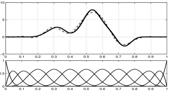
Figure 1: Top: a graphical display of a smooth function (solid thick line type) and two approximating

functions from a family of cubic B-spline basis functions with 9 equally-spaced interior knots. Bottom:

a graphical display of the set of B-spline functions used in the approximation.

For better illustration, we consider a toy example in Figure 1. Here, in the top panel, a smooth

functionβ(t) (thick line) with two spline approximants (dashed, dottted) are depicted. In the bottom,

a family of cubic B-spline basis functions with 9 interior knots is shown. The “best” fitted function from

theL2 criterion is shown as the dashed line in the upper panel, which signifies a good performance of

the approximation. We further note that β(t) is zeros on [0,0.1] and [0.9,1]; while, its approximation

is not zero except for some singletons. From that aspect, this approximation does not capture the

sparsity of the true underlying function. In contrast, the dotted curve depicted in the upper panel,

also a linear combination of the B-spline basis functions,automatically correctsthe function to preserve

local sparsity with almost indistinguishable performance.

The other extreme case arises when the function is close to zero, for part or the whole of the

interval. Our goal is to pursue a sparse solution, up to function approximation error, within the linear

space spanned by B-spline basis functions. From nonparmetric estimation viewpoint, such solution

preserves statistical accuracy and enhances interpretability; in fact, it is indistinguishable from the

true underlying function.

Inspired by above observations on functional sparsity, we develop a new procedure that equips

the least squares criterion with a regularization term. Usually, the regularization on parameters is

approximation of the coefficient functions.

2.3 Penalized Least Squares Estimation with Composite Penalty

It is not too difficult to see that global sparsity corresponds to group variable selection ofαi as a whole.

To achieve local sparsity, these estimates need to be adjusted in such a way that some of the estimates

could be exactly zero. As demonstrated in Section 2.2, we notice that for B-spline approximation,

when αj = 0 for j =l, . . . , l+d, the approximation βe(t) = 0 on the interval [ηl−1, ηl), and especially,

when αj = 0 for all j, βe(t) = 0 over the entire domain of [0, M]. This suggests local sparsity need

to be imposed at the level of a group of neighboring coefficients. To incorporate global sparsity in

varying coefficient model, there needs another layer of group structure. These considerations lead us

to a composite penalty defined

Lγ₁(α) =

p X

i=1 Ki+1

X

m=1 

 m+d

X

j=m

|αij| 

 γ

,

which can be simply written as

Lγ₁(α) =

p X

i=1 Gi

X

g=1

kαAigk

γ

1, (2.4)

whereαAig = (αig, . . . , αi(g+d))

0_{,i= 1, . . . , p,g= 1, . . . , Gi. The number of groups for theith coefficient}

function is Gi =Ki+ 1.

Equipping the least squares criterion with penalty (2.4), we obtain the penalized least squares (PLS)

criterion

pl(α) =ky−U αk2₂+λ

p X

i=1 Gi

X

g=1

kαAigk

γ

1, (2.5)

where λ > 0 and 0 < γ <1 are tuning parameters. The proposed penalized least squares estimator

(PLSE) αb =αb(λ, γ) is defined to be the minimizer of pl(α). Consequently, the functional estimate of

βi(t) is given byβb_i(t) =B_i(t)Tα_bi, where α_bi is the subvector ofα_b.

Note that, forγ ∈(0,1), the penalized criterion pl(α) is not a convex function ofα. We implement

the iterative algorithm proposed and studied by Huang et al. [8] to minimize (2.5). The algorithm is

outlined as follows.

Step 1. Obtain an initial value α(0)_.

Step 2. For a given tuning parameter λn, and for l= 1,2, . . ., compute

θ(l)_ig =

1−γ

τnγ γ

kα(l−1)_A

ig k

γ

whereτn= (λn)1/(1−γ)γγ/(1−γ)(1−γ).

Step 3. Compute

α(l)= arg min

α ky−U αk

2 2+

p X

i=1 Gi

X

g=1

(θ_ig(l))1−1/γkαAigk1.

Step 4. Repeat steps 2 and 3 until convergence.

Note that unlike the standard LASSO, step 3 requires an overlapping LASSO. As the grouping does not

change at each iteration, this can be easily solved with a simple linear transformation with grouping

indicator matrix forα.

The motivation of this algorithm was given as a reparametrization of the non-convex optimization

problem into a complex optimization problem in terms of (θ, τ) that reaches an equivalent solution. In

essence, the suggested algorithm performs iteratively reweighted LASSO until convergence, and thus

steps 2 and 3 can be expressed in more compact form. Given (λn, γ),

Step 1. Obtain an initial value α(0).

Step 2. Forl= 1,2, . . . defineν_ig(l)=γkα(l−1)_A

ig k

γ−1

1 fori= 1, . . . , p;g= 1, . . . , p. Step 3. Solve

α(l)= arg min

α ky−U αk

2 2+λn

p X

i=1 Gi

X

g=1

ν_ig(l)kαAigk1.

Step 4 Repeat steps 2 and 3 until convergence.

2.4 Variance Estimation

In this section, we consider the problem of finding the asymptotic variance of our proposed estimator

of the coefficient functions. Let αbS denote the non-zero estimators of the coefficients αij’s, then by

Step 3 in the aforementioned algorithm and the Karush-Kuhn-Tucker condition, we have

b αS =

U_STUS+

1

2ΘS

−1 U_STy,

where US is the sub-matrix of U with each column corresponding to the selected αij, and ΘS is a

diagonal matrix

diag{ X

g:Aig3j

b

In the absence of covariance modeling ofy, we further approximate the variance ofybyσ2I, where

σ2 can be estimated bybσ

2 _=ky−U b αk2

2/n. Thus, similar to Wang et al. [24], the asymptotic variance

of α_bS may be expressed as

avar(αbS) =

U_STUS+

1

2ΘS

−1 U_STUS

U_STUS+

1

2ΘS

−1

b σ2.

LetBi(t) be thei-th row of the basis matrixB(t). Thus, the functional estimate ofβi(t) can be written

asβb_i(t) =B_i(t)α_b. Correspondingly, the asymptotic variance ofβb_i(t) is

avar(βb_i(t)) =B_iS(t)avar(α_bS)BT_iS(t), (2.6)

where B_iS(t) is the sub-vector of B_i(t) with each element corresponding to the selected αij. Note

that the estimator of α depends on the choice of λ, so the asymptotic variances of αSb and βib(t)

are also tuning parameter dependent. Although this a naive estimator, as we shall see in numerical

studies, its approximation nevertheless is found to be effective in capturing the level of variability.

An alternative is to estimate the full covariance function nonparametrically but, due to its further

complexity in implementation with irregular design points, it is not very practical. The literature takes

a more pragmatic approach through random-effects formulation (e.g., Wu and Zhang [26]). However,

the difficulty of selecting the covariates in the random effects terms under the current context of sparse

function estimation outweighs the potential benefits, and we do not pursue this. Instead, we have

investigated the usage of a fully nonparametric approach to estimating the covariance surface through a

functional principal component analysis [28], however, no clear advantage was found through numerical

study. Further investigation is left for future work.

2.5 Choice of Tuning Parameters

In order to fit the model with finite sample, we consider how to calibrate the tuning parameters. The

tuning parameter λ > 0 balances the trade-off between goodness-of-fit and model complexity. When

λis large, we have strong penalization and thus are more likely to obtain a sparse solution with poor

model fitting. With smallλ, we would select more variables and get better estimation results but lose

control of functional sparsity. In classical nonparametric approaches, the criteria such as AIC, BIC

and GCV [21] are commonly used for model selection. It has been noted in previous analyses that the

AIC and GCV criteria tend to select more variables, and are better suited for prediction purpose. We

parameters in comparing models with varying dimensions, we use the extended BIC (EBIC) [7], which

also penalizes the size of the full model. The EBIC is given by

EBIC(λ) = log (ky−Uαb(λ)k

2

2/N) +K(λ) log(N)/N +νK(λ) log(

p X

i=1

Ji)/N,

where N =Pn

k=1nk, αb(λ) is the penalized estimator of α given λ, and K(λ) is the total number of

non-zero estimates inαb(λ).

Pp i=1Ji =

Pp

i=1(Ki+d+ 1) is the total number of parameters in the full

model. Note that when ν= 0 the EBIC is the same as BIC, but when ν >0, EBIC puts more penalty

on overfitting. We useν = 0.5 as suggested in [7].

We note that the tuning parameter γ influences the performance of group selection. A value of γ

too small or too large could lead to inefficient group variable selection. Whenγ is close to 1, (2.4) is

close to theL1 penalty. Consequently, the minimizer of (2.5) may not achieve the functional sparsity

in its solution. Unlike λ, however, 0< γ <1 is more often viewed as a higher-level model parameter

(often fixed as 0.5, [8]), in the same spirit as Lasso (γ = 1) estimator may be chosen over Ridge (γ = 2)

estimator in advance. Our theoretical results suggest that γ is intricately linked to λ in asymptotic

sense, similar to [8,13], and thus the adaptive selection ofλin finite sample is expected to reflect this

relationautomatically. This is also confirmed numerically, shown in Section4, and our experience also

favors the choice of γ = 0.5 as a rule of thumb.

In addition, as the parametric model formulation arises as an approximation to the nonparametric

model, the parameter space to explore is not fixed, and potentially very large. Even with known

covariates, the fully adaptive spline approximation to choose the degree, knots location and the number

of knots is impractical. Following a similar strategy in literature [e.g. 10, 24] we use equally spaced

knots with cubic-splines and select the number of knotsK adaptively. We attempted to simultaneously

optimize the parameterK inside the model selection criterion but found out that, the penalty was not

effective in controlling the systematic increase of parameter space and the criterion favored the smallest

possible K in the majority cases. Instead, we select the number of knotsK adaptively to the sample

by 10-fold cross-validation without penalty, leaving the potentially adaptive choice of sparsity solely

controlled by the other tuning parameters.

3

Large Sample Properties

We study large sample properties of our proposed penalized least squares estimatorβb_i(t),i= 1, . . . , p,

observations for each subjectnk is bounded but a similar argument can be applied to the case whennk

increases to infinity withn [10]. The number of interior knots increases withn, so we writeKi =Kin

for each i= 1, . . . , p, and denote Kn = max0≤i≤pKi. The standard regularity conditions for varying

coefficient linear models [10,24] are given in the online supplement.

It is known that, by Theorem 6.27 of Schumaker [17], any smooth coefficient function βi(t) with

bounded second derivative has a B-spline approximantβie(t) of form (2.3) and the approximation error is

of orderO(K_in−2). Denote its sparse modification introduced in Section2.3byβe_i0(t) with its coefficients

e α0_.

For our mathematical convenience, we classify all group indices {1, . . . , Gi} for the coefficient

func-tion βi(t) into two groups defined as

Ai1 = {g: max t∈[ηg−1,ηg)

|βi(t)|> CiK_n−2},

Ai2 = {g: 0≤ max t∈[ηg−1,ηg)

|βi(t)|≤CiK_n−2},

for some positive constant Ci. For sufficiently large Ci, the zero region {t :βi(t) = 0} is a subset of

∪g∈Ai2[ηg−1, ηg).

Note that for a vector-valued square integrable function A(t) = (a1(t), . . . , am(t))T witht∈[0, M],

kAk₂ denotes the L2 norm defined by kAk2 = (Pml=1kalk22)1/2, where kalk2 is the usual L2 norm in

function space.

Now, we establish the consistency of our proposed penalized estimator.

Theorem 1(Consistency). Suppose that assumptions (A1)-(A6) in the online supplement are satisfied.

For some0< γ <1 andKn=O(n1/5), if the following assumption

(S1) for αe

0 _{defined above,}

λn(d+ 1)1/2



 p X

i=1 X

g∈Ai1

kα_e0_Aigk2(γ−1)₁



 1/2

=O(n1/2)

holds, then we have kβb−βk₂ =Op(n−2/5), where β= (β1, . . . , βp)T.

Assumption (S1) provides a bound on the rate of λn growing with n. The convergence rate

es-tablished in Theorem 1 is essentially the optimal one [19]. In fact, the result remains valid for more

general class of functions, e.g., the collection of functions whose derivatives satisfying the H¨older

sparsity. That is if βi(t) = 0 for t∈ [ηl−1, ηl), then the proposed estimator will produce αbAil =0 to

identify local sparsity with probability converging to 1. And if βi(t) = 0 for all t, then the proposed

method will haveα_bAil =0 for all l= 1, . . . , Ki+ 1 with probability converging to 1.

Theorem 2 (Sparsistency). If assumptions in Theorem 1 and the following assumption

(S2) λnKnγ−1n−γ/2 −→ ∞

are satisfied, then we have for every i,i= 1, . . . , p, (α_bAig :g∈ Ai2) =0 with probability converging to

1 as n goes to ∞.

It is not surprising that our proposed method may yield a slightly more sparse functional estimate.

This is due to the fact that, for all intervals with indices belonging to A_i2, the value of βi(t) is quite

small, the same order as the optimal rate, and isindistinguishable from zeros. Moreover, such intervals

can be further partitioned into two groups, including the intervals on which the function is zero and

the intervals on which the function is not always zero. While, the total length of the latter converges

to zero as nincreases.

The above discussion is related to the notion ofselection consistency, an important and well studied

problem of variable selection under parametric settings; for instance, see [29]. However, for

nonparamet-ric models, in particular, when local sparsity exists, selection consistency hasn’t been widely studied.

For the convenience of our discussion, we will begin with some notation. For a coefficient functionβ(t),

letN(β) andS(β) denote the zero region and non-zero region respectively. The (closed) support ofβ,

denoted by C(β), is defined as the closure of the non-zero region S(β). Assume that N(β) has finite

many singletons (as zero crossing), andC(β) can be expressed as a finite union of closed intervals.

If β(t0)6= 0 for some t0, the consistency property in Theorem1 and the smoothness constraint of

the function and its estimate ensure thatβb(t0)6= 0 for sufficiently large n. However, such result may

not be of great interest given the fact thatβ(t) lies in an infinite, not necessarily countable, dimensional

space. Next, consider a simple case that there is an interval [a, b]⊂C(β) andβ(t)6= 0 for all t∈[a, b].

Thus, β(t) is bounded away from zero over [a, b]. Similarly, as a consequence of Theorem 1, βb(t) is

also bounded away from zero over [a, b] for sufficiently large n. A more challenging case arises when

β(a) = 0 and β(t) 6= 0 over (a, b]. We further assume that there is a sequence of knots such that

ηk ≤a < ηk+1· · ·< ηk0 < b≤ηk0₊₁. The subinterval formed by two adjacent knots is either inA_i1 or

For those intervals in A_i1, suitable choice of the constant Ci will suggest that the estimated function

deviates from zero.

4

Simulation Study

We conducted simulation studies to assess the performance of our proposed method, with the main

emphasis on understanding the impact of the tuning parameters and also the increasing dimension p

on functional sparsity estimation. We consider three scenarios. In Scenario 1, we choose our tuning

parameters (λ, K) as described in Section 2.5 and compare the results under various γ values. In

Scenario 2, we assess the impact of increasing dimension p given γ, assuming the number of relevant

covariates,p0, is fixed to be 4. In Scenario 3, we assess the performance with respect toK, to study the

effect of the adaptive choice of knots on sparsity estimation. In addition, the relative performance is

measured against those from LSE and Lasso methods. The simulation results are summarized based on

400 replications. In each iteration, subjects are randomly generated according to the following varying

coefficient model specification

yk(tkl) = p X

i=1

xki(tkl)βi(tkl) +k(tkl), l= 1, . . . , nk, k= 1,2, . . . , n,

where x1(t) is constant 1, xi(t), i= 2,3,4 are similar to those considered in Huang et al. [9]: x2(t) is

a uniform random variable over [4t,4t+ 2]; x3(t) conditioning on x2(t) is a normal random variable

with mean zero and variance (1 +x2(t))/(2 +x2(t)); and x4(t), independent of x2(t) and x3(t), is

Bernoulli(0.6). The number of measurements available varies across the subjects. For each subject,

a sequence of 40 possible observation time points {(i−0.5)/40 : i = 1, . . . ,40} is considered, but

each time point has a chance of 0.4 being selected. We further added a random perturbation from

U(−0.5/40,0.5/40) to each observation time. The random errorsk(tkl) are independent of the

predic-tors but include serial correlation as well as measurement error as k(t) = (1)_k (t) +(2)_k (t). The serial

correlation component (1)(t) is generated from a Gaussian process with mean zero and covariance

function cov((1)_k (t), (1)_k (s)) = exp(−10|t−s|) for the same subject k and uncorrelated for different

subjects, and (2)_k (t)’s are iid from normal distribution with mean zero and variance 1.

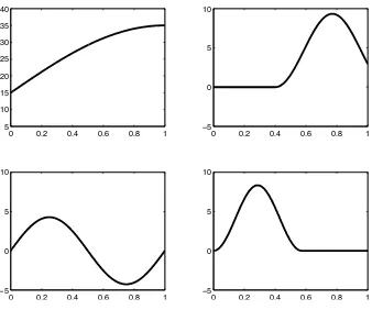
The nonzero coefficient functions used in all scenarios are displayed in Figure 2. The coefficient

functions do not belong to the B-spline function space.

In Scenario 1, we add a redundant variablex5(t) from normal distribution with mean zero and

0 0.2 0.4 0.6 0.8 1 5

10 15 20 25 30 35 40

0 0.2 0.4 0.6 0.8 1

−5 0 5 10

0 0.2 0.4 0.6 0.8 1

−5 0 5 10

0 0.2 0.4 0.6 0.8 1

−5 0 5 10

Figure 2: A graphical illustration of the coefficient functions βi i= 1, . . . ,4 (from left to right, top to

bottom)

with zero coefficient functions are defined asxi(t) =Zi(t) + 3/20

P5

l=1xl(t) fori= 6, . . . , pwithZi(t)’s

being iid from standard normal distribution.

The overall performance is measured in terms of bias and mean integrated squared error (MISE),

based onR= 400 repetitions, computed as

[

Biasi(u) = 1

R R X

r=1 b

βi(r)(u)−βi(u), i= 1, . . . , p, u∈[0,1],

\ M ISEi =

1

R R X

r=1 Z 1

0

(βb (r)

i (u)−βi(u))2du, i= 1, . . . , p,

whereβb

(r)

i is the estimated coefficient function from therth repeated study. In addition, we introduce

the following summary measures for comparison of functional sparsity:

(a) C0: average number of correctly identified constant zero coefficient functions

(c) Ci,0: average length of correctly identified zero intervals for the ith coefficient function

(d)Ii,0: average length of incorrectly identified zero intervals for theith coefficient function.

Note that (a) and (b) summarize global sparsity, while (c) and (d) summarize local sparsity.

Scenario 1: Effect of γ

Here, we consider the varying coefficient model with p = 5 and two different numbers of subjects

n = 100,200. In each iteration, our proposed PLSE method is implemented with γ = 0.25,0.35,0.5

and 0.75. The MISE values for every coefficient function are summarized in Table1. In general, as n

increases, all methods have smaller MISE values. Notably, the results for PLSE indicate comparable

performances across differentγ; in fact, PLSE and Lasso methods have similar performance in function

estimation. In addition, PLSE withγ = 0.35,0.50 can successfully identify the global sparsity ofβ5(·)

with zero MISE values for both choices of n, and so does PLSE with γ = 0.75 for n = 200. Bias of

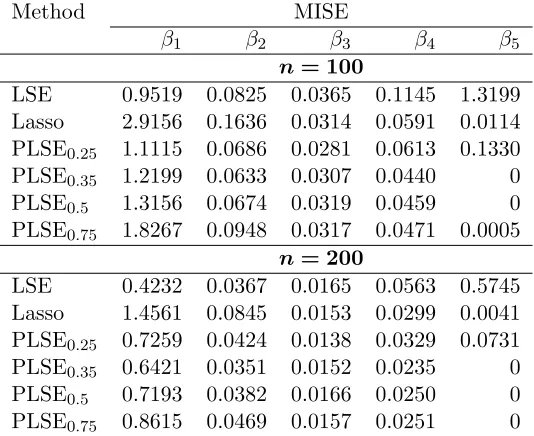
PLSE0.5 (PLSE withγ = 0.5), Lasso and LSE with n= 200 is compared in Figure 3. It can be seen

that PLSE0.5 has zero bias in estimating β5(·).

Method MISE

β1 β2 β3 β4 β5

n= 100

LSE 0.9519 0.0825 0.0365 0.1145 1.3199

Lasso 2.9156 0.1636 0.0314 0.0591 0.0114

PLSE0.25 1.1115 0.0686 0.0281 0.0613 0.1330

PLSE0.35 1.2199 0.0633 0.0307 0.0440 0

PLSE0.5 1.3156 0.0674 0.0319 0.0459 0

PLSE0.75 1.8267 0.0948 0.0317 0.0471 0.0005

n= 200

LSE 0.4232 0.0367 0.0165 0.0563 0.5745

Lasso 1.4561 0.0845 0.0153 0.0299 0.0041

PLSE0.25 0.7259 0.0424 0.0138 0.0329 0.0731

PLSE0.35 0.6421 0.0351 0.0152 0.0235 0

PLSE0.5 0.7193 0.0382 0.0166 0.0250 0

PLSE0.75 0.8615 0.0469 0.0157 0.0251 0

Table 1: Comparison of MISE for each coefficient function in Scenario 1.

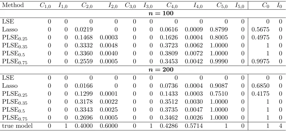
In Table 2, performance in identifying local sparsity is demonstrated. The true values of sparsity

in terms of Ci,0 and Ii,0 are given in the last row of true model as a reference. Hence, the closer the

0 0.2 0.4 0.6 0.8 1 -4

-2 0 2

0 0.2 0.4 0.6 0.8 1 -1

-0.5 0 0.5 1

0 0.2 0.4 0.6 0.8 1 -1

-0.5 0 0.5 1

0 0.2 0.4 0.6 0.8 1 -1

-0.5 0 0.5 1

0 0.2 0.4 0.6 0.8 1 -1

-0.5 0 0.5 1

Figure 3: Comparison of bias of the coefficient functions based on LSE (dot-dashed), Lasso (dashed)

and PLSE0.5 (solid) in Scenario 1 with n = 200. Note that PLSE0.5 has zero bias in estimating the

zero coefficient functionβ5(·).

model is the maximum error each method can make, so the smaller Ii,0, the better. In general, Lasso

and PLSE have better performance in functional sparsity. In addition, it can be seen that PLSE with

γ = 0.35,0.5,0.75 has an advantage in achieving both global and local sparsity compared with LSE

and Lasso. The case that γ = 0.5 slightly outperforms the others. For the remaining part, we will use

γ = 0.5 for comparison.

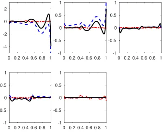
Scenario 2: Effect of dimension p

In this scenario, we study the effect of increasing p on the performance with a given sample size.

In particular, we consider three different choices of p = 5,20, and 50. Figure 4 and Table 3 show

the results of bias and MISE respectively. The last column of MISE tables indicates the maximum

MISE among the zero coefficient functions, as the selected variables vary between sample to sample.

Method C1,0 I1,0 C2,0 I2,0 C3,0 I3,0 C4,0 I4,0 C5,0 I5,0 C0 I0 n= 100

LSE 0 0 0 0 0 0 0 0 0 0 0 0

Lasso 0 0 0.0219 0 0 0 0.0616 0.0009 0.8799 0 0.5675 0

PLSE0.25 0 0 0.1468 0.0003 0 0 0.1626 0.0004 0.8005 0 0.4975 0

PLSE0.35 0 0 0.3332 0.0048 0 0 0.3723 0.0062 1.0000 0 1 0

PLSE0.5 0 0 0.3360 0.0040 0 0 0.3809 0.0072 1.0000 0 1 0

PLSE0.75 0 0 0.2559 0.0005 0 0 0.3453 0.0042 0.9990 0 0.9975 0

n= 200

LSE 0 0 0 0 0 0 0 0 0 0 0 0

Lasso 0 0 0.0166 0 0 0 0.0736 0.0004 0.9087 0 0.6850 0

PLSE0.25 0 0 0.1299 0.0001 0 0 0.1433 0.0003 0.7510 0 0.4175 0

PLSE0.35 0 0 0.3178 0.0022 0 0 0.3512 0.0030 1.0000 0 1 0

PLSE0.5 0 0 0.3343 0.0025 0 0 0.3735 0.0047 1.0000 0 1 0

PLSE0.75 0 0 0.2696 0.0005 0 0 0.3462 0.0026 1.0000 0 1 0

true model 0 1 0.4000 0.6000 0 1 0.4286 0.5714 1 0 1 4

Table 2: Sparsity summary measures (a)-(d) in Scenario 1. Here, for the true model,Ci,0,i= 1, . . . ,6

are the lengths of zero intervals, Ii,0’s are the lengths of nonezero intervals, C0 is the number of zero

coefficient functions, andI0 is the number of nonzero coefficient functions.

increasing dimension p.

Method MISE maxi≥6MISEi

β1 β2 β3 β4 β5

p= 5

LSE 0.4232 0.0367 0.0165 0.0563 0.5745 —

Lasso 1.4561 0.0845 0.0153 0.0299 0.0041 —

PLSE0.5 0.7193 0.0382 0.0166 0.0250 0 —

p= 20

LSE 0.5157 0.0434 0.0197 0.0612 0.6694 0.0151

Lasso 17.8758 0.8520 0.0331 0.0347 0 0.0016

PLSE0.5 0.7422 0.0391 0.0166 0.0240 0 2.1886e-05

p= 50

LSE 0.8269 0.0724 0.0292 0.0897 1.1484 0.0281

Lasso 35.1543 1.6475 0.0497 0.0415 0 8.4758e-04

PLSE0.5 0.7360 0.0396 0.0149 0.0205 0 2.7551e-05

Table 3: Comparison of MISE for each coefficient function with p= 5,20 and 50 in Scenario 2.

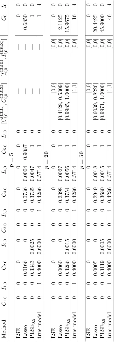
The performance of sparsity is summarized in Table 4. The additional two columns in Ci,0 and

Ii,0 are added to summarize the performance on all other redundant variables, as an interval range of

Metho

d

C1

,

0

I1,

0

C2

,

0

I2,

0

C3

,

0

I3,

0

C4

,

0

I4,

0

C5

,

0

I5,

0 0.5 1 -4

-2 0 2

0 0.5 1

-1 0 1

0 0.5 1

-1 0 1

0 0.5 1

-1 0 1

0 0.5 1

-4 -2 0 2

0 0.5 1

-1 0 1

0 0.5 1

-1 0 1

0 0.5 1

-1 0 1

0 0.5 1

-4 -2 0 2

0 0.5 1

-1 0 1

0 0.5 1

-1 0 1

0 0.5 1

-1 0 1

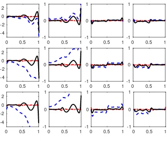
Figure 4: Comparison of bias of the nonzero coefficient functionsβ1, β2, β3 andβ4 (from left to right)

based on LSE (dot-dashed), Lasso (dashed) and PLSE0.5 (solid) for p= 5 (top row), p= 20 (middle)

and p= 50 (bottom) in Scenario 2.

andI0, we can conclude that PLSE0.5 systematically outperforms the other methods for all dimensions.

Scenario 3: Effect of knots selection

The variation in knots selection is expected to mainly influence the estimation of local sparsity.

In-creasing number of knots helps in identifying the boundary of local sparsity, with the risk of over-fitting

non-zero estimates. Fine-tuning this parameter is much more delicate, as all model selection criteria

are developed to control the squared error loss (MISE) as goodness of fit, and thus are insensitive to

the loss of missing local sparsity. That is, balance between global and local sparsity is beyond the usual

control of bias and variance trade-off, and developing a new measure is still an open problem. Our

knot selection based on cross-validation is essentially tuned towards global sparsity. Here we assess the

performance of our proposed estimator from the point of view of robustness to these variations. For

0 0.5 1 -4

-2 0 2

0 0.5 1

-1 -0.5 0 0.5 1

0 0.5 1

-1 -0.5 0 0.5 1

0 0.5 1

-1 -0.5 0 0.5 1

0 0.5 1

-4 -2 0 2

0 0.5 1

-1 -0.5 0 0.5 1

0 0.5 1

-1 -0.5 0 0.5 1

0 0.5 1

-1 -0.5 0 0.5 1

0 0.5 1

-4 -2 0 2

0 0.5 1

-1 0 1

0 0.5 1

-1 0 1

0 0.5 1

-1 0 1

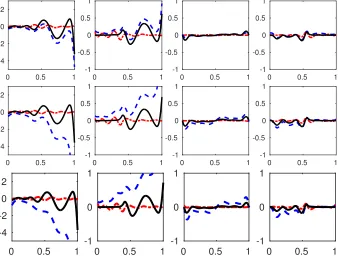
Figure 5: Comparison of bias of the nonzero coefficient functionsβ1, β2, β3 andβ4 (from left to right)

based on LSE (dot-dashed), Lasso (dashed) and PLSE0.5 (solid) for p= 5 (top row), p= 20 (middle)

Figure 5 and Table 5 summarize the bias and MISE. The sparsity summary is given in Table 6.

We conclude that the overall performance is fairly comparable to those in Scenario 2 with no major

concern over the sensitivity of the knots selection in comparison of the result.

Method MISE maxi≥6MISEi

β1 β2 β3 β4 β5

p= 5

LSE 0.2783 0.0253 0.0108 0.0379 0.3888 —

Lasso 1.2993 0.0753 0.0096 0.0195 0.0029 —

PLSE0.5 0.6888 0.0405 0.0107 0.0154 0 —

p= 20

LSE 0.3376 0.0292 0.0127 0.0408 0.4429 0.0097

Lasso 11.6604 0.5420 0.0199 0.0211 0 0.0011

PLSE0.5 0.7180 0.0412 0.0114 0.0156 0 2.1444e-05

p= 50

LSE 0.4521 0.0387 0.0167 0.0528 0.6608 0.0138

Lasso 30.2698 1.3683 0.0352 0.0290 0 7.0743e-04

PLSE0.5 0.7279 0.0417 0.0114 0.0150 0 1.9744e-05

Table 5: Comparison of MISE for each coefficient function in Scenario 3 . Here, the number of knots

is fixed to be 11.

In addition, in order to assess the usefulness of the asymptotic formula for the standard errors

in (2.6), both asymptotic and empirical standard errors based on 400 repetitions are calculated, and

compared in Figure6with adaptive number of knots and in Figure7with fixed number of knots, which

show a good agreement between them. It can be seen that the variation in number of knots greatly

increases the variation in estimation of coefficient functions.

In summary, the simulation results demonstrate that our proposed method not only has an

advan-tage in achieving local sparsity compared with Lasso and LSE, but also can ensure global sparsity for

finite dimensional models. Moreover, this advantage is carried onto models with increasing dimension.

5

Real Data Analysis

We demonstrate our method in an application to the analysis of yeast cell cycle gene expression data [14,

18].

In biological sciences, gene expression data are frequently collected. Scientists believe that

Metho

d

C1

,

0

I1,

0

C2

,

0

I2,

0

C3

,

0

I3,

0

C4

,

0

I4,

0

C5

,

0

I5,

0 0.5 1 0

1 2 3 4 5

0 0.5 1 0

0.1 0.2 0.3

0 0.5 1 0

0.01 0.02 0.03 0.04

0 0.5 1 0

0.02 0.04 0.06 0.08

0 0.5 1 0

1 2 3 4 5

0 0.5 1 0

0.1 0.2 0.3

0 0.5 1 0

0.01 0.02 0.03

0 0.5 1 0

0.02 0.04 0.06 0.08

0 0.5 1 0

1 2 3 4 5

0 0.5 1 0

0.1 0.2 0.3

0 0.5 1 0

0.01 0.02 0.03

0 0.5 1 0

0.02 0.04 0.06 0.08

Figure 6: Asymptotic standard error (grey solid line), and empirical standard deviation (black solid

0 0.5 1 0

5

0 0.5 1 0

0.1 0.2

0 0.5 1 0

0.02 0.04

0 0.5 1 0

0.02 0.04

0 0.5 1 0

5

0 0.5 1 0

0.1 0.2

0 0.5 1 0

0.02 0.04

0 0.5 1 0

0.02 0.04

0 0.5 1 0

5

0 0.5 1 0

0.1 0.2

0 0.5 1 0

0.02 0.04

0 0.5 1 0

0.02 0.04

Figure 7: Asymptotic standard error (grey solid line), and empirical standard deviation (black solid

in identifying key TFs in the regulatory network based on a set of gene expression measurements. In

this study, we analyze the relationship between the level of gene expression and the physical binding

of TFs from chromatin immunoprecipitation (ChIP-chip) data [14]. One of the gene expression data

comes from anα factor synchronization experiment of 542 genes, in which mRNA levels are measured

every 7 minutes during 119 minutes, resulting in 18 measurements in total [18]. For our analysis, the

time has been rescaled to [0,1].

0 0.5 1 -0.5

0

0.5 ACE2

0 0.5 1 -0.5

0

0.5 SWI4

0 0.5 1 -0.5

0

0.5 SWI5

0 0.5 1 -0.5

0

0.5 SWI6

0 0.5 1 -0.5

0

0.5 MBP1

0 0.5 1 -0.5

0

0.5 STB1

0 0.5 1 -0.5

0

0.5 FKH1

0 0.5 1 -0.5

0

0.5 FKH2

0 0.5 1 -0.5

0

0.5 NDD1

0 0.5 1 -0.5

0

0.5 MCM1

0 0.5 1 -0.5

0

0.5 ABF1

0 0.5 1 -0.5

0

0.5 BAS1

0 0.5 1 -0.5

0

0.5 CBF1

0 0.5 1 -0.5

0

0.5 GCN4

0 0.5 1 -0.5

0

0.5 GCR1

0 0.5 1 -0.5

0

0.5 GCR2

0 0.5 1 -0.5

0

0.5 LEU3

0 0.5 1 -0.5

0

0.5 MET31

0 0.5 1 -0.5

0

0.5 REB1

0 0.5 1 -0.5

0

0.5 SKN7

0 0.5 1 -0.5

0

0.5 STE12

Figure 8: Subplots of estimated coefficient functions for the 21 confirmed TFs using LSE (dashed),

Lasso (dot-dashed) and PLSE0.5 (solid).

The ChIP-chip data contains the binding information of 106 transcription factors, among which 21

TFs are confirmed to be related to cell cycle regulation by experiment. Wang et al. [23] demonstrated

that a variable selection procedure is able to identify some of those key TFs. It is believed that the

effects of TFs vary during the cell cycle. In [1], the authors considered a sparse partial least squares

regression to study which TFs are important in gene expression. But they did not focus on the active

periods of TFs. In this paper we apply our method to identify the key TFs and estimate the effects

of those selected TFs over time. In addition, our approach allows us to investigate whether active and

inactive periods during the cycle could be identified for each TF. Let ykt denote the gene expression

of transcription factorifor genek, fori= 1, . . . ,106. Then the varying coefficient model can be written

as

ykt=β0(t) + 106 X

i=1

βk(t)xik+kt,

where βi(t) models the effect of the ith transcription factor on gene expression at timet, and for the

k-th gene kt’s are independent over time.

Similar to the simulation study, we apply our method together with LSE and Lasso methods and

compared the identification of active period of each TF within the cell cycle process. Each coefficient

function is approximated with quadratic B-splines defined on time interval [0,1] with seven equally

spaced knots. The number of knots is selected by cross-validation. It is not surprising that LSE selects

all TFs. The lasso method identifies 32 TFs as important, while our proposed method identifies 16

TFs, which are in fact the subset of those identified by the lasso method. In Figure 8, the estimated

coefficient functions for 21 experimentally confirmed TFs are shown. From this figure, we could tell 8

of them are selected by both methods. The lasso method selects additional four TFs, namely, SWI4,

STB1, FKH1, REB1, which show very low level of activities. In [1], the authors selected 32 TFs, 10 of

which are verified TFs. In addition, our proposed method identifies some inactive periods for selected

TFs. For example, STE12 tends to be inactive for the later period, and ACE2 is inactive at early

period.

Acknowledgement

The authors are grateful to three referees and the associate editor for careful reading and helpful

comments, which have lead to substantial improvements of the paper. The research of Haonan Wang

was partially supported by NSF grants DMS-1106975, DMS-1521746 and DMS-1737795.

Supplementary Material

The online supplementary material includes technical assumptions and proofs of the theoretical

References

[1] Chun, H. and Kele¸s, S. (2010). Sparse partial least squares regression for simultaneous dimension

reduction and variable selection. Journal of the Royal Statistical Society: Series B, 72:3–25.

[2] de Boor, C. (2001). A Practical Guide to Splines. Springer.

[3] Diggle, P., Heagerty, P., Liang, K.-Y., and Zeger, S. (1994). Analysis of longitudinal data. OUP

Oxford.

[4] Hall, P. and Hooker, G. (2016). Truncated linear models for functional data. Journal of the Royal

Statistical Society: Series B (Statistical Methodology), 78(3):637–653.

[5] Hastie, T. and Tibshirani, R. (1993). Varying-coefficient models. Journal of the Royal Statistical

Society: Series B, 55:757–796.

[6] Hoover, D. R., Rice, J. A., Wu, C. O., and Yang, L. (1998). Nonparametric smoothing estimates

of time-varying coefficient models with longitudinal data. Biometrika, 85:809–822.

[7] Huang, J., Horowitz, J. L., and Wei, F. (2010). Variable selection in nonparametric additive models.

Annals of Statistics, 38(4):2282–2313.

[8] Huang, J., Ma, S., Xie, H., and Zhang, C.-H. (2009). A group bridge approach for variable selection.

Biometrika, 96:339–355.

[9] Huang, J. Z., Wu, C. O., and Zhou, L. (2002). Varying-coefficient models and basis function

approximations for the analysis of repeated measurements. Biometrika, 89:111–128.

[10] Huang, J. Z., Wu, C. O., and Zhou, L. (2004). Polynomial spline estimation and inference for

varying coefficient models with longitudinal data. Statistica Sinica, 14:763–788.

[11] James, G. M., Wang, J., and Zhu, J. (2009). Functional linear regression that’s interpretable.

Annals of Statistics, 37:2083–2108.

[12] Kneip, A., Poß, D., and Sarda, P. (2016). Functional linear regression with points of impact. Ann.

Statist., 44(1):1–30.

[13] Knight, K. and Fu, W. (2000). Asymptotics for lasso-type estimators. Annals of Statistics,

[14] Lee, T., Rinaldi, N., Robert, F., Odom, D., Bar-Joseph, Z., Gerber, G., Hannett, N., Harbison,

C., Thomson, C., Simon, I., Zeitlinger, J., Jennings, E., Murray, H., Gordon, D., Ren, B., Wyrick,

J., Tagne, J., Volkert, T., Fraenkel, E., Gifford, D., and Young, R. (2002). Transcriptional regulatory

networks in saccharomyces cerevisiae. Science, 298:799–804.

[15] M¨uller, H.-G. (2016). Peter hall, functional data analysis and random objects. Ann. Statist.,

44(5):1867–1887.

[16] Noh, H. S. and Park, B. U. (2010). Sparse varying coefficient models for longitudinal data.

Statistica Sinica, 20:1183–1202.

[17] Schumaker, L. (1981). Spline Functions: Basic Theory. Wiley.

[18] Spellman, P., Sherlock, G., Zhang, M., Iyer, V., Anders, K., Eisen, M., Brown, P., Botstein,

D., and Futcher, B. (1998). Comprehensive identification of cell cycle-regulated genes of the yeast

saccharomyces cerevisiae by microarray hybridization. Molecular Biology of the Cell, 9:3273–3279.

[19] Stone, C. J. (1982). Optimal global rates of convergence for nonparametric regression. The Annals

of Statistics, 10:1040–1053.

[20] Tu, C. Y., Song, D., Breidt, F. J., Berger, T. W., and Wang, H. (2012). Functional model

selection for sparse binary time series with multiple input. In Economic Time Series: Modeling and

Seasonality, pages 477–497. Chapman and Hall/CRC.

[21] Wahba, G. (1990). Spline Models for Observational Data. CBMS-NSF Regional Conference Series

in Applied Mathematics. Society for Industrial and Applied Mathematics.

[22] Wang, H. and Kai, B. (2015). Functional sparsity: Global versus local. Statistica Sinica, 25:1337–

1354.

[23] Wang, L., Chen, G., and Li, H. (2007). Group scad regression analysis for microarray time course

gene expression data. Bioinformatics, 23:1486–1494.

[24] Wang, L., Li, H., and Huang, J. Z. (2008). Variable selection in nonparametric varying-coefficient

models for analysis of repeated measurements. Journal of the American Statistical Association,

103:1556–1569.

[25] Wei, F., Huang, J., and Li, H. (2011). Variable selection and estimation in high-dimensional

[26] Wu, H. and Zhang, J.-T. (2006). Nonparametric regression methods for longitudinal data analysis:

mixed-effects modelling approaches. Wiley.

[27] Xue, L. and Qu, A. (2012). Variable selection in high-dimensional varying-coefficient models with

global optimality. The Journal of Machine Learning Research, 13:1973–1998.

[28] Yao, F., M¨uller, H.-G., and Wang, J.-L. (2005). Functional data analysis for sparse longitudinal

data. Journal of the American Statistical Association, 100:577–590.

[29] Zhao, P. and Yu, B. (2006). On model selection consistency of lasso. Journal of Machine Learning

Research, 7:2541–2563.

[30] Zhou, J., Wang, N.-Y., and Wang, N. (2013). Functional linear model with zero-value coefficient