http://www.scirp.org/journal/jamp ISSN Online: 2327-4379 ISSN Print: 2327-4352
DOI: 10.4236/jamp.2018.61024 Jan. 29, 2018 247 Journal of Applied Mathematics and Physics
Some Features of Neural Networks as
Nonlinearly Parameterized Models of Unknown
Systems Using an Online Learning Algorithm
Leonid S. Zhiteckii
1, Valerii N. Azarskov
2, Sergey A. Nikolaienko
1, Klaudia Yu. Solovchuk
11Department of Intelligent Automatic Systems, International Centre of Information Technologies and Systems, Institute of Cybernetics, Kiev, Ukraine
2Aircraft Control Systems Department, National Aviation University, Kiev, Ukraine
Abstract
This paper deals with deriving the properties of updated neural network mod-el that is exploited to identify an unknown nonlinear system via the standard gradient learning algorithm. The convergence of this algorithm for online training the three-layer neural networks in stochastic environment is studied. A special case where an unknown nonlinearity can exactly be approximated by some neural network with a nonlinear activation function for its output layer is considered. To analyze the asymptotic behavior of the learning processes, the so-called Lyapunov-like approach is utilized. As the Lyapunov function, the expected value of the square of approximation error depending on network parameters is chosen. Within this approach, sufficient conditions guaranteeing the convergence of learning algorithm with probability 1 are de-rived. Simulation results are presented to support the theoretical analysis.
Keywords
Neural Network, Nonlinear Model, Online Learning Algorithm, Lyapunov Function, Probabilistic Convergence
1. Introduction
Design of mathematical models for technical, economic, social and other sys-tems with uncertainties is the important problem from both theoretical and practical points of view. This problem attracts close attention of many researches. The significant progress in this scientific area has been achieved last time. Within this area, new methods and modern intelligent algorithms dealing with uncertain How to cite this paper: Zhiteckii, L.S.,
Azarskov, V.N., Nikolaienko, S.A. and So-lovchuk, K.Yu. (2018) Some Features of Neural Networks as Nonlinearly Paramete-rized Models of Unknown Systems Using an Online Learning Algorithm. Journal of Applied Mathematics and Physics, 6, 247-263.
https://doi.org/10.4236/jamp.2018.61024
Received: October 31, 2017 Accepted: January 26, 2018 Published: January 29, 2018
Copyright © 2018 by authors and Scientific Research Publishing Inc. This work is licensed under the Creative Commons Attribution International License (CC BY 4.0).
http://creativecommons.org/licenses/by/4.0/
DOI: 10.4236/jamp.2018.61024 248 Journal of Applied Mathematics and Physics systems have recently been proposed in [1][2][3][4]. They include some new optimization approaches advanced, in particular, in the papers [2][4].
Over the past decades, interest has been increasing toward the use multilayer neural networks applied among other as models for the adaptive identification of nonlinearly parameterized dynamic systems [5][6][7][8]. This has been moti-vated by the theoretical works of several researches [9] [10] who proved that, even with one hidden layer, neural network can uniformly approximate any continuous mapping over a compact domain, provided that the network has suf-ficient number of neurons with corresponding weights. The theoretical back-ground on neural network modeling may be found in the book [11].
Different learning methods for updating the weights of neural networks have been reported in literature. Most of these methods rely on the gradient concept [8]. One of these methods is based on utilizing the Lyapunov stability theory [6] [12].
The convergence of the online gradient training procedure dealing with input signals that have deterministic (non-stochastic) nature was studied by many au-thors [13]-[23]. Several of these authors assumed that training set must be finite whereas in online identification schemes, this set is theoretically infinite. Never-theless, recently we observed a non-stochastic learning process when this pro-cedure did not converge for certain infinite sequence of training examples [24].
The probabilistic asymptotic analysis on convergence of the online gradient training algorithms has been conducted in [25]-[33]. Several of their results make it possible to employ a constant learning rate [28][30]. To the best of au-thor’s knowledge, there are no general results in literature concerning the global convergence properties of training procedures with a fixed learning rate applica-ble to the case of infinite learning set.
A popular approach to analyze the asymptotic behavior of online gradient al-gorithms in stochastic case is based on Martingale convergence theory [34]. This approach has been exploited by the authors in [24] to derive some local conver-gence in stochastic framework for standard online gradient algorithms with the constant learning rate.
The difficulties associated with convergence properties of online gradient learning algorithms are how to guarantee the boundedness of the network weights biases assuming the learning process to be theoretically infinite. To overcome these difficulties, the penalty term to an error function has been in-troduced in [33]. Recently we however established in [35] that the global con-vergence of these algorithms with probability 1 can be achieved without any ad-ditional term, at least, in the case when the activation function of the network output layer is linear.
DOI: 10.4236/jamp.2018.61024 249 Journal of Applied Mathematics and Physics constant? As pointed out in [23], the answer to the question on convergence properties of this standard algorithm which should shed some light on asymp-totic features of multilayer neural networks using the gradient-like training technique is the first step toward a full understanding of other more generic training algorithms based on regularization, conjugate gradient, and Newton optimization methods, etc.
Novelty of this paper which extends the basic ideas of [35] to the case where the activation function of the output layer is nonlinear, consists in establishing sufficient conditions under which the gradient algorithm for learning neural networks will globally converge in the sense almost sure for the case when the learning rate can be constant. The proposed approach to deriving these conver-gence results is based on utilizing the Lyapunov methodology [36]. They make it possible to reveal some new features of the multilayer neural networks with non-linear activation function in output layer which use the online gradient-type training algorithms having a constant learning rate.
2. Description of Learning Neural Network System: Problem
Formulation
Consider the typical three-layer feedforward neural network containing a hidden layer and p inputs, q hidden neurons, and one output neuron. Denote by
( )
T1, ,
ij q p q
W= w × = w w
with
T
1, , , 1, ,
p
i i ip
w =w w ∈R i= q
the weight matrix connecting the input and hidden layers, and define the so-called bias vector w0 as
T
0 01, , 0 ,
q q
w =w w ∈R
which is the threshold in the hidden-layer output. Further, let
T
1, , ,
q q
ω=ω ω ∈R
be the weight vector between the hidden and output layers, and ω0 be the bias
in the output layer. As in [33], the activation functions used in the hidden neu-rons are all the same denoted by g:R→R, and the activation function for the output layer is f:R→R.
Now, denoting by
( )
( )
( )
T1 , , q
G z = g z g z
the vector-valued function which depends on the vector T 1, ,
q q
z=z z ∈R , introduce the extended matrix
[
]
( 1)0
q p
W = W w ∈R× + by adding the column w0 to W and the extended vector T T 1
0
, q
ω=ω ω ∈ +
R , and also the function
( )
( )
( )
T1 , , q ,1
G z = g z g z of z. Then the for an input vector
T
1, , ,
p p
DOI: 10.4236/jamp.2018.61024 250 Journal of Applied Mathematics and Physics the output vector of hidden layer can be written as G W x
( )
, where the notationT T
,1
x= x of the extended vector x∈Rp+1 is used, and the final output
NN
y ∈R of the neural network can be expressed as follows:
( )
(
T)
NN .
y = f ω G Wx (1)
Let
( )
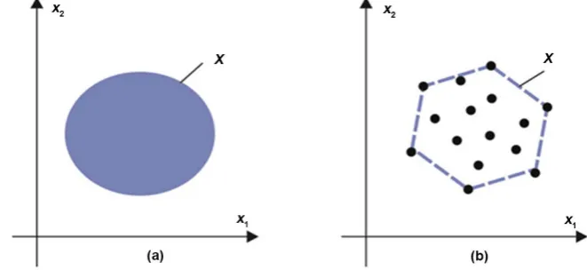
y=ϕ x (2) with ϕ:Rp →R be an unknown and bounded nonlinearity given over the bounded either finite or infinite sets X ⊂Rp which are depicted in Figure 1 for the case p=2. This function needs to be approximated by the neural
net-work (1) via suitable choice of ω and W . By virtue of (2) the approximation error
(
)
(
T( )
)
, , ,
e ωW x y = −y f ω G Wx (3)
depends on x for any fixed
(
ω,W)
.Now, suppose that some complex system to be identified is described at each nth time instant by the equation
( )
(
0,1, 2,)
n n
y =ϕ x n= (4) in which n
x ∈X and yn∈R are its input and output signals, respectively available for measurement.
Based on the infinite sequence of the training examples
{
n, n}
0 nx y ∞
= that is
generated by (4), the outline learning algorithm for updating the weight and bi-ases in (1) is defined as the standard gradient-descent iteration procedure
(
)
1 2
, ; , ,
n n n n n n
n ωe W y x ω + =ω − ∇η ω
(5)
(
)
1 2
, ; , ,
i
n n n n n n
i i n w
w+ =w − ∇η e ω W y x (6)
1, , , 0,1, .
i= q n=
In these equations, 2
(
)
, ; ,
e
ω
∇ ⋅ ⋅ ⋅ ⋅ and 2
(
)
, ; ,
i
we
∇ ⋅ ⋅ ⋅ ⋅ denote the current
gra-dients of the error function e2
(
ω,W y x; ,)
with respect to ω andi
[image:4.595.204.535.554.706.2]w,
DOI: 10.4236/jamp.2018.61024 251 Journal of Applied Mathematics and Physics respectively, obtained after substituting ω ω= n, n
W =W , y=yn, and n
x =x into (3), and η >n 0 represents the step size (the learning rate). Note that the expressions of 2
(
)
, ; ,
n n n n
e W y x
ω ω
∇ and 2
(
)
, ; ,
i
n n n n
we ω W y x
∇ may be writ-ten in detail similar to that in [23] [33]. (Due to space limitation, they are here omitted.)
Introducing the notation
T
T T T T
1 0
,w, ,w wq, θ= ω
of the extended weight and bias vector θ∈ q p( +1)
R , and considering the Equa-tions (5) and (6) in conjunction, rewrite the online gradient learning algorithm for updating θn in a general form (as in [33])
(
)
1 2 ; , ,
n n n n n
n θe y x
θ + =θ − ∇η θ (7) where 2
( )
; ,
e
θ
∇ ⋅ ⋅ ⋅ represents the gradient of e2
(
θn;y xn,n)
with respect toθ
calculated at the nth time instant.Thus, the Equation (7) together with the expression
(
; ,)
NN n n n n ne θ y x =y −y in which n
y is given by (4), and
(
)
NN ,
n n n
y =ψ θ x
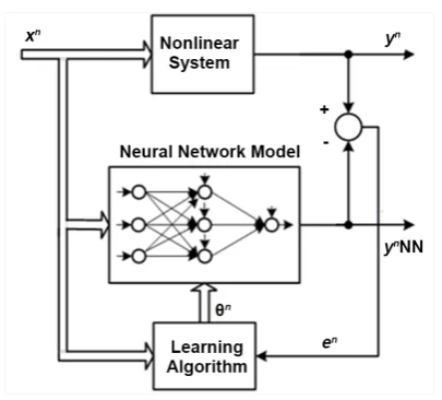
describe the learning neural network system necessary to identify the nonlinear-ity (2). For better understanding the performance of this system, its structure is depicted in Figure 2, where the notation en=e
(
θn;y xn, n)
is used.The problem formulated in this paper consists in analyzing asymptotic prop-erties of the learning neural network system presented above. More certainly, it is required to derive conditions under which the learning procedure will be convergent meaning the existence of a limit
lim n
n θ θ
∞
→∞ = (8)
in some sense [24].
3. Preliminaries
Suppose that there is a multilayer neural network described by
( )
NN , ,
y ≡ψ θ x
where
θ
is some fixed parameter vector. According to [9] [10], the require-ment( )
( )
max ,
x X∈ ϕ x −ψ θ x ≤ε
DOI: 10.4236/jamp.2018.61024 252 Journal of Applied Mathematics and Physics
Figure 2. Configuration of learning neural network system.
( )
( )
( )
0
max , .
x X
J θ ϕ x ψ θ x
∈
= − (9)
In fact, the desired (optimal) vector * 0
θ θ= will then be specified from (9) as the variable
θ
minimizing 0( )
J θ :
( )
( )
*
0 arg min max , .
x X x x
θ
θ ϕ ψ θ
∈
= − (10)
Nevertheless, all researches which employ online learning procedures in sto-chastic environment “silently” replace J0
( )
θ by( )
{
2(
)
}
; , ,
x
J θ =E e θ y x
where
{
2(
)
}
; , x
E e θ y x denotes the expected value of e2
(
θ; ,y x)
.Indeed, the learning algorithm (7) does not minimize (9): namely, it minimiz-es J
( )
θ (instead of J0( )
θ ) [37]. This observation means that (7) will at best yield( )
*: arg minJ .
θ
θ = θ
but not * 0
θ given by (10) as n→ ∞.
Now, consider a special case when the unknown function (2) can exactly be approximated by the neural network ψ θ
( )
,x implying( )
( )
*, .
x x x X
ϕ ≡ψ θ ∀ ∈ (11) In this case called in ([8], p. 304) by the ideal case, we have
( )
*, 0
eθ x ≡ for any x from X and, consequently, J
( )
θ* =0.If the condition given in identity (11) is satisfied, then the learning rate ηn in
(7) may be constant:
const 0;
n
η ≡ =η > see ([37], sect. 3.13).
Note that the property (11) may take place, in particular, when
( ) ( )
{
1}
, , K
DOI: 10.4236/jamp.2018.61024 253 Journal of Applied Mathematics and Physics provided that their number does not exceed the dimension of
θ
. To understand this fact, according to (11) write the set of K equations( )
(
)
( ) ( )(
)
( ) 1 1 ,, K K
x y x y ψ θ ψ θ = =
with respect to the unknown
θ
. They are compatible if K≤q p(
+2)
+1. Due to (2) together with the definition of θ* it can be concluded that their solutionis just θ θ= * yielding
( )
* 0J θ = because in this special case,
( )
(
*)
( ),xk yk
ψ θ = for all k=1,,K.
4. Main Results
4.1. Some Feature of Multilayer Neural Network
It turns out that if the activation functions g of the hidden layer are nonlinear, then for an arbitrary fixed vector θ′ there is, at least, one vector θ′′ such that
the network outputs for these different vectors are the same even though the output activation function f is linear, i.e. if f
( )
ζ =ζ :(
,x)
(
,x)
x X.ψ θ′ ≡ψ θ′′ ∀ ∈ (12)
The feature (12) gives that in the presence of nonlinear g there exist, at least, two different *
s
θ . For example, let p=1,q=1 and
( )
1( )
1 1 1 exp g z z = + −
in which z1=w x11 1+w01 , and f
( )
ζ =ζ with ζ ω= 1g z( )
1 +ω0 . Fix a[
]
T11, 01, 1, 0
w w
θ′= ′ ′ ω ω′ ′ . Then
[
]
T11, 01, 1, 1 0
w w
θ′′= − ′ − ′ −ω ω ω′ ′+ ′ will also satisfy (12);
see [35]. Therefore, the set of * s
θ will be not one-point if g is nonlinear.
4.2. An Observation
To study some asymptotic properties of sequence
{ }
θn caused by the learning algorithm (7) in the non-stochastic case, simulation experiments with the scalar nonlinear system (2) having the nonlinearity( )
3.75 0.05 exp(
(
7.15)
)
1 0.19 exp 7.15x x
x
ϕ = + −
+ −
were conducted. This nonlinearity can explicitly be approximated by the two-layer neural network model described by
( )
*,x
ψ θ as in Subsection 4.1
with ( )1
[
]
T7.15,1.65, 3.45, 0.3
θ∗ = and ( )2
[
]
T7.15, 1.65, 3.45, 3.75
θ∗ = − − − .
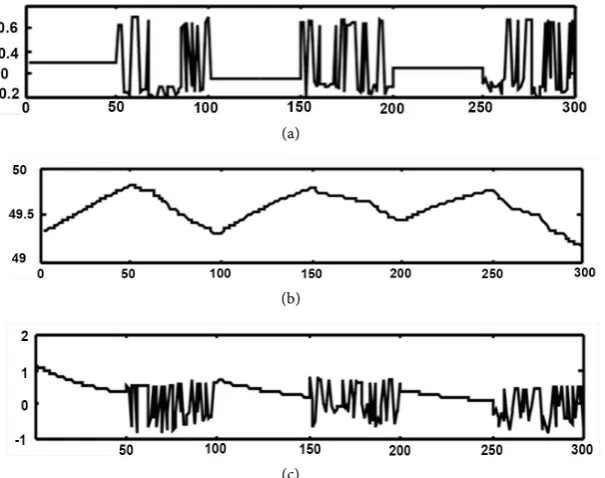
Figure 3 illustrates the results of the one simulation experiment with
0.01
η= , where
{ }
xn was chosen as a non-stochastic sequence. It can be ob-served that in this example, the variable *( )1,2
mini= θ i −θn shown in Figure
DOI: 10.4236/jamp.2018.61024 254 Journal of Applied Mathematics and Physics
(a)
(b)
[image:8.595.227.530.72.311.2](c)
Figure 3. Behaviour of learning algorithm (7) in non-stochastic case: (a) inputs n
e ; (b) the variable min
{
θ* 1( )−θn ,θ* 2( )−θn}
; (c) current model error en.4.3. Sufficient Conditions for the Probabilistic Convergence of
Learning Procedure
The following basic assumption concerning
{ }
n 0 nx ∞
= which is bounded
stochas-tic sequence (since X is bounded) is made:
(A1) xns arise randomly in accordance with a probability distribution
( )
P x if X is finite, and with probability density p x
( )
if X is infinite. Within assumption (A1), the expected value (mean) of(
)
(
( )
)
22
; , ,
e θ y x = y−ψ θ x is given by
(
)
{
}
(
) ( )
(
) ( )
2
2
2
; , if is finite set, ; ,
; , d if is infinite set.
x X x
X
e y x P x X
E e y x
e y x p x x X
θ θ
θ
∈ =
∑
∫
To derive the main theoretical result we need Assumption (A1) and the fol-lowing additional assumptions:
(A2) the identity (11) holds;
(A3) the activation functions used in the hidden neurons and output neuron are the same
(
f( )
⋅ =g( )
⋅)
, twice continuously differentiable onR
and also uniformly bounded onR
.Further, we introduce a scalar function V
( )
θ playing a role of the Lyapunov function [36] with the features:(a) V
( )
θ is nonnegative, i.e.,( )
0;V θ ≥ (13)
DOI: 10.4236/jamp.2018.61024 255 Journal of Applied Mathematics and Physics
( )
( )
V θ′ V θ′′ Lθ θ′ ′′
∇ − ∇ ≤ − (14)
for any θ θ′ ′′, from Rq p( +1), where ∇V
( )
θ denotes its gradient, and L>0 represents the Lipschitz constant.Now, the global stochastic convergence analysis of the gradient learning algo-rithm (7) is based on employing the fundamental convergence conditions estab-lished in the following Key Technical Lemma which is the slightly reformulated Theorem 3 of [36].
Key Technical Lemma. Let V
( )
θ be a function satisfying (13) and (14). Define the scalar variable( )
( )
T{
( )
}
,
H
θ
= ∇θVθ
∇θE Q xθ
(16) with some Q x( )
,θ ≥0, and denote( )
( )
T{
(
)
}
: n , n .
n
H θ = ∇θV θ ∇θE Q xθ
Suppose:
1)
( )
( )
1, 0,
n
n n n
H θ ≥ ΘV θ − Θ >
2) E
{
∇θQ x(
,θn)
2}
≤τnV( )
θn ,τn≥0. Introduce the additional variable(
2 .)
n n n L n n
ν =η Θ − η τ (17)
Then the algorithm (7) yields
lim n 0
n→∞V = a.s.,
where Vn:=V
( )
θn provided that E{ }
θ0 < ∞ and0≤νn≤1, (18)
0 .
n n
v
∞
=
= ∞
∑
(19)Related results followed from the Theorem 3’ of [36] are:
Corollary. Under the conditions of the Key Technical Lemma, if const
n
Θ ≡ Θ = and τn≡ =τ const, and ηn ≡ =η const, then Vnn→∞→0
with probability 1 provided that
(
)
(
)
0< ≤ Θ −η 2 ε Lτ 0< < Θε (20) is satisfied.
Next, we are able to present the convergence result summarized in the theo-rem below.
Theorem. Suppose Assumption (A2) holds. Then the gradient algorithm (7) with a constant learning rate, ηn≡η, will converge with probability 1 (in the
sense that Vnn→∞→0 a.s.) and
(
)
lim n; n, n 0
n→∞e θ y x = a.s. (21)
for any initial θ0 chosen randomly so that
{
(
0)
}
,DOI: 10.4236/jamp.2018.61024 256 Journal of Applied Mathematics and Physics
( )
{
}
( )
{
}
2 ,: inf 0,
, E Q x
E Q x
θ θ
θ θ ∇
Θ = > (22)
(
)
{
}
(
)
{
}
2 ,: sup .
,
E Q x
E Q x
θ θ θ τ θ ∇
= < ∞ (23)
Proof. Set V
( )
θ =E Q x{
( )
,θ}
. Then condition (13) and (14) can be shownto be valid. This indicates that this function may be taken as the Lyapunov func-tion. By virtue of (16) such a choice of V
( )
θ gives H( )
θ = ∇θE Q x{
( )
,θ}
2.Putting Θ ≡ Θn and τn≡τ with Θ and
τ
determined by (22) and (23),respectively, we can conclude that the conditions 1), 2) of the Key Technical Lemma are satisfied. Applying its Corollary it proves that limn→∞Vn=0 with probability 1.
Due to the fact that
( )
{
2(
)
}
; ,
x
V θ =E e θ y x together with Assumption (A2), result (21) follows.
4.4. Simulations and a Discussion
To demonstrate theoretical result given in Subsection 4.3, several simulations were conducted. First, we dealt with the same neural network and the same training samples as in ([33], p. 1052). Namely, they were chosen as follows:
( )1
[ ]
T ( )10, 0 , 1;
x = y =
( )2
[ ]
T ( )20,1 , 0;
x = y =
( )3
[ ]
T ( )31, 0 , 0;
x = y =
( )4
[ ]
T ( )41,1 , 1.
x = y =
The two numerical examples with different initial θ0 were considered. In
Example 1 we set 0
11 0.95
w = , w120 = −0.084 , 0
21 0.079
w = , w022= −0.079 , 0
01 0.089
w = − , 0
02 0.075
w = , 0
1 0.357
ω = , 0
2 0.357
ω = − , 0
0 0.354
ω = . In Example 2 we set 0
11 0.090
w = − , w120 =0.225, 0
21 0.138
w = − , w220 =0.139, 0
01 0.222
w = ,
0
02 0.084
w = − , 0
1 0.356
ω = − , 0
2 0.357
ω = , 0
0 0.353
ω = .
Contrary to [33] the learning rate was chosen as η=0.01 in order to
imple-ment the algorithms (5), (6) with no penalty term.
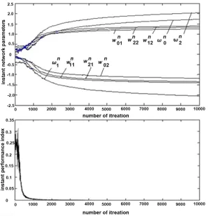
Results of two simulation experiments whose durations were 10000 iteration steps are presented in Figure 4 and Figure 5 in which the components of θn
and
( )
nJ θ are shown.
Further, another simulation experiments were also conducted. In contrast with previous experiments, they dealt with an infinite training sets X Namely, the two simulations with the same nonlinear function as in Subsection 4.2 were first conducted, provided that X is the infinite bounded set given by X∈ −
[
2, 2]
. However,{ }
nx was now chosen as the stochastic sequence. Namely, it was generated as a pseudorandom i.i.d. sequence.
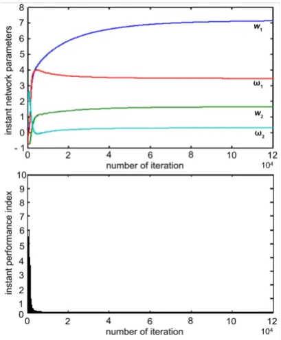
Two numerical examples were considered. In Example 3, the initial values of neural network weights and biases were taken as follows: 0
1 0.529
DOI: 10.4236/jamp.2018.61024 257 Journal of Applied Mathematics and Physics
Figure 4. Behavior of gradient learning algorithm (7) in Example 1.
[image:11.595.225.525.395.707.2]DOI: 10.4236/jamp.2018.61024 258 Journal of Applied Mathematics and Physics 0
2 0.5012
w = − , ω = −10 0.9168 , 0
2 1.0409
ω = . In Example 4 we set
0
1 0.3756
w = − , w20= −0.572, 0
1 0.9798
ω = − , 0
2 1.1436
ω = . Figure 6 and Figure 7 demonstrate results of the two simulation experiments conducted with the ini-tial estimates θ0 given above. In both experiments,
n
η was also chosen as 0.01
n
η ≡ =η .
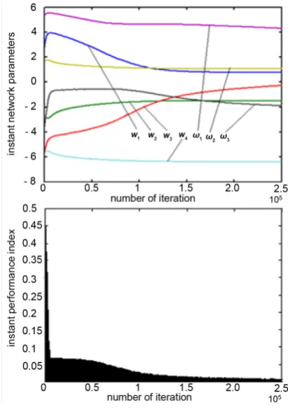
Next, another nonlinearity
( )
( )
( )
1 2
1
1 exp 1
x
a x a x
ϕ =
+ − − −
with
( )
(
)
11 1 exp 10 5
a x = + − x− − and a2
( )
x 1 exp(
10x 5)
1 −= + − + to be exactly approximated by a suitable neural network was chosen as in [11, p. 12-4]. The following initial estimates were taken: 0
1 2.8
w = , 0
2 5.6
w = − , 0
3 2.8
w = − ,
0
4 5.6
w = − , ω =10 5.33, 0
2 1.71
ω = , 0
3 3.52
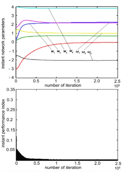
ω = − (Example 5), and 0
1 0.27
w = ,
0
2 0.19
w = , 0
3 3.09
w = − , 0
4 3.96
w = , 0
1 1.64
ω = , 0
2 0.72
ω = , 0
3 2.21
ω = − (Ex-ample 6).
Results of the two simulation experiments conducted with the initial estimates
0
θ given above are depicted in Figure 8 and Figure 9.
From Figures 4-9 we can see that the learning processes converge and the performance index J
( )
θn tends to zero while the penalty term is absent. It can be observed that if the initial vectors 0s
θ are different then the sequences
{ }
θn may converge to different finals θ∞ .
[image:12.595.271.476.448.696.2]The simulation experiments show that the penalty term is not necessary, in principle, to achieve the convergence of the online gradient learning procedure in the three-layer neural networks if certain conditions given by Assumption (A1)-(A3) are satisfied. This fact supports our theoretical results.
DOI: 10.4236/jamp.2018.61024 259 Journal of Applied Mathematics and Physics
Figure 7. Behavior of gradient learning algorithm (7) in Example 4.
[image:13.595.274.480.402.696.2]DOI: 10.4236/jamp.2018.61024 260 Journal of Applied Mathematics and Physics
Figure 9. Behavior of gradient learning algorithm (7) in Example 6.
5. Conclusion
In this paper, some important features of multilayer neural networks which are utilized as nonlinearly parameterized models of unknown nonlinear systems to be identified have been derived. A special case where the nonlinearity can exactly be approximated by a three-layer neural network has been studied. Contrary to previous author’s papers we dealt with the neural network having a nonlinear activation function for its output layer. It was shown that if the activation func-tion of the hidden layer is nonlinear, then, for any input variables, there are, at least, two different network parameter vectors under which the network outputs will be the same even though the output activation function is linear. This fea-ture gives that the standard gradient online training algorithm with a constant learning rate may not be convergent if the training sequence is non-stochastic. Nevertheless, provided that this sequence is stochastic, it has theoretically been established that, under certain conditions, such algorithm will converge with probability one. However, ultimate values of network parameters may be differ-ent. These facts were confirmed by simulation experiments.
Acknowledgements
The authors are grateful to anonymous reviewer for his valuable comments.
References
DOI: 10.4236/jamp.2018.61024 261 Journal of Applied Mathematics and Physics Selection Based on Uncertain Semivariance. International Journal of Systems Science, 3, 637-648. https://doi.org/10.1080/00207721.2016.1206985
[2] Draa, A., Bouzoubia, S. and Boukhalfa, I. (2015) A Sinusoidal Differential Evolution Algorithm for Numerical Optimisation. Applied Soft Computing, 27, 99-126.
https://doi.org/10.1016/j.asoc.2014.11.003
[3] Zhang, B., Peng, J., Li, S. and Chen, L. (2016) Fixed Charge Solid Transportation Problem in Uncertain Environment and Its Algorithm. Computers & Industrial En-gineering, 102, 186-197. https://doi.org/10.1016/j.cie.2016.10.030
[4] Sun, G., Zhao, R. and Lan, Y. (2016) Joint Operations Algorithm for Large-Scale Global Optimization. Applied Soft Computing, 38, 1025-1039.
https://doi.org/10.1016/j.asoc.2015.10.047
[5] Suykens, J. and Moor, B.D. (1993) Nonlinear System Identification Using Multilay-er Neural Networks: Some Ideas for Initial Weights, NumbMultilay-er of Hidden Neurons and Error Criteria. Proceedings of the 12th IFAC World Congress, Sydney, Aus-tralia, 3, 49-52.
[6] Kosmatopoulos, E.S., Polycarpou, M.M., Christodoulou, M.A. and Ioannou, P.A. (1995) High-Order Neural Network Structures for Identification of Dynamical Sys-tems. IEEE Transactions on Neural Networks, 6, 422-431.
https://doi.org/10.1109/72.363477
[7] Levin, A.U. and Narendra, K.S. (1995) Recursive Identification Using Feedforward Neural Networks. International Journal of Control, 61, 533-547.
https://doi.org/10.1080/00207179508921916
[8] Tsypkin, Ya.Z., Mason, J.D., Avedyan, E.D., Warwick, K. and Levin, I.K. (1999) Neural Networks for Identification of Nonlinear Systems Under Random Piecewise Polynomial Disturbances. IEEE Transactions on Neural Networks, 10, 303-311.
https://doi.org/10.1109/72.750559
[9] Cybenko, G. (1989) Approximation by Superpositions of a Sigmoidal Functions. Mathematics of Control, Signals, and Systems, 2, 303-313.
[10] Funahashi, K. (1989) On the Approximate Realization of Continuous Mappings by Neural Networks. Neural Networks, 2, 182-192.
https://doi.org/10.1016/0893-6080(89)90003-8
[11] Hagan, M.T., Demuth, H.B. and Beale, M.H. (1996) Neural Network Design. PWS Publishing, Boston.
[12] Behera, L., Kumar, S. and Patnaik, A. (2006) On Adaptive Learning Rate That Guarantees Convergence in Feedforward Networks. IEEE Transactions on Neural Networks, 17, 1116-1125.https://doi.org/10.1109/TNN.2006.878121
[13] Mangasarian, O.L. and Solodov, M.V. (1994) Serial and Parallel Backpropagation Convergence via Nonmonotone Perturbed Minimization. Optimization Methods of Software, 4, 103-116, 199.https://doi.org/10.1080/10556789408805581
[14] Luo, Z. and Tseng, P. (1994) Analysis of an Approximate Gradient Projection Me-thod with Application to the Backpropagation Algorithm. Optimization Methods of Software, 4, 85-101.https://doi.org/10.1080/10556789408805580
[15] Ellacott, S.W. (1993) The Numerical Analysis Approach. In: Taylor, J.G., Ed., Ma-thematical Approaches to Neural Networks, Elsevier Science Publisher B.V., Ams-terdam, 103-137.https://doi.org/10.1016/S0924-6509(08)70036-9
DOI: 10.4236/jamp.2018.61024 262 Journal of Applied Mathematics and Physics [17] Wu, W. and Xu, Y.S. (2002) Deterministic Convergence of an Online Gradient Me-thod for Neural Networks. Journal of Computational and Applied Mathematics, 144, 335-347.https://doi.org/10.1016/S0377-0427(01)00571-4
[18] Wu, W., Feng, G.R., Li, X. and Xu, Y.S. (2005) Deterministic Convergence of an Online Gradient Method for BP Neural Networks. IEEE Transactions on Neural Networks, 16, 1-9.https://doi.org/10.1109/TNN.2005.844903
[19] Wu, W., Feng, G. and Li, X. (2002) Training Multilayer Perceptrons via Minimiza-tion of Ridge FuncMinimiza-tions. Advances in Computational Mathematics, 17, 331-347.
https://doi.org/10.1023/A:1016249727555
[20] Wu, W., Shao, H. and Qu, D. (2005) Strong Convergence for Gradient Methods for BP Networks Training. Proceedings of 2005 International Conference on Neural Networks and Brain, Beijing, 13-15 October 2005, 332-334.
https://doi.org/10.1109/ICNNB.2005.1614626
[21] Zhang, N., Wu, W. and Zheng, G. (2006) Convergence of Gradient Method with Momentum for Two-Layer Feedforward Neural Networks. IEEE Transactions on Neural Networks, 17, 522-525.https://doi.org/10.1109/TNN.2005.863460
[22] Shao, H., Wu, W. and Liu, L. (2007) Convergence and Monotonicity of an Online Gradient Method with Penalty for Neural Networks. WSEAS Transactions on Ma-thematics, 6, 469-476.
[23] Xu, Z.B., Zhang, R. and Jing, W.-F. (2009) When Does Online BP Training Con-verge? IEEE Transactions on Neural Networks, 20, 1529-1539.
https://doi.org/10.1109/TNN.2009.2025946
[24] Zhiteckii, L.S., Azarskov, V.N. and Nikolaienko, S.A. (2012) Convergence of Learn-ing Algorithms in Neural Networks for Adaptive Identification of Nonlinearly Pa-rameterized Systems. Proceedings 16th IFAC Symposium on System Identification Brussels, 11-13 July 2012, 1593-1598.
https://doi.org/10.3182/20120711-3-BE-2027.00150
[25] Li, Z., Wu, W. and Tian, Y. (2004) Convergence of an Online Gradient Method for FNN with Stochastic Inputs. Journal of Computational and Applied Mathematics, 163, 165-176.https://doi.org/10.1016/j.cam.2003.08.062
[26] White, H. (1989) Some Asymptotic Results for Learning in Single Hidden-Layer Feedforward Neural Network Models. Journal of the American Statistical Associa-tion, 84, 1003-1013.https://doi.org/10.1080/01621459.1989.10478865
[27] Fine, T.L. and Mukherjee, S. (1999) Parameter Convergence and Learning Curves for Neural Networks. Neural Computing and Applications, 11, 749-769.
https://doi.org/10.1162/089976699300016647
[28] Finnoff, W. (1994) Diffusion Approximations for the Constant Learning Rate Backpropagation Algorithm and Resistance to Local Minima. Neural Computing and Applications, 6, 285-295.https://doi.org/10.1162/neco.1994.6.2.285
[29] Oh, S.H. (1997) Improving the Error BP Algorithm with a Modified Error Function. IEEE Transactions on Circuits and Systems, 8, 799-803.
[30] Kuan, C.M. and Hornik, K. (1991) Convergence of Learning Algorithms with Con-stant Learning Rates. IEEE Transactions on Neural Networks, 2, 484-489.
https://doi.org/10.1109/72.134285
[31] Gaivoronski, A.A. (1994) Convergence Properties of Backpropagation for Neural Nets via Theory of Stochastic Gradient Methods. Optimization Methods of Soft-ware, 4, 117-134.https://doi.org/10.1080/10556789408805582
DOI: 10.4236/jamp.2018.61024 263 Journal of Applied Mathematics and Physics Stochastic Gradient Algorithm: Local Convergence. Proceedings of the 5th Seminar on Neural Network Applications in Electrical Engineering, Yugoslavia, 26-27 Sep-tember 2000, 11-17.https://doi.org/10.1109/NEUREL.2000.902375
[33] Zhang, H., Wu, W., Liu, F. and Yao, M. (2009) Boundedness and Convergence of Online Gradient Method with Penalty for Feedforward Neural Networks. IEEE Transactions on Neural Networks, 20, 1050-1054.
https://doi.org/10.1109/TNN.2009.2020848
[34] Loeve, M. (1963) Probability Theory. Springer-Verlag, New York.
[35] Azarskov, V.N., Kucherov, D.P., Nikolaienko, S.A. and Zhiteckii, L.S. (2015) Asymptotic Behaviour of Gradient Learning Algorithms in Neural Network Models for the Identification of Nonlinear Systems. American Journal of Neural Networks and Applications, 1, 1-10.https://doi.org/10.11648/j.ajnna.20150101.11
[36] Polyak, B.T. (1976) Convergence and Convergence Rate of Iterative Stochastic Al-gorithms, I: General Case. Automation and Remote Control, 12, 1858-1868. [37] Tsypkin, Ya.Z. (1971) Adaptation and Learning in Automatic Systems. Academic