Proportional Data Modeling using Unsupervised Learning and Applications

(1)

Proportional Data Modeling using Unsupervised Learning

and Applications

Jai Puneet Singh

A Thesis in

The Department of

Concordia Institute of Information Systems Engineering

Presented in Partial Fulfillment of the Requirements for the Degree of

Master of Applied Science (Information Systems Security) at Concordia University

Montr´eal, Qu´ebec, Canada

May 2017

c

(2)

CONCORDIA

UNIVERSITY

School of Graduate Studies

This is to certify that the thesis prepared

By: Jai Puneet Singh

Entitled: Proportional Data Modeling using Unsupervised Learning and Applications

and submitted in partial fulfillment of the requirements for the degree of

Master of Applied Science (Information Systems Security)

complies with the regulations of this University and meets the accepted standards with respect to originality and quality.

Signed by the Final Examining Committee:

Graduate Program Director

Dr. Dr. W. Lucia External Examiner Dr. A. Hammou-Lhadj Examiner Dr. A. Mohammadi Supervisor Dr. N. Bouguila Approved by

C. Assi, Graduate Program Director

Department of Concordia Institute of Information Systems Engi-neering

2017

Amir Asif, Dean

(3)

Abstract

Proportional Data Modeling using Unsupervised Learning and Applications

Jai Puneet Singh

In this thesis, we propose the consideration of Aitchison’s distance in K-means clustering algo-rithm. It has been used for initialization of Dirichlet and generalized Dirichlet mixture models. This activity is then followed by that of estimating model parameters using Expectation-Maximization algorithm. This method has been further exploited by using it for intrusion detection where we statistically analyze entire NSL-KDD data-set.

In addition, we present an unsupervised learning algorithm for finite mixture models with the integration of spatial information using Markov random field (MRF). The mixture model is based on Dirichlet and generalized Dirichlet distributions. This method uses Markov random field to incorporate spatial information between neighboring pixels into a mixture model. This segmentation model is also learned by Expectation-Maximization algorithm using Newton-Raphson approach. The obtained results using real images data-sets are more encouraging than those obtained using similar approaches.

(4)

“Time is the longest distance between two places.”

(5)

Acknowledgments

I wish to thank everyone who helped me to complete this thesis. I would like to express my sincere gratitude to my supervisor Dr. Nizar Bouguila. I will be forever grateful to him for giving me the opportunity to work under his guidance and improve my academic knowledge. The completion of this thesis would have not been possible without his endless support, effort, encouragement and most importantly patience.

I would like to thank Mitacs Inc. and Quebec government for giving me an opportunity to study in Canada through Globalink fellowship. I would like to thank all my friendly labmates. Especially I would like to thank Dr.Yewang Chen, Walid Masoudimansour, Elise Eppaillard, Eddie and Muhammad Azam.

My gratitude extends to my friends Marie Epain, Zaida Escila Martinez and Asama Alglawe for their continuous support and encouragement.

Last but not the least, my gratitude goes to my family for their endless love and support through-out my life, withthrough-out their support, simply I could not do this. I also extend my warmest thanks to my little sister.. . .

(6)

List of Figures

Figure 2.1 Data set 3 contains 400 facial images of 40 individuals, each showing 3

different but similar facial expressions. (49) . . . 9

Figure 2.2 Outlier results of Haberman’s survival Data set (2) . . . 20

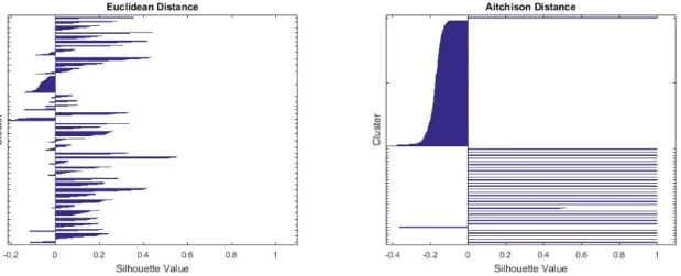
Figure 2.3 Silhouette value for each point with Euclidean and Aitchison distances when

clustering 400 Image Dataset . . . 21

Figure 2.4 Silhouette value for each point with Euclidean and Aitchison distances when

clustering text data. (N)is 50 . . . 21

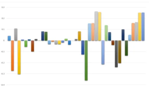
Figure 2.5 Score obtained after applying weight by maximum relevance feature

selec-tion technique. . . 22

Figure 2.6 Score obtained after applying LASSO feature selection technique. . . 22

Figure 2.7 Accuracy of DMM model using different approaches. . . 23

Figure 3.1 Segmentation of images from Berkeley 500 database. Column 1 gives the

original image, column 2: Noisy Image, Column 3: Segmentation with Gaussian

Mixture model, Column 4: Segmentation with Dirichlet Mixture model, Column 5:

Segmentation with Markov Random field with Gaussian mixture model and Column

6: Proposed method with Dirichlet mixture model. . . 38

original image, column 2: Noisy Image, Column 3: Segmentation with Gaussian

Mixture model, Column 4: Segmentation with generalized Dirichlet Mixture model,

Column 5: Segmentation with Markov Random Field with Gaussian mixture model

and Column 6: Proposed method with generalized Dirichlet mixture model. . . 39

(9)

original image, Column 2: Segmentation with Markov Random Field with

Gaus-sian mixture model, Column 3: Proposed method with Dirichlet mixture model and

(10)

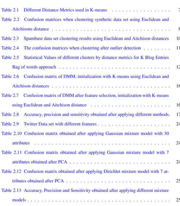
List of Tables

Table 2.1 Different Distance Metrics used in K-means . . . 7

Table 2.2 Confusion matrices when clustering synthetic data set using Euclidean and

Aitchisons distance . . . 8

Table 2.3 Spambase data set clustering results using Euclidean and Aitchison distances 10

Table 2.4 The confusion matrices when clustering after outlier detection . . . 11

Table 2.5 Statistical Values of different clusters by distance metrics for K Blog Entries

Bag of words approach . . . 12

Table 2.6 Confusion matrix of DMM, initialization with K-means using Euclidean and

Aitchison distances . . . 16

Table 2.7 Confusion matrix of DMM after feature selection, initialization with K-means

using Euclidean and Aitchison distance . . . 16

Table 2.8 Accuracy, precision and sensitivity obtained after applying different methods. 17

Table 2.9 Twitter Data set with different features. . . 24

Table 2.10 Confusion matrix obtained after applying Gaussian mixture model with 30

attributes . . . 24

Table 2.11 Confusion matrix obtained after applying Gaussian mixture model with 7

attributes obtained after PCA . . . 24

Table 2.12 Confusion matrix obtained after applying Dirichlet mixture model with 7

at-tributes obtained after PCA . . . 25

Table 2.13 Accuracy, Precision and Sensitivity obtained after applying different mixture

models . . . 25

(11)

Table 3.1 NPR index sample for Gaussian Mixture model (GMM), Dirichlet Mixture

model (DMM), Fast and Robust Gaussian mixture model (FRGMM) and Fast and

Robust Dirichlet mixture model (FRDMM) . . . 37

Table 3.2 NPR index sample for Gaussian Mixture model (GMM), generalized Dirichlet

Mixture model (GDMM), Fast and Robust Gaussian mixture model (FRGMM) and

Fast and Robust generalized Dirichlet mixture model (FRGDMM) . . . 41

Table 3.3 NPR index sample for Fast and Robust Gaussian mixture model (FRGMM),

Fast and Robust Dirichlet mixture model (FRDMM) and Fast and Robust

(12)

Chapter 1

Introduction

1.1 Introduction and Related Work

Data clustering is one of the main problems in data mining. It is an unsupervised classification of patterns (observations, data items or feature vectors) into groups (clusters) (34). Data clustering

is used in computer vision, decision making, pattern analysis and machine learning applications such as image segmentation, information retrieval, anomaly detection and character recognition. Due to the advancement of technology, a huge amount of data is generated every day. Proportional data, in particular, are naturally generated by different fields such as geology, Bio-informatics, com-puter vision, etc. Proportional data can be defined as any vectorx= (x1, x2..., xD)subject to unit

sum constraint where(x1+x2...+xD) = 1andxd ≥ 0,d = 1,2, ..., D. The clustering of this

type of data requires efficient algorithms (39). Cluster analysis is prevalent in any discipline that

involves analysis of multivariate data (34). The problem of unsupervised clustering using mixture

models requires good initialization which is generally done with the help of K-means algorithm. However, K-means uses Euclidean distance which finds the shortest distance between two sam-ples. Unfortunately, the Euclidean distance is not appropriate for proportional data. Despite the fact that Aitchison and other distance metrics are appropriate for proportional data, they have not re-ceived much attention compared to Euclidean distance. However, some related works do exist. For instance, Kashima et al. proposed a L1 distance (36) based K-means algorithm to address the

prob-lem of proportional vectors clustering. Hijazi et al. used Dirichlet regression models for modeling

(13)

compositional data and came to the conclusion that Dirichlet regression model is just an alternative to log-ratio analysis which can be done by Aitchison Log Ratio Analysis (30). In this thesis, I have

compared different distance metrics when clustering proportional data with K-means algorithm. A direct application of clustering is intrusion detection. Emerging growth of networks and rate of transfer of data through networks has increased the demand for network security. Machine learn-ing approaches are one of the popular strategies in network security for findlearn-ing attacks. The NSL-KDD data-set is widely used to validate network intrusion detectors, a predictive model capable of distinguishing between ’bad’ connections, called intrusions or attacks and ’good’ normal con-nections. There is a significant literature on Anomaly detection. Anomaly detection deviates from normal traffic and it is important to find an anomaly in an era of communication. Although, there are a lot of articles on intrusion detection, feature selection and unsupervised learning approaches are often underrepresented. There are very limited publicly available data sets for network-based anomaly detection. Earlier KDDCup99 was used heavily for all kind of intrusion detections through machine learning methodology. KDDCup99 has a huge number of redundant records (54). It was

found that around 78% of records in KDDCup99 were duplicated. Mchugh (43) gave many

crit-ics on KDDCup dataset and DARPA data set of 1998 as it was not good for applying statistical approaches to learning. The new NSL KDD data set was proposed (5) to overcome the problems

present in KDDCup99 and DARPA data sets (1). NSL KDD data set does not have redundant and

duplicate records. There is a lot of work which has been done on NSL KDD data set to find in-trusions. All existing learning approaches are supervised. The author in (29) had used principle

component analysis for feature extraction followed by SVM for finding intrusions in NSL KDD data set. The author in (46) had used a combination of classifiers or clusters which are followed by

supervised or unsupervised data filtering. The author in (64) had used feature selection with NSL

KDD data set. In this thesis, we have used unsupervised learning using Dirichlet Mixture Model. The initialization of mixture model is done with K-means using different distance metrics. Aitchi-son distance metric showed better results than Euclidean distance. It is followed by feature selection on NSL KDD data which reduces features from 41 to 16 features. The comparative analysis has been drawn which shows how feature selection and proper initialization increases the detection rate in NSL-KDD data set.

(14)

Another direct application of clustering is image segmentation. It plays an important role in the field of computer vision, pattern recognition, and image processing. There has been a rapid growth in the domain of image segmentation. There are numerous methodologies being proposed and most of them are based on supervised approaches, with the availability of ground truth of image data sets like Berkeley data set, MIT image data sets, etc. In unsupervised approaches, the Gaussian distribution is heavily used for image segmentation purposes. However, it suffers from various limi-tations as discussed in (17). There are other models which have been proposed such as Dirichlet and

generalized Dirichlet mixtures that provide better results for compactly supported data as discussed in (26) (42). The generalized Dirichlet mixture model has more flexible covariance structure and

requirements of conditional independence are less restrictive as compared to the Dirichlet mixture model (61).

Previously, The Dirichlet and generalized Dirichlet mixture models have been deployed for image processing, clustering and various other pattern recognition applications (14) (13) (60). The

Markov random field for image segmentation has been used in the past to find color boundaries (31). It has been used to eliminate noise and to fill in data without disrupting its discontinuities (8).

Markov random field (MRF) uses image brightness of edges as its guide to find contours. Hence, this property of MRF has integrated with Gaussian mixture models using Expectation-Maximization technique in (44). In the segmentation approach proposed in this thesis, the integration of spatial

information using MRF in Dirichlet and generalized Dirichlet mixtures is applied. To the best of our knowledge, this technique has not been used before for these mixtures. This combination aims to enhance image segmentation. The comparative results obtained are very encouraging.

1.2 Contributions

The contributions of the thesis are as follows:

(1) Comparing different distance metrics for K-means clustering of proportional data: In the proposed work, we present the K-means clustering approach using different distance met-rics. In particular, we propose the consideration of the Aitchison’s distance. Experimental

(15)

results are presented using silhouette plots for showing divergence from the center, and confu-sion matrices are used to validate our clustering of synthetic and real data sets. The algorithm with Aitchison’s distance metric results in lower error rates.

(2) Proposing k-means with feature selection to improve mixture model accuracy, sensitiv-ity and precision: Most of the approaches applied on a NSL KDD data set were supervised approaches. We had conducted statistical analysis on this data set using a Dirichlet Mixture model. We have performed initialization using Aitchison’s distance metric. The feature se-lection highly affects both the performance and results leading to an improved evaluation of anomaly detection through an unsupervised approach.

(3) Integration of spatial Information into Dirichlet and generalized Dirichlet finite mixture models: Our approach suggests the integration of spatial information into two different finite mixture models (Dirichlet mixture model, generalized Dirichlet mixture model) to produce smooth and more meaningful regions in image segmentation while offering more flexibility and ease of use for data modeling in comparison to the well known Gaussian mixture model.

1.3 Thesis Overview

(1) Chapter 1: It introduces the thesis and gives some related works. This presents the predica-ment of clustering data sets in unsupervised learning.

(2) Chapter 2: It proposes new distance metrics that can be used in a K-means clustering algo-rithm which is capable of clustering proportional data sets. It proposes how proper initializa-tion in mixture models using the above proposed method improves the results via an intrusion detection application. Hence, further improvement is depicted using feature selection and feature extraction methods.

(3) Chapter 3:This chapter shows the integration of spatial information using Markov Random Field into mixture models. The results have shown increased improvements when compared with similar previous approaches.

(16)

Chapter 2

Proportional Data Clustering using

K-Means Algorithm: A comparison of

different distances

In this work, we propose to use Aitchison distance metric for clustering of proportional data (6). Moreover, we compare it with several other distances in several applications. The rest of the

chapter is organized as follows: In section 2.1, the proposed method is explained in details, and

various distance metrics are introduced. In section2.2, outlier detection method with the proposed

algorithm is proposed. Section2.3gives different experimental results on many synthetic and real

data sets. Finally, in section2.6concluding remarks are drawn.

2.1 The Proposed Method

K-means clustering uses distance metrics to find nearest neighbors and mostly Euclidean dis-tance has been used. The objective function of K-means can be represented as follows:

J = k X j=1 n X i=1 x j i −cj 2 (1)

In this equation xi represents the data point andcj represents the cluster center. This type of

(17)

distance generates spherical shaped type of clusters as a result. Kashima et al. (36) proposedL1 distance which is also known as Manhattan distance for optimization of K-means clustering on proportional data and successful improvement was seen. There are many different distances and divergence metrics. However, in our chapter we concentrated on Euclidean log transformed data, Aitchison’s and Kullback-Leibler divergence. These distances have been known for a long time, but they have not been explored for proportional data. The only drawback of these distances is that they don’t accept 0 values. Martin et al. (40) proposed an approach to deal with zeros in compositional

data. We have applied this approach before clustering. In this chapter, we are proposing K-means clustering using Aitchison distance. As per our knowledge, this distance has not been considered in K-means in the past.

Algorithm 1K-means Algorithm

1: Set the Initial number of centroids randomly or sequentially.

2: Calculate the distance between each data point and cluster centers.

3: repeat:

4: Assign the minimumdistance data pointsto cluster center whose distance is minimum to that point.

5: Recalculate the cluster center using:

6: ci = _m1_iPjm=1i x(i);mi represents total number of data points in(i)cluster.

7: Re-calculate the distance between each data point and newly obtained cluster center.

8: until: No data point is reassigned.

In the K-means algorithm, distance is used in steps 2 and 4 of Algorithm1. The distance metrics

that we have explored are given in Table2.1.

2.2 Outlier Detection

Outlier detection is a deeply researched topic in both communities of statistics and data mining (21). Outlier detection methods are categorized as external and internal methods (63). In our case,

we used internal outlier detection technique where after K-means clustering with various distance metrics, distance is compared with the other data in same group with centroids of particular group as shown in Algorithm2.

(18)

Table 2.1: Different Distance Metrics used in K-means S.No. Distance Name Distance Metrics

1 Euclidean Distance d2_E(x, y) =P i(xi−yi) 2 2 EL transformed Data d2 EL(x, y) = P i(logxi−logyi)2 3 J-divergence d2_jd(x, y) =P i(logxi−logyi) (xi−yi) 4 Jeffery’s-Matusita Distance d2_m(x, y) =P i √ xi− √ yi 2

5 Manhattan Distance (L1 Distance) d2_L₁(x, y) =P

i|xi−yi|

6 Kullback-Leibler Divergence dKL(x, y) =Pi

xilogx_y_ii +yilogy_xi_i

7 Aitchison’s Distance dAD(x, y) = _D1 P_i<j

logxi xj −log yi yj d2_AD(x, y) =PD k=1 log xi g(xj)−log yi g(yj) 8 Cosine Distance dC(x, y) = 1− P ixiyi √ P ix2i √ P iy2i 9 Mahalonbis Distance d2_m(x, y) = (x−y)TS−1(x−y)

Algorithm 2Outlier Detection Algorithm

1: Perform K-means Algorithm (Algo. 1 )

2: INPUT: D-Dimensional DataXn, n = 1, ..., N, No of Clusters and choose distance metrics

(Aitchison Distance) for K-means.

3: Find distance between obtained centers and points using distance metrics.

4: Sort in descending order the distance obtained.

5: dmax =maxi{kxi−cik}, i= 1...N

6: Highest distance between center and points is an outlier.

2.3 Experiments with Synthetic and Real Data

2.3.1 Synthetic Data sets:

We have taken synthetic data set to validate our proposed method. We have generated samples of data using 2 different mixtures of Dirichlet distributions by using differentα parameters. This synthetic data set consists of 400 vectors with a dimension of 100. The Dirichlet distribution can be expressed as:

(19)

p(X|α) = 1 β(α) K Y i=1 xαi−1 i (2) β(α) = Qk i=1Γ (αi) ΓPk i=1αi (3)

Over here in above equation α = (α1, ..., αK). When we performed K-means clustering with

Euclidean and Aitchison distance matrices the results obtained are shown by confusion matrices in Table2.2. it is clear that Aitchison distance is much better for proportional data clustering.

Table 2.2: Confusion matrices when clustering synthetic data set using Euclidean and Aitchisons distance

K-means Euclidean distance) Yes No Yes 155 45 No 200 0

K-means Aitchison distance Yes No Yes 90 110 No 105 95

2.3.2 Real Data sets:

In our experiments we have taken three real data sets for clustering. The data sets are:

• Data set 1 (Text Documents) (3) Instances: 3430

Vocabulary words: 6906

Number of words in collection: 467714. Number of Classes: 50

• Data set 2 (Spambase) (4) Instances: 4601

Attributes: 57

(20)

• Data set 3 : Human Face Identification (49) Number of Facial expression: 400 images Dictionary size: 1000

classification is 40.

The first experiment is on document clustering using bag of words approach. We have taken the KOS blog entries (3) as our data set which contains 3430 documents and number of words in the

vocabulary is 6906. The problem arises with value of zeros in the data-sets. So, before performing clustering we removed 0 values by using exponentially small value around2(−52). After processing, we normalize data using following equation:

xi =

xi x1+x2....+xD

(4)

The second experiment is on visual objects clustering using bag of visual words approach. The real image data set contains 400 images of 256 pixels each presenting facial expressions. In order to generate bag of visual words, SIFT descriptor (51) has been used. After this process, each image

is represented as a proportional vector.

Figure 2.1: Data set 3 contains 400 facial images of 40 individuals, each showing 3 different but similar facial expressions. (49)

(21)

dimensional clustering is with the help of Silhouette. Peter J.Rousseew (48) explains how the cluster

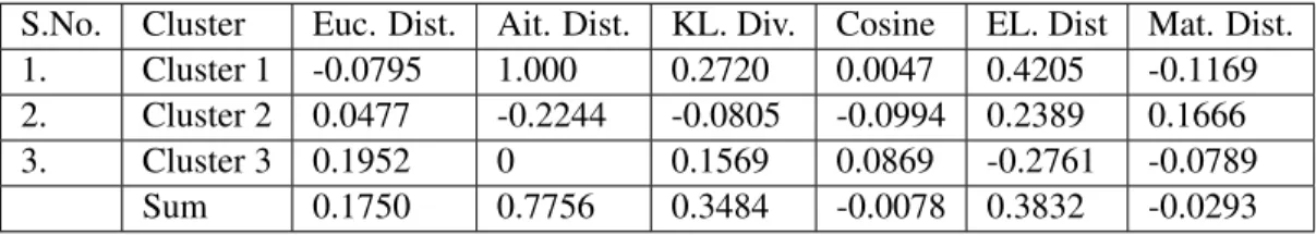
analysis can be done with the help of silhouette. Silhouette is a method which is used to find the consistency of clustered data. The values obtained for each vector can be combined and statistical values can be obtained to validate the clustering operation. The statistical values ranges between -1 to 1, and show how an object is well matched to its own cluster. Higher silhouette value means the clustering is appropriate. If a negative value is obtained it means more clustering can be done and the points does not lie within the same clusters. After finding the silhouette value it is necessary to find the group wise summary statistics which gives us a clear view of clustering. Table2.5 shows

the statistical values for clustering using different distance metrics of KOS blog entries. Our results for text clustering shows that the Aitchison distance metrics is most appropriate among all, as the higher silhouette value the more appropriate is the clustering. It is followed by Kullback distance metric and then Euclidean log distance metric. The Euclidean, Matisuita and the cosine show the poorest results for proportional data clustering, while, Cosine distance gives good results when data set is in form of frequency. For Spambase (4), we have obtained good results.

Table 2.3: Spambase data set clustering results using Euclidean and Aitchison distances K-means Euclidean distance)

Yes No Yes 345 1468 No 952 1836

2.3.3 Outlier detection results:

We have used Haberman’s survival dataset for finding outliers. The data set consists of 306 instances and 3 attributes. Through the results obtained k-means with Aitchison distance was able to determine 5 outliers correctly whereas k-means with Euclidean distance determined 3 outliers correctly. Table 2.4 shows the confusion matrix after performing the experiment and figure 2.2

(22)

Table 2.4: The confusion matrices when clustering after outlier detection K-means Euclidean distance)

Yes No Yes 121 47 No 102 31

2.3.4 Error percentage:

To find error percentage Silhouette method is used as given by equation 5. In this equation,

a(i) is the average dissimilarity within the same cluster, b(i) is lowest average dissimilarity ofi

to any other cluster where as iis a datum. It is used to find total sum of the silhouette values of each cluster on a data set. The error percentage is used to the dissimilarity of the clustered data as given by equation6. It represents group wise statistics where mean of each cluster silhouette value

is calculated andx¯gives the sum of the mean of silhouette value of each cluster. In equation7, we find error percentage or dissimilarity percentage of K-means clustering based on distance metrics.

s(i, j) =           

1−a(i) :a(i)< b(i) 0 :a(i) =b(i) b(i)/a(i) :a(i)> b(i)

(5) ¯ x= 1 N N X j=1 s(i, j) (6) e= N −x¯ N ×100 (7)

The above process was performed on facial image data set (49) of 400 images which has 40

different classes of 10 images each. The error percentage or dissimilarity measure obtained by clustering into 40 different clusters was 24.75 % by k-means using Aitchison distance and 32.66 % by K-means using Euclidean distance. Table2.5 provides the statistical values which are mean

of each silhouette value that clearly determines Aitchison distance is much better distance metric when compared to other distance metrics.

(23)

S.No. Cluster Euc. Dist. Ait. Dist. KL. Div. Cosine EL. Dist Mat. Dist. 1. Cluster 1 -0.0795 1.000 0.2720 0.0047 0.4205 -0.1169 2. Cluster 2 0.0477 -0.2244 -0.0805 -0.0994 0.2389 0.1666 3. Cluster 3 0.1952 0 0.1569 0.0869 -0.2761 -0.0789

Sum 0.1750 0.7756 0.3484 -0.0078 0.3832 -0.0293

Table 2.5: Statistical Values of different clusters by distance metrics for K Blog Entries Bag of words approach

2.4 Intrusion Detection System using Unsupervised Approach

In Section 2.4.1of our chapter, we discuss same feature selection approaches and results

ob-tained when applied to intrusion detection. In section2.4.2, Dirichlet mixture model is discussed

with Aitchison distance being applied on K-means. Section2.4.3, gives the experimental results.

2.4.1 Feature Selection:

There are various feature selection methods example include: Stepwise Regression, Stability Selection, Significance Analysis for Micro arrays, Weight by Maximum relevance, Least Abso-lute Selection and Shrinkage Operator (LASSO), etc. While feature selection performs removal of relevant features, feature extraction transforms the attributes where transformed attributes are com-bination of the original ones. In this process linear dependency between the features is minimized and projection of original data is on new space. The common feature extraction methods are PCA (principal component analysis), ICA (independent component analysis), Multi factor dimensional-ity reduction, Latent semantic analysis, etc. A novel method for feature extraction in the case of proportional data was proposed in (41) using data separation by Dirichlet distribution. In our work,

we have concentrated upon feature selection.

Weight by Maximum Relevance:

Weight by Maximum Relevance approach has been proposed in (10). It is a filter that measures

the dependence between every feature x and the classification feature y (i.e., the label) using Pear-son’s linear correlation, F-test scores and mutual information (33) (10). The high score by mutual

(24)

in order to reduce the complexity and finding an optimal solution we have reduced it to 16 features taking into an account that Weight by Maximum Relevance score of feature isf ≥0.05. The output obtained is displayed in figure2.5.

Weight by Maximum Relevance correlation vector can be defined by Pearson Correlation coef-ficient as:

R(i) = _p cov(Xi, Y) V ar(Xi)V ar(Y)

(8) The equation can be written as:

R(i) = PM k=1(xk,i−x) (y¯ k−y)¯ q PM k=1(xk,i−x)¯ 2PMk=1(yk−y)¯ 2 (9)

This can only detect the linear dependency between variable and target (28).

Least Absolute Selection and Shrinkage Operator (LASSO)

Least Absolute Selection and Shrinkage Operator (LASSO) has been proposed in (55). It is a

method which is used for estimation in Linear models. The method minimizes the residual sum of squares which is related to coefficient being less than a constant. It usesβ as a checking vector which is a coefficient vector. It shrinks coefficients and set others to zero, therefore tries to retain the good features of both subset selection and ridge regression. It is given (x1, x2, ..., xD) and

an outcome be y, the LASSO should fit linear model. The computation of LASSO is a quadratic problem and can be solved by standard numerical analysis algorithms. LASSO does shrinkage and variable selection where as in ridge regression only shrinkage takes place. The initial idea is to start working with large value ofλand slowly start decreasing it. The minimization for LASSO can be expressed as follow: f = n X i=1 (yi− X j xijβj)2+λ p X j=1 |βj| (10)

In this equationyi is the outcome variable, for casesi= 1,2, ..., nfeaturesxij,j = 1,2, ..., p.

Figure2.6. represents feature selection by LASSO and reducing features to 16 features by taking

(25)

2.4.2 Proposed Method LetX = n ~ X1, ~X2, ..., ~XN o

be a data set withN D-dimensional vectors modeled by a Dirichlet mixture model, then:

p ~ Xi|θ = M X j=1 pjp ~ Xi|~αj (11)

whereα~jis the parameter vector of component j,{pj}are the mixing proportions which should

be positive and always sum to 1.θ={p1, p2, ..., pM;~α1, ~α2, ..., ~αM}is the complete set of

param-eters fully characterizing the mixture, and M ≥ 1 is the number of components. Each Dirichlet distribution can be written in the form

pX~i|~αj = 1 β(α) D Y d=1 Xαjd−1 id (12) β(α) = QD d=1Γ (αjd) ΓPD d=1αjd (13)

whereXid > 0d = 1,2, ..., D,Xi1+Xi2, ...,+Xid = 1, and~αj = (αj1, αj2, ..., αjD)

rep-resents parameter vector forjth population. Let X be a data set with a common, but unknown, probability density functionp(X~i|θ)as given in above equation. We supposed that the number of

mixture components is known. The ML estimation method consists of getting the mixture param-eters that maximize log likelihood function. The below equation defines the posterior probability obtained after maximizing log likelihood function. This function is used in the E-step of Expectation Maximization (EM) algorithm.

p j|X~i, ~αj = pjp ~ Xi|α~j PK k=1pkp ~ Xi|~αk (14)

Now, using this expectation our goal is to maximize complete log likelihood. During the process we also have to ensure the constraintspj ≥0as well asPM_j₌₁pj = 1. In maximization step of the

algorithm, we have to update the parametersαuntil convergence to get the best result. As, it is to be noted that closed form solution forαdoes not exist. In the maximization step, iterative approach

(26)

of newton raphson method has been used as explained in (16).

During the initialization we use K-means algorithm as given in Algorithm 1. We have used

Euclidean and Aitchison distances. As, we know that Aitchison distance out performs Euclidean distance metric when proportional data are in question. In order to increase the performance of the algorithm, we have used feature selection methodology. In order to perform feature selection, the first step we have taken is to normalize the NSL KDD data set.

xi =

xi x1+x2....+xD

(15)

After obtaining proportional data, which act as an input for Weight by Maximum Relevance

(WMR) proposed by Blum et al. (10) and Least Absolute Selection and Shrinkage Operator

(LASSO)for selection of features from a data set.

Algorithm 3EM Algorithm for Dirichlet Mixture Model

1: Input:Data set

~

X1, ~X2, ..., ~XN

and specified number of components M.

2: Apply the k-means algorithm as given in Algorithm 1 on ND-dimensional vectors to obtain initial M clusters.

3: calculatepj =

Number of elements in class j N

4: Apply moments method to obtainαparameters.

5: Expectation-Maximization stepafter Initialization

6: E-Step: Compute the posterior probabilitypj|X~i, ~αj

7: M-Step:

8: repeat:

9: Update priorspj using equation14.

10: Update the parametersαusing Newton Raphson method.(16).

11: until:pj ≤, discardjand go to E-Step.

12: if convergence test is passed then terminate, else go to E-Step.

2.4.3 Experiment with NSL KDD data set

We have taken NSL KDD 2009 data-set for performing Intrusion detection. The NSL KDD data set contains 2 classes which are normal and attack sets. The attacks can be divided into four parts which are: Denial of Service Attack (DoS), User to Root attacks (U2R), Remote to local attacks (R2L) and probing attacks. In our experiment we have taken only normal and attack sets into consideration without considering different types of attacks. In our methodology, we have

(27)

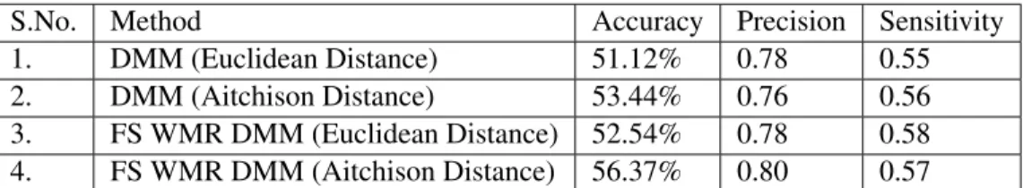
used Dirichlet mixture model for clustering. While performing clustering using Dirichlet mixture model results into 51.12% of accuracy which was relatively increased to 53.44 % when clustering was performed with initialization of k-means using Aitchison distance. In our experiments, we have done feature selection using the methodology of Weight by maximum relevance where the number of features has been reduced to 16 instead of 41. The experiment on 16 features using Dirichlet mixture model with Euclidean distance in K-means during initialization results into 52.54 % accuracy and 56.37 % was obtained when initialization was done with K-means using Aitchison distance as shown by figure 2.7 and by table2.8. To depict our results, we have used confusion

matrix (see Table2.6,2.7). Accuracy is defined as percentage of correctly classified vectors:

Accuracy= 100×Correctly identified vector

total vectors (16)

In our case we have used only test data without labels. Our results are better than SVM approach where accuracy determined is 51.90 % (33). The author in (25) obtained 47% which is comparably

less than our approach.

Table 2.6: Confusion matrix of DMM, initialization with K-means using Euclidean and Aitchison distances DMM (Euclidean distance) Yes No Yes 5386 1492 No 4300 672 DMM (Aitchison distance) Yes No Yes 4953 1564 No 3953 1380

Table 2.7: Confusion matrix of DMM after feature selection, initialization with K-means using Euclidean and Aitchison distance

Confusion Matrix FS WMR DMM (Euclidean distance)

Yes No Yes 5587 1513 No 4111 639

Confusion Matrix DMM (Aitchison distance) Yes No

Yes 5128 1285 No 3884 1553

(28)

S.No. Method Accuracy Precision Sensitivity 1. DMM (Euclidean Distance) 51.12% 0.78 0.55 2. DMM (Aitchison Distance) 53.44% 0.76 0.56 3. FS WMR DMM (Euclidean Distance) 52.54% 0.78 0.58 4. FS WMR DMM (Aitchison Distance) 56.37% 0.80 0.57

Table 2.8: Accuracy, precision and sensitivity obtained after applying different methods.

2.5 Bot detection using Mixture model for twitter tweets

In today’s era, social media has taken its leap in every phase of life and become a part of everyday activities being elections, marketing, etc. It is an important tool for public policy as seen from examples such as Arab spring, japan earthquake, etc. Micro blogging websites like twitter, tumblr, etc are used to display smaller content which are useful in SEO (Search Engine Optimization) point of view. Twitter has become relatively popular as it gives real time information. Even major search engines like Google, Bing, etc uses twitter data for mining real time events happening around the world. As only 140 characters are allowed on twitter which are used by major companies to analyze these short messages being it media, marketing companies, etc. The trending topic on twitter is taken as an advantage by spammers or bot’s to post pictures, tweets containing shortened URL which takes the user to unrelated websites. Hence, until now no proper mechanism has been found. In web services, phishing and malware attacks are the regular threats. The new methodologies in this domain by using unsupervised learning approach should be devised to counter such attacks. As, supervised learning consume lot of time and training cost. In the last decade there has been rapid shift from the static, editor-controlled Web 1.0 to the user-driven Web 2.0 paradigm (53). The web 2.0 allows us to post any type of content which becomes the target for

spammers. The spam or bot has also been developed on mobile applications.

There is lot of research being done on twitter primarily on twitter sentiment analysis (37), (58)

which is related to linguistics depicting emotions. There has been very little research conducted for detecting social spammers on twitter such as creation of duplicate accounts, automatic tweets at set amount of time which affects public opinion in making decision. The authors in (38) used machine

learning approach to create classifier for identification of spam. Another research done by author in (57) used Bayesian classifier to detect spam and non spam tweets. The famous research done by

(29)

author in (7) has collected billions of tweets from many different users and used SVM to classify

spam or fake tweets.

All research done has focused on the use of supervised learning approaches. Supervised learning is usually not that much practical for online, ever changing, inconsistent data. Thus, we propose the use of unsupervised technique on such type of data to detect bots on twitter tweets of Colombian election. The results obtained are motivating and better than most of the supervised approaches proposed previously.

In this section, we use unsupervised approach using Dirichlet mixture model. Feature extraction method is used to reduce the features from the data set and they are reduced from 30 to 7.

2.5.1 Experimental Results

In our experiment we have compared our approach with Gaussian mixture model. We have taken Colombian election twitter tweets (19) and our main goal is to cluster the data in order to

decide whether the tweet has been generated by the bot or it has been manually tweeted by the person. The bot tries to masquerade like humans and its quite difficult to identify them with present models. The tweets are converted from text to numeric form by following the bag of words (BoW) approach.

After we use feature extraction method to obtain the set of values which are linearly uncorrelated variables into an orthogonal plane. The method we use as feature extraction is Principal Component Analysis (35). The main goal to utilize feature extraction is to increase the efficiency of mixture

model. Hence, feature extraction methodology is different from feature selection. In this case we don’t lose any information and it is just projection of data into a plane. By using Principal Component Analysis we obtain negative scores which can be converted to positive without affecting the magnitude of the values by findingval=max(x)−min(x)and dot product of thevalwith the datax. After which we use the normalizing equation to normalize the data again. The experiment shows that in unsupervised learning approach Dirichlet mixture model performs far better than Gaussian mixture model. The initial data we have consist of 1331 users with 30 attributes which consist of most recent tweets by the users. Over here we are taking 40 most recent tweets of each user and it can be depicted as follow:

(30)

The feature extraction step has reduced the features to 7. The various measures used to deter-mine our results are as follows:

Accuracy= TP+TN T P +F P +T N+F N (17) P recision= TP T P +F P (18) Sensitivity = TP T P +F N (19)

The results obtained shows that accuracy has considerably increased by applying Principal com-ponent analysis. The Dirichlet mixture model outperforms Gaussian mixture model in terms of de-tecting bot tweets on collected twitter data. The reported result obtained by Dirichlet mixture model is 66.79% where as precision and sensitivity have also increased.

2.6 Conclusion

Different distance metrics have been investigated for the K-means clustering of proportional data. Aitchison distance has been shown to give the best performance. This distance can be used with different types of clustering methodologies. The proper initialization for mixture models is a crucial step in unsupervised learning. Using Aitchison distance as initialization step can give better mixture results applicable to proportional data. It has also been observed that Aitchison distance performs better for sparse data sets and for high dimension when compared with Euclidean distance for this particular type of data. By finding the K-means score it has been seen that Aitchison’s distance is more viable solution as a distance metric for doing K-means clustering for proportional data. We have statistically analyzed the entire NSL KDD data set. In NSL KDD data set, 16 features had shown strong contribution for anomaly detection. Our basis is to state the baseline for unsupervised learning for future IDS solution

(31)

(32)

Figure 2.3: Silhouette value for each point with Euclidean and Aitchison distances when clustering 400 Image Dataset

Figure 2.4: Silhouette value for each point with Euclidean and Aitchison distances when clustering text data.(N)is 50

(33)

Figure 2.5: Score obtained after applying weight by maximum relevance feature selection technique.

(34)

(35)

S.No. Features

1. Profile description.

2. Verified: when 1, ”indicates that the user has a verified account.” 3. Age of the user account

4. Number of followings. 5. Number of followers

6. reputation= ₍_{number of followings + number of followers}(number of followers) ₎

7. User Mention

8. Unique user mention (@) ratio. 9. URL ratio.

10. Hashtag () ratio.

11. Average of tweet content similarity. 12. Retweet rate.

13. Reply rate. 14. Number of tweets.

15. Mean of inter-tweeting delay.

16. Standard deviation of inter-tweeting delay. 17. Average of tweets per day.

18. Average of tweets per week.

19. Number of tweets from manual devices. 20. Number of tweets from automated devices. 21. Fofo rate= _{number of followings}number of followers

22. Following rate= _{age of the user account (in days)}number of followings

23. Percentage of tweets posted during the 00:00:00 at 02:59:59 hours period. 24. Percentage of tweets posted during the 03:00:00 at 05:59:59 hours period. 25. Percentage of tweets posted during the 06:00:00 at 08:59:59 hours period. 26. Percentage of tweets posted during the 09:00:00 at 11:59:59 hours period. 27. Percentage of tweets posted during the 12:00:00 at 14:59:59 hours period. 28. Percentage of tweets posted during the 15:00:00 at 17:59:59 hours period. 29. Percentage of tweets posted during the 18:00:00 at 20:59:59 hours period. 30. Percentage of tweets posted during the 21:00:00 at 23:59:59 hours period.

Table 2.9: Twitter Data set with different features

A B

A 216 382 B 416 317

Table 2.10: Confusion matrix obtained after applying Gaussian mixture model with 30 attributes Yes No

Yes 337 221 No 303 430

Table 2.11: Confusion matrix obtained after applying Gaussian mixture model with 7 attributes obtained after PCA

(36)

Yes No Yes 598 135 No 307 291

Table 2.12: Confusion matrix obtained after applying Dirichlet mixture model with 7 attributes obtained after PCA

S.No. Process Accuracy Precision Sensitivity

1. GMM 40.00% 27.00% 34.17%

2. GMM (7 Attributes) 57.62% 60.39% 52.65% 3. DMM (7 Attributes) 66.79% 81.58% 66.07%

(37)

Chapter 3

Spatially Constrained Mixture Models

for Image Segmentation

The problem of image segmentation and grouping based on regions has remained as a great challenge in the field of computer vision. It is often the first step in variety of computer vision and image analysis tasks. There are various types of images we encounter in everyday life, for example, light intensity images, magnetic resonance image, etc (45). There has been a large number of

approaches proposed in previous years for image segmentation. The problem of image segmentation of noisy images or corrupt images is still an open challenge. Image segmentation is widely used for anomaly detection (18) and medical image analysis (47). Various statistical models have been

proposed in the past.

In this chapter, we develop an unsupervised approach for noisy image segmentation. Earlier similar unsupervised approaches have been used in research, for example, the author in (22) has

used fuzzy c-means for medical image segmentation. In this chapter, we had the focus on a par-ticular statistical model which is finite mixture. The main problems faced were 1) Integration of Markov Random Field (MRF) with Dirichlet based mixture models to achieve the segmentation of noisy images, 2) Estimation of parameters which is often a difficult task in mixture models, and 3) Initialization of parameters where we have used moments method with k-means. Markov Ran-dom Field has been heavily used for modeling spatial information for medical image segmentation

(38)

(27). Markov Random Field is heavily used for semantic segmentation of images in supervised

learning approaches which is defined as multi-label classification problem. An interesting approach to integrate spatial information with Gaussian distribution has been proposed in (62). As we know,

Gaussian mixture is a popular model in the field of computer vision. The Gaussian mixture model is restrictive as we have seen from previous works (52) (11) where Dirichlet and generalized Dirichlet

distributions have generally shown better results.

Hence, In this chapter, we propose the integration of Markov Random Field in Dirichlet and generalized Dirichlet mixture models which are flexible (52) for data modeling. Experiments show

that integrating spatial information into Dirichlet and generalized Dirichlet mixture models gives excellent results for image segmentation.

3.1 Dirichlet Mixture Segmentation approach

LetX =nX~1, ~X2, ..., ~XN

o

representing a given image whereN is the number of pixels and each pixel is denoted by random vector X~i = (Xi1, Xi2, ..., XiD). Now, the random vectorX~i

follows Dirichlet mixture model and is considered to be independent from the label. The density function can be presented as:

pX~i|θ = M X j=1 pjp ~ Xi|~αj (20)

whereα~jis the parameter vector of componentjwhich can be represented asα~j = (αj1, αj2, ..., αjD). {p_j}are the mixing proportions which should be positive and always sum to 1.

θ={p1, p2, ..., pM;α~1, ~α2, ..., ~αM}is the complete set of parameters fully characterizing the

mix-ture,M ≥1is the number of components.

p ~ Xi|~αj = 1 β(α) D Y d=1 X_idαjd−1 (21) β(α) = QD d=1Γ (αjd) Γ PD d=1αjd (22) where Xid > 0, d = 1,2, ..., D, Xi1 +Xi2, ...+XiD = 1, and ~αj = (αj1, αj2, ..., αjD)

(39)

distribution are given as follows: E(Xd) = αd |~α| (23) V ar(Xd) = αd(|~α| −αd) |~α|2+ 1 (24) Cov(Xi, Xj) = −α_iαj |~α|2(|~α|+ 1) (25)

The image is composed of different regions. Thus it’s appropriate to describe it by Dirichlet mixture model withM clusters as shown in equation20. Moreover, for each pixelX~i ∈ X, there

is a peer which has been arisen from the same cluster ofX~i. This spatial information can be used

indirectly to estimate the number of clusters or regions in an image.

3.1.1 Segmentation approach LetX =nX~1, ~X2, ..., ~XN

o

be a data set ofN D-dimensional positive vectors with a common, but unknown, probability density function p(X~i|θ) as given in 20. The vectors are modeled as

statistically independent, the joint conditional density of data can be presented as:

f(X |θ) = N Y i=1 p ~ Xi|θ = N Y i=1 M X j=1 pjp ~ Xi|~αj (26)

As we have taken each pixel to be independent of pixel label, the spatial correlation between nearby pixels is not taken into account. So, in this case, the image is relatively very sensitive to noise and illumination (50). To overcome the problem of noise and illumination the MRF (Markov

Random Field) is used to create the spatial correlation between label values. The MRF distribution is given by: f(Π) =Z−1exp −1 TU(Π) (27)

In MRF,Z is considered as normalizing constant,T is a Temperature constant andU(Π)is the smoothing prior whereΠ = pj. The Bayes rule for posterior probability can be represented as:

(40)

There has been vast research which has already been conducted for determining smoothing prior of MRF distribution. The smoothing prior determined in most research is complex and requires lot of computation time when combined with mixture models. The example of such kind of smoothing prior is given by (9): U(Π) =κ N X i=1 X m∈δi  1 +   M X j=1 (pij −pmj)2   −1  −1 (31)

whereκ represents a constant value. In the above equation,Z andT are set to 1 (Z = 1and

T = 1). Due to the complexity of this equation, the M-step of EM algorithm cannot be applied directly to prior distributionpj. Various smoothing priors were proposed, but the major drawback

of all of them has been that they are not robust to noise. In order to overcome this difficulty, prior distribution has been considered. A novel factor was proposed by (44) as follows:

Gt_ij = exp κ 2Ni X z_mj(t) +p(_mjt) (32)

In this equationκis the temperature value and hence, changing the temperature value determines noise reduction of the image. It is used to determine neighborhood pixels around the pixelXi. As

proposed by authors (44)Gij is only dependent on value of posteriors at previous step(t)and priors

value.

(41)

previously in smoothing prior. Hence, smoothing prior is given by: U(Π) =− N X i=1 M X j=1 G(_ijt)logp(_ijt+1) (33)

Maximizing equation30we get the expanded equation with the hidden variablezij

L(f(θ|X)) = N X i=1 M X j=1 z_ijt n logp(_jt+1)+ logp ~ Xi|~αj o −logZ +1 T N X i=1 M X j=1 Gt_ijlogp(_jt+1) (34)

The hidden variable can be expanded as

z(_ijt)= p(_jt)pX~i|~αj PK k=1p (t) k p ~ Xi|~αtk (35)

Hence, putting the value of U(Π) in equation30 and expanding the equation with Dirichlet distribution as well as setting normalizing constantZ and Temperature ValueT to be proportional over here (Z=1 andT=1), we get:

Q(f(θ|X)) = N X i=1 M X j=1 zt_ij ( logp(_jt+1)+ log Γ D X d=1 αt_jd+1 ! − D X d=1 log Γ (αjd)t+1+ D X d=1 αt_jd+1−1 log (Xid) + N X i=1 M X j=1 G(_ijt)logp(_jt+1) (36)

Now, In M-Step of Expectation Maximization algorithm,Qθ|X~is maximized using Newton-Raphson approach as proposed in (16). Hence, for the~αparameters we have:

α_jd(t+1) =α(_jdt)−H−1α(_jdt)×   ∂Qθ|X~ ∂αjd   (37)

(42)

mixed derivatives as presented in (16). To satisfy the condition ofPM

j=1pj = 1, we use the

La-grangian multiplierΛ, which gives:

pj = z_ij(t)+G(_ijt) Pk m=1 z_im(t)+G(_ikt) (38)

Now, we have done the integration of MRF into Dirichlet mixture model. Hence, we can see from the equation that MRF distribution is affecting the prior distribution which indirectly affects the estimation of the parameters.

3.1.2 Intialization and Segmentation Algorithm

Parameter initialization is important task for mixture models when parameter estimation is done through the EM algorithm. Our intialization algorithm is done through K-means using Aitchison distance metric and followed by method of moments (MM) algorithm (17). It can be summarized

as follows: αd= (x0₁₁−x0₂₁)x0₁_d x21−(x0₁₁)2 d= 1, ..., D (39) αD+1= (x0₁₁−x0₂₁) 1−PD d=1x 0 1d x0₂₁−(x0₁₁)2 (40) x0₁_d= 1 N N X n=1 xnd d= 1, ..., D+ 1 (41) x0₂₁= 1 N N X n=1 x2_n₁ (42)

Thus, the proposed learning approach is summarized in algorithm4:

3.2 Generalized Dirichlet Mixture Segmentation approach

It is known that Dirichlet distribution has its own limitations given by (14) (23) as it has negative

(43)

Algorithm 4EM Algorithm Dirichlet Mixture Model with MRF

1: Apply K-means on image data points to obtain initialkclusters for segmentation.

2: Initialization using Method of Moments as proposed by the author in (11) to obtainα parame-ters.

3: Use the image data points to update the mixture parameters.

4: E-Step: Compute the posterior probabilityz_ij(t)

5: M-Step:

6: repeat:

8: Update the parametersαusing Newton Raphson method (16).

of Dirichlet distribution. It can be given as follows:

p ~ X|~α = D X d=1 γ(αd+βd) γ(αd)γ(βd) Xαd−1 d 1− d X i=1 Xi !γd (43) for PD

d=1 Xd < 1and0 < Xd < 1 ford = 1,2, ..., D whereγd = βd−αd+1 −βd+1 for

d= 1, ..., D−1whereγd=βd−αd+1−βd+1ford= 1,2, ..., D−1andγd=βd−1. Note that

generalized Dirichlet distribution is reduced to a Dirichlet distribution whenβd = αd+1 +βd+1. The mean, variance and covariance can be shown as below:

E(Xd) = αd αd+βd d=1 Y i=1 βi+ 1 αi+βi (44) V ar(Xd) =E(Xd) αd+ 1 αd+βd+ 1 d=1 Y i=1 βi+ 1 αi+βi + 1−E(Xd) ! (45) Cov(Xi, Xj) =E(Xd) αi αi+βi+ 1 Y k=1 i= 1 βk+ 1 αk+βk + 1−E(Xi) ! (46)

The interesting applications for generalized Dirichlet distribution can be found in (59). The

approach can be explained as follows. For each pixelX~i∈ X, there is a peer which has been arisen

from the same cluster ofX~i. This spatial information can be used indirectly to estimate the number

(44)

3.2.1 Segmentation approach

In the following, we adopt the segmentation approach, based on generalized Dirichlet mixture models with Markov Random Field (MRF) for the introduction of spatial information. The density function can be presented as:

p ~ Xi|θ = M X j=1 pjp ~ Xi|~αj, ~βj (47)

where α~j, β~j is the parameter vector of component j which can be represented as ~αj = (αj1, αj2, ..., αjD) andβ~j = (βj1, βj2, ..., βjD). {pj} are the mixing proportions which should

be positive and always sum to 1. θ = np1, p2, ..., pM;~α1, ~α2, ..., ~αM, ~β1, ~β2, ..., ~βM

o

is the com-plete set of parameters fully characterizing the mixture,M ≥1is the number of components.

pX~i|~αj, ~βj = D Y d=1 Γ (αjd+βjd) Γ (αjd) Γ (βjd) Xαjd−1 id 1− d X K=1 XiK !γjd (48) where Xid > 0, d = 1,2, ..., D, Xi1 +Xi2, ...+XiD = 1, andα~j = (αj1, αj2, ..., αjD), ~

βj = (βj1, βj2, ..., βjD)represents parameter vector forjthcomponent. In this case, whereγjd = βjd−1, note that the generalized Dirichlet distribution is reduced to Dirichlet distribution (12) when βjd =αjd+1+βjd+1,d= 1, ..., D. LetX =

n

~

X1, ~X2, ..., ~XN

o

be a data set ofN D-dimensional positive vectors with a common, but unknown, probability density function p(X~i|θ) as given in

above equation. The vectors are modeled as statistically independent, the joint conditional density of data can be presented as:

f(X |θ) = N Y i=1 pX~i|θ = N Y i=1 M X j=1 pjp ~ Xi|~αj, ~βj (49)

As we have taken each pixel to be independent of pixel label, the spatial correlation between nearby pixels is not taken into an account. So, in this case, the image is relatively very sensitive to noise and illumination (50). To overcome the problem of noise and illumination the MRF (Markov

(45)

The log likelihood for generalized Dirichlet distribution is given as follow: L(f(θ|X)) = log (f(θ|X)) = N X i=1 log    M X j=1 pjp ~ Xi|~αj, ~βj    + logf(Π) (50) L(f(θ|X)) = N X i=1 log    M X j=1 pjp ~ Xi|~αj, ~βj    −logZ− 1 TU(Π) (51)

There has been vast research which has already been conducted for determining smoothing prior of MRF distribution. The smoothing prior determined in most research is complex and requires lot of computation time when combined with mixture models. The example of such kind of smoothing prior is given by (9) which is shown in equation31and33.

Maximizing equation51we get the expanded equation with the hidden variablezij

L(f(θ|X)) = N X i=1 M X j=1 z_ijt nlogp(_jt+1)+ logpX~i|~αj, ~βj o − logZ+ 1 T N X i=1 M X j=1 Gt_ijlogp(_jt+1) (52) where logpX~i|~αj, ~βj = D X d=1 [log Γ (αjd+βjd)]− D X d=1 [log (Γ (αjd) Γ (βjd))] + D X d=1 " αjd−1logXid−γjd d X K=1 logXiK # (53)

The hidden variable can be expanded as

z_ij(t)= p(_jt)pX~i|~αj, ~βj PK k=1p (t) k p ~ Xi|~α(_kt), ~β(_kt) (54)

Hence, putting the value of U(Π) in equation 51 and expanding the equation with general-ized Dirichlet distribution as well as setting normalizing constantZ and Temperature ValueT to

(46)

proportional over here (Z=1 andT=1) we get: Q(f(θ|X)) = N X i=1 M X j=1 zt_ijnlogp(_jt+1)o+ N X i=1 M X j=1 z_ijt {log (Γ (α_jd+βjd)−log (Γ (αjd) Γ (βjd)))} + N X i=1 M X j=1 z_ijt ( αjd−1logXid−γjd d X K=1 logXiK ) + N X i=1 M X j=1 zt_ijnG(_ijt)logpt_j+1o (55)

Now, In M-Step of Expectation Maximization algorithm,Qθ|X~is maximized using Newton-Raphson approach as proposed in (15). Hence, for the~α, ~βparameters we have:

   αjd βjd    (t+1) =    αjd βjd    (t) −H−1×    ∂Q(θ|_X~₎ ∂αjd ∂Q(θ|_X~₎ ∂βjd    (t) (56)

In the above equation H is the Hessian matrix which requires the calculation of second and mixed derivatives as presented in (15). To satisfy the condition ofPM

j=1pj = 1, we use the

La-grangian multiplierΛ. Using the above methods of prior probability which gives:

pj = z_ij(t)+G(_ijt) Pk m=1 z_im(t)+G(_ikt) (57)

Now, we have done the integration of MRF into generalized Dirichlet mixture model. Hence, we can see from the equation that MRF distribution is affecting the prior distribution which indirectly affects the estimation of the parameters.

3.2.2 Initialization and Segmentation Algorithm

Parameter initialization is an important issue in mixture models. The generalized Dirichlet mixture model initialization model has been proposed in (23). The integration of spatial information

(47)

Algorithm 5EM Algorithm for generalized Dirichlet Mixture Model with MRF

1: Apply K-means on image data points to obtain initialkclusters for segmentation as shown in Algorithm1.

2: Initialization using Method of Moments as proposed by the author in (15) to obtainα, β pa-rameters.

3: Use the image data points to update the mixture parameters.

4: E-Step: Compute the posterior probabilityz_ij(t)

5: M-Step:

6: repeat:

8: Update the parametersα,β using Newton Raphson method (15).

3.3 Experimental results

The main goal of this section is to investigate the performance of proposed method of Dirichlet and Generalized mixture models with Markov Random Field as compared with one developed by (44). The author in (44) has developed the model for Gaussian mixture with spatially constrained

information. The work has not been carried out for Non-Gaussian Mixture models which give relatively better results of image segmentation of noisy images. As, we have considered Dirichlet and Generalized model where Dirichlet mixture model is a special case of the generalized Dirichlet mixture model. Evaluating segmentation results is an important problem and over here we are using NPR (Normalized Probabilistic Rand) (56) which can be given as follows:

NPR Index= PR Index - Expected Index

Maximum Index - Expected Index (58)

The Expected value of PR Index can be given as follow:

E[P RI(Stest,{Sk})] = 1 N 2 X i,j i<j p0_ijpij 1−p0ij (1−pij) (59)

This comparison model was proposed in (56) in order to provide comparison between image

segmentation algorithms. In the experiment, the image is taken and converted to gray-scale after that we have induced three types of noise in an image which are: Gaussian noise, Poisson Noise

(48)

and Salt and Pepper. The Gaussian noise image de-noising was earlier proposed by (32) who used

soft threshold shrinkage method of sparse components. Poisson noise is also called as shot noise which is correlated with each pixel of an image. We add the Gaussian noise but Poisson is applied. Adaptive median filter with specialized regularization method has been used to reduce salt and pepper impulsive noises (20). We have observed that our method performs very well on all cases and

image segmentation takes place without any difficulty and even the proposed method of Dirichlet and generalized Dirichlet distribution is better than median based filters.

In our experiment conducted, we have set the temperature value(κ= 10). The other important factor in this equation is the determination of window size(Ni = 25). The data set used is Berkeley

Segmentation Data set 500 (BSDS500) which is an extension of Berkeley Segmentation data set 300 and BioId face database . These are publicly available data sets and heavily used in the field of computer vision. It is difficult to calculate NPR index of every image as this process is compu-tationally expensive so we have calculated NPR index of a limited number of images followed by different segmentation approaches. The experimental results show that there is a large difference between the two different mixture models used. Tables3.1,3.2and3.3show the NPR Index sample

mean of images by different mixture models being performed on images. It can be seen that inte-grated model with Dirichlet and generalized Dirichlet performs way better than modified Gaussian mixture model. Fig3.1shows the comparison of image segmentation results obtained after

apply-ing modified Dirichlet mixture model with the modified Gaussian mixture model. Fig3.2shows the

results of modified generalized Dirichlet mixture model with the modified Gaussian mixture model. Fig3.3shows the comparison of different images being segmented with different mixture models.

All of these approaches are applied on noisy images.

GMM DMM FRGMM FRDMM

NPR Index Sample Mean 0.2833 0.4024 0.5462 0.6022

Table 3.1: NPR index sample for Gaussian Mixture model (GMM), Dirichlet Mixture model (DMM), Fast and Robust Gaussian mixture model (FRGMM) and Fast and Robust Dirichlet mixture model (FRDMM)

(49)

Figure 3.1: Segmentation of images from Berkeley 500 database. Column 1 gives the original image, column 2: Noisy Image, Column 3: Segmentation with Gaussian Mixture model, Column 4: Segmentation with Dirichlet Mixture model, Column 5: Segmentation with Markov Random field with Gaussian mixture model and Column 6: Proposed method with Dirichlet mixture model.

(50)

Figure 3.2: Segmentation of images from Berkeley 500 database. Column 1 gives the original image, column 2: Noisy Image, Column 3: Segmentation with Gaussian Mixture model, Column 4: Segmentation with generalized Dirichlet Mixture model, Column 5: Segmentation with Markov Random Field with Gaussian mixture model and Column 6: Proposed method with generalized Dirichlet mixture model.

(51)

Figure 3.3: Segmentation of images from Berkeley 500 database. Column 1 gives the original im-age, Column 2: Segmentation with Markov Random Field with Gaussian mixture model, Column 3: Proposed method with Dirichlet mixture model and Column 4: Proposed method with generalized Dirichlet mixture model.

(52)

GMM GDMM FRGMM FRGDMM NPR Index Sample Mean 0.4530 0.4864 0.6012 0.6499

Table 3.2: NPR index sample for Gaussian Mixture model (GMM), generalized Dirichlet Mixture model (GDMM), Fast and Robust Gaussian mixture model (FRGMM) and Fast and Robust gener-alized Dirichlet mixture model (FRGDMM)

FRGMM FRDMM FRGDMM NPR Index Sample Mean 0.4522 0.5771 0.6074

Table 3.3: NPR index sample for Fast and Robust Gaussian mixture model (FRGMM), Fast and Ro-bust Dirichlet mixture model (FRDMM) and Fast and RoRo-bust generalized Dirichlet mixture model (FRGDMM)

3.4 Conclusion

In this chapter, we performed image segmentation based on Dirichlet and generalized Dirichlet mixture models with MRF (Markov Random field) to integrate the spatial information. It gave us good results when compared with modified Gaussian Mixture model. The generalized dirichlet mixture model is more flexible as it has two parameters when compared with Dirichlet mixture model. The selection of mixture model is motivated by its excellent results obtained when compared with other methodologies used in the past. The work can be extended for image segmentation with other mixture models and video segmentation being considered as another important application. Anomaly detection using video segmentation and learning approaches of the mixture can be done using for instance approaches previously proposed by (24). The drawback of a mixture model is

the initialization of parameters as proper initialization becomes complex due to complexity of the mixture.

(53)

Chapter 4

Conclusion

In this thesis, we have presented different distance metrics which can be used with a K-means algorithm for the clustering of proportional data and yet, they have not been exploited. We have shown how proportional data can be clustered using Aitchison’s distance which gives extremely good results. It was argued previously that Euclidean distance is not a universally defined distance to be used to measure distance between data points. We have shown how distance used with an initialization of Dirichlet distribution and generalized Dirichlet distribution gives better results. The above proposed method is exploited by using NSL-KDD data-set. This data-set is used for anomaly detection in network data. We have used feature selection methods such as LASSO and WMR after which mixture model is applied to get the results. The results had shown that Dirichlet mixture model works better when properly initialized.

In the second part of thesis, we have presented different algorithms for noisy image segmenta-tion by integrating spatial informasegmenta-tion using Markov random field (MRF) into finite mixture models. The selection of mixture models is motivated by their flexibility for approximation of data points in different shapes where a well known Gaussian mixture model always keeps the symmetric bell shape. Firstly, we have taken a Dirichlet mixture model for its flexibility and lower number of pa-rameters. We have initialized the parameters using a moments method by utilizing the Aitchison’s distance metric in K-means. The main drawback of Dirichlet mixture model is its negative covari-ance matrix. This disadvantage is handled by generalized Dirichlet distribution where number of parameters is increased. Both mixture models are applied for image segmentation by integrating

(54)

spatial information with MRF. To depict our results, we have used famous Berkeley Image data sets and our proposed algorithm performs better to deal with noise and illumination from an image. Future work can be devoted to an object detection and recognition. Video segmentation could be considered as another interesting application.

(55)

Abbreviations

GMM GaussianMixtureModel

DMM DirichletMixtureModel

GDMM GeneralizedDirichletMixtureModel

MRF MarkhovRandomField

PR ProbabilisticRand

NPR NormalizedProbabilisticRand

KL KullbackLeibler

EL EuclideanLogarithmic

LASSO LeastAbsoluteSelection andShrinkageOperator

WMR Weight byMaximumRelevance

Proportional Data Modeling using Unsupervised Learning and Applications