Learning local metrics and influential regions for classification

Dong, M., Wang, Y., Yang, X. and Xue, J.-H. (2020) Learning local metrics and

influential regions for classification. IEEE Transactions on Pattern Analysis and

Machine Intelligence, 42(6), pp. 1522-1529.

There may be differences between this version and the published version. You are

advised to consult the publisher’s version if you wish to cite from it.

http://eprints.gla.ac.uk/225908/

Deposited on: 5 November 2020

Enlighten – Research publications by members of the University of Glasgow

Learning Local Metrics and Influential Regions

for Classification

Mingzhi Dong, Yujiang Wang, Xiaochen Yang, Jing-Hao Xue

F

Abstract—The performance of distance-based classifiers heavily de-pends on the underlying distance metric, so it is valuable to learn a suitable metric from the data. To address the problem of multimodality, it is desirable to learn local metrics. In this short paper, we define a new intuitive distance with local metrics and influential regions, and subsequently propose a novel local metric learning algorithm called LM-LIR for distance-based classification. Our key intuition is to partition the metric space into influential regions and a background region, and then regulate the effectiveness of each local metric to be within the related influential regions. We learn multiple local metrics and influential regions to reduce the empirical hinge loss, and regularize the parameters on the basis of a resultant learning bound. Encouraging experimental results are obtained from various public and popular data sets.

Index Terms—Distance-based classification, distance metric, metric learning, local metric.

1 I

NTRODUCTION

C

LASSIFICATIONis a fundamental task in the field of machine learning. While deep learning classifiers have obtained supe-rior performance on numerous applications, they generally require a large amount of labeled data. For small data sets, traditional classification algorithms remain valuable.

The nearest neighbor (NN) classifier is one of the oldest estab-lished methods for classification, which compares the distances between a new instance and the training instances. However, with different metrics, the performance of NN would be quite different. Hence it is very beneficial if we can find a well-suited and adaptive distance metric for specific applications. To this end, metric learning is an appealing technique. It enables the algorithms to automatically learn a metric from the available data. Metric learning with a convex objective function was first proposed in the seminal work of Xing et al. [1]. After that, many other metric learning methods have been developed and widely adopted, such as the large margin nearest neighbor (LMNN) [2] and the informa-tion theoretic metric learning [3]. Some theoretical work has also been proposed for metric learning, especially on deriving different generalization bounds [4]–[7] and deep networks have been used to represent nonlinear metrics [8], [9]. In addition, metric learning methods have been developed for specific purposes, including multi-output tasks [10], multi-view learning [11], medical image

M. Dong, X. Yang and J.-H. Xue are with the Department of Statistical Science, University College London, London WC1E 6BT, UK (e-mail: [email protected]; [email protected]; [email protected]).

Y. Wang is with the Department of Computing, Imperial College London, London SW7 2AZ, UK (e-mail: [email protected]).

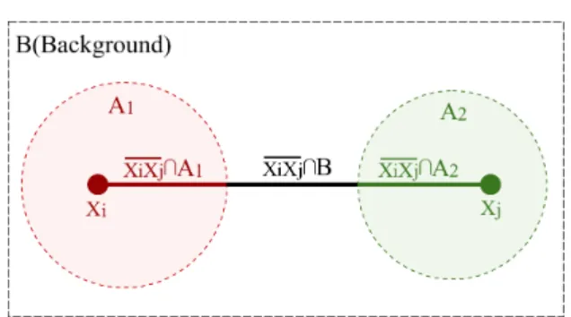
Fig. 1. An example of calculating the distance between two pointsxi andxj.A1andA2are different influential regions with metricsM(A1)

andM(A2), and B is the background region with metric M(B). The

distance betweenxiandxjequals to the sum of three line segments’ local distances, i.e.l(xixj\A1;M(A1)), l(xixj\A2;M(A2))and

l(xixj\B;M(B)).

retrieval [12], kinship verification tasks [13], face recognition tasks [14], tracking problems [15] and so on.

Most aforementioned methods use a single metric for the whole metric space and thus may not be well-suited for data sets with multimodality. To solve this problem, local metric learning algorithms have been proposed [2], [16]–[23].

Most of these localized algorithms can be categorized into two groups: 1) Each data point or cluster of data points has a local metric M(xi). This, however, results in an asymmetric distance as illustrated in [17], i.e.M(xi)6=M(xj)would cause

D(xi,xj;M(xi)) =6 D(xj,xi;M(xj)). 2) Each line segment or cluster of line segments has a local metric, i.e.M(xi,xj). In [19],M(xi,xj) = Pkwk(xi,xj)Mk, wherewk is defined as

P(k|xi)+P(k|xj)so as to guarantee the symmetry andP(k|xi) orP(k_|xj)is based on the posterior probability that the pointx belongs to thekth Gaussian cluster in a Gaussian mixture (GMM). However, most of the line segment approaches are based on certain heuristic design. Geometric properties of line segments, which are very intuitive and interpretable, have scarcely been considered.

In this short paper, we define a geometrically interpretable, symmetric distance, and propose a novel local metric learning algorithm that learns local metrics and locations of the local metrics simultaneously; the proposed method is termed as LM-LIR. By splitting the metric space into influential regions and a background region, we define the distance between any two points as the sum of lengths of line segments in each region, as illustrated in Fig. 1. Building multiple influential regions solves the multimodality issues; and learning a suitable local metric in

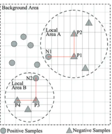
Fig. 2. An illustration of learning local influential regions. The distance between the adjacent vertical/horizontal grids is one unit. The location and radius of a local area could be learned and a suitable local metric could help to enhance the separability of the data, such as increasing l(N1P1)andl(N2P3)while decreasingl(P1P2)andl(P3P4).

each influential region improves class separability, as shown in Fig. 2.

To establish our new distance and local metric learning method, we first define some key concepts, namely influential regions, local metrics and line segments, which lead to the definition of the new distance. Then we calculate the distance by discussing the geometric relationship between line segment and influential regions. After that, we use the proposed local metric to build a novel classifier and study its learnability. The penalty terms from the derived learning bound, together with the empirical hinge loss, form an optimization problem, which is solved via gradient descent due to the non-convexity. Finally we experiment the proposed local metric learning algorithm on 20 publicly available data sets. On ten of these data sets, the proposed algorithm achieves the best performance, much better than the state-of-the-art metric learning competitors.

2 D

EFINITIONS OF

I

NFLUENTIAL

R

EGIONS

, L

OCAL

M

ETRICS AND

D

ISTANCE

In this section, we will first define influential regions As, s =

1, . . . , S, and the background region B. With a local metric for each region M(As) and M(B), the distance between xi and

xj will be defined as the sum of lengths of line segments in each influential region and the background region, as illustrated in Fig. 1. Since the metric is defined with respect to line segments, the distance is symmetric, i.e.D(xi,xj) =DM(xixj)(xi,xj) =

DM(xjxi)(xj,xi) =D(xj,xi).

To simplify the calculation required later, we restrict the shape of each influential region to be a ball.

Definition 1. Influential regionsare defined to be any set of balls or hyperspheres inside the metric space:

A={As, s= 1, . . . , S},

where S denotes the number of influential regions; As = Ball(os, rs), a ball with the center os and radius rs. Points

x₂Asconstruct a set with the following form:

{x|(os x)T(os x)rs2}. (1) The location of each influential region is determined by using the Euclidean distance.

Definition 2. Background region is defined to be the region excluding influential regions:

B=U [

s=1,...,S

As, whereU denotes the universe set.

Throughout this paper, the distance between two points xi and xj is equivalent to the length of line segment xixj, i.e.

D(xi,xj) =l(xixj). Lengthl(xixj)in influential regions and the background region will be defined separately with respective metrics.

Definition 3. Each influential regionAshas its ownlocal metric

M(As). The length of a line segmentxixj inside an influential regionAsis defined as1

l(xixj;M(As)) =DM(As)(xi,xj)

=q(xi xj)TM(As)(xi xj). (2) Here, we adopt the Mahalanobis distance, rather than the widely used squared Mahalanobis distance, since it simplifies the later optimization problem.

Definition 4. The background regionBhas abackground metric

M(B). For any two pointsxi,xj 2Bandxixj✓B, the length of a line segment is defined as

l(xixj;M(B)) = DM(B)(xi,xj)

= q(xi xj)TM(B)(xi xj). Note that for xi,xj 2 B and xixj * B, the distance betweenxiandxjis usually different fromDM(B)(xi,xj). This is because some parts of xixj may lie in influential regions so their lengths should be calculated via the related local metrics.

For any xi 2 U and xj 2 U, its line segment xixj may intersect with multiple influential regions and the background region. Therefore, we calculate the distance betweenxiandxjas the sum of lengths of line segments in each region. More precisely, as defined below, the distance is the sum of lengths of intersection ofxixj and influential regions, plus the length of intersection of

xixjand the background region.

Definition 5. Thelength of intersection of a line segmentxixj and an influential regionAsis defined asl(As\xixj;M(As)), where \ denotes the intersection operator. The length of the intersectionof a line segment xixj and the background region

Bis defined as l(B_\xixj;M(B)) =l(xixj [ s=1...S (As\xixj);M(B)) =l(xixj;M(B)) l( [ s=1...S (As\xixj);M(B)), (3)

whereS_s=1...S(A_s\xixj)denotes the union of intersections between the line segment and all influential regions.

Definition 6. Thelength of line segmentxixjis defined as

l(xixj;M(xixj)) =q(xi xj)TM(xixj)(xi xj) =l(B\xixj;M(B)) + X s l(As\xixj;M(As)), (4)

1. Since influential regions are restricted to be ball-shaped and a ball is a convex set,xixjwould lie in the ball for anyxiandxjinside the ball.

Fig. 3. The positions of u,v (intersection points between linexixj and the influential regionA) andp,q(intersection points between line

segmentxixjandA) under different situations.his the middle point of line segmentpq.

whereM(xixj)is the metric of the line segmentxixj.M(xixj) will be simplified asMafterwards.

3 C

ALCULATION OF

D

ISTANCES

3.1 Calculation of the Length of Intersection with Influ-ential Regions

We start by providing an intuitive explanation of calculating the length of intersection with influential regions, as illustrated in Fig. 3. If the line xixj does not intersect with (Fig. 3.1) or is the tangent to the influential ball (Fig. 3.2), the length is zero. If the line intersects with the ball (Fig. 3.3-3.8), we will calculate the length by considering the relationship between the intersection of the linexixj and the influential ball, i.e.uv, and the intersection of the line segmentxixjand the influential ball, i.e.pq.

First, we show that the length of intersection can be calculated given the local metricM(As)and the intersection ratio defined below.

Definition 7. The intersection points of the line xixj and the influential regionAs are represented asu =xi+ u(xj xi) and v = xi + v(xj xi), where u, v 2 R, u  v, and u, vare called theintersection coefficientsbetween the line

xixj andAs. Theintersection pointsof the line segment xixj and the influential region are represented asp=xi+ p(xj xi) andq=xi+ q(xj xi), where0 p q1and p, q are called theintersection coefficients between the line segment

xixjandAs. = q pis called theintersection ratio. Proposition 1. The length of intersection between line segment

xixj and the influential regionAs, with the intersection points

p,qand intersection coefficients p, q, is

l(A_\xixj;M(As)) = q (q p)T_M(A s)(q p) = q(xi xj)TM(As)(xi xj). (5) Next, we figure out the relationship between the line xixj and the influential ball via the one-variable quadratic equation and

TABLE 1

Relationship between u, vand p, qfor different positions ofxixj

Illustration u, p v, q Fig. 3.3 u<0) p= 0 v<0) q= 0 Fig. 3.4 u>1) p= 1 v>1) q= 1 Fig. 3.5 u<0) p= 0 v>1) q= 1 Fig. 3.6 0 u1) p= u 0 v1) q= v Fig. 3.7 0 u1) p= u v>1) q= 1 Fig. 3.8 u<0) p= 0 0 v1) q= v

calculate u, v when they exist. xixj intersects withAsif we can findu,vthat lie on the surface of the ball, which is equivalent to solving the following quadratic equation in one variable :

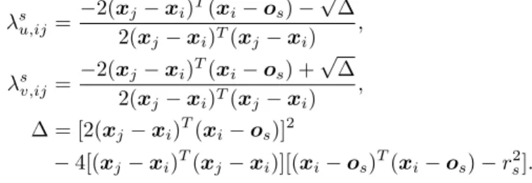
kxi+ (xj xi) osk22=r2s. (6) If the discriminant of (6) is positive, then u,v exist and the solutions s

u,ij  sv,ij are given by the quadratic equation s u,ij = 2(xj xi)T(xi os) p 2(xj xi)T(xj xi) , s v,ij = 2(xj xi)T(xi os) + p 2(xj xi)T(xj xi) , = [2(xj xi)T(xi os)]2 4[(xj xi)T(xj xi)][(xi os)T(xi os) r2s]. For simplicity, we will drop the superscriptsand subscriptij.

Last, we calculate q, p based on u, v. Since0 p  q  1, we set p = u if and only if u 2 [0,1] and similarly for q. In other words, we set u, v as follows: p = min(max( u,0),1), q = min(max( v,0),1). Details are given in Table 1.

3.2 Calculation of the Length of Intersection Using Lo-cal Metrics

Proposition 2. In the case of non-overlapping influential regions, i.e.Ai\Aj =;,8i6=j, DM(xi,xj) = b q (xi xj)TM(B)(xi xj) +X s s q (xi xj)TM(As)(xi xj), (7) where b is defined as the intersection ratio of the background region and b= 1 Ps s. Proof: DM(xi,xj) =l(xixj;M(B)) l( [ s=1...S (As\xixj);M(B)) +X s l(As\xixj;M(As)) = (1 X s s) q (xi xj)TM(B)(xi xj) +X s s q (xi xj)TM(As)(xi xj).

Proposition 2 suggests that the distance can be obtained given metrics (M(As),M(B)) and the intersection ratio s. All calcu-lations are in closed form and hence the computation is efficient.

To avoid creating overlapping influential regions, we will conduct overlap detection during parameter updates. If the update

of location parameters (o, r) leads to overlap, then we will skip this update and continue on learning other parameters.

4 C

LASSIFIER AND

L

EARNABILITY

In this paper, we select Lipschitz continuous functions as our classifiers since they are a family of smooth functions which are learnable [24]. Based on the resultant learning bounds, we obtain the regularization terms in order to improve the classifier’s generalization ability.

4.1 Classifier

To start with, we can see that the following classifier gives the same classification result as 1-NN:

f(x) = minDset(x,X ) minDset(x,X+), where Dset(x,X /+) = {D(x,xt)|8xt 2 negative class / positive class} andD(xi,xj) denotes the distance betweenxi andxjdefined by any metric.f(x)<0indicates thatxbelongs to negative class andf(x)>0indicates thatxbelongs to positive class.

In this paper, in order to achieve robustness to noisy instances and incorporate more flexible distance metrics, we extend the above equation by considering more nearby instances as follows:

f(x) =1 K K X k=1 D_[k](x,X ) 1 K K X k=1 D_[k](x,X+_{), (8)}

whereD_[k](x,X) =_{D(x,xt)|8xt 2 X}[k] denotes the kth

smallest element of the distance set{D(x,xt)|8xt 2X}. This function will be used as the classifier in our algorithm.

For multiclass classification, the result will be given by

y = argmin_c

K X k=1

D_[k](x,Xc_),

whereXc denotes the training instances of class c. It gives the same classification result as (8) in the binary case.

4.2 Learnability of the Classifier with Local Metrics We will discuss learnability of functions based on the Lipschitz constant, which characterizes the smoothness of a function. The smaller the Lipschitz constant is, the smoother the function is. Definition 8. [25] Let(_X,⇢_X),(_Y,⇢_Y)be two metric spaces. TheLipschitz constantof a functionf is

Lip(f) = min{C2R_{|8xi,xj 2X,xi6=xj,} ⇢_Y(f(xi), f(xj))C⇢X(xi,xj)} = max xi,xj2X:xi6=xj ⇢_Y(f(xi), f(xj)) ⇢_X(xi,xj) .

Proposition 3. [25] LetLip(f)_Lf andLip(g)Lg, then (a)Lip(f+g)_Lf+Lg;

(b)Lip(f g)Lf+Lg;

(c)Lip(af)_|a_|Lf, whereais a constant.

Proposition 4. Let Lip(fk(x))  L, k = 1, . . . , N, then, for any K  N, Lip(PK_k=1f[k](x)) is bounded by KmaxkL, where f[k](x) denotes the kth smallest element of the set {fk(x), k= 1, . . . , K}. Proof. ₈xi,xj 2X, k2{1, . . . , N} K X k=1 f[k](xi) = K X k=1 {fk(xj) +fk(xj+ (xi xj)) fk(xj)}[k]  K X k=1 {fk(xj) +Lkxj+ (xi xj) xjk}[k]  K X k=1 {fk(xj) +Lkxi xjk}[k] = K X k=1 f[k](xj) +KLkxi xjk.

Based on the definition of Lipschitz constant, the proposition is proved.

Lemma 1. With distance defined in (7), the Lipschitz con-stant of the classifier specified in (8) is bounded by L = 2(P_spkM(As)kF+

p

kM(B)kF), wherek·kF denotes the matrix Frobenius norm.

Proof. Let dM(x,xk) denote the Mahalanobis distance with metricM, i.e.

dM(x,xk) = q

(x xk)TM(x xk),

and dI(x,xk) denotes the Euclidean distance with the identity matrixI.

The Mahalanobis distancedM(x,xk)has the Lipschitz con-stant ofpkM_kF as follows: Lip(dM(x,xk)) = sup xa,xb2X,xa6=xb dM(xa,xk) dM(xb,xk) dI(xa,xb)  sup xa,xb2X,xa6=xb dM(xa,xb) dI(xa,xb)  sup xa,xb2X,xa6=xb dI(xa,xb) p kM_kF dI(xa,xb) =q_kM_kF,

where the first inequality follows the triangle inequality of dis-tance, and the second inequality is based on the Cauchy-Schwarz inequality and the fact that Frobenius norm is compatible with the vectorl2norm.

According to the definition of distance in (7), we have

DM(x,xk) = X s sdM(As)(x,xk) + bdM(B)(x,xk) X s dM(As)(x,xk) +dM(B)(x,xk)

as s, b1. From Proposition 3, we get that

Lip(DM(x,xk)) X s q kM(As)kF+ q kM(B)_kF.

Based on the Lipschitz constant ofDM(x,xk)and the com-position property illustrated in Procom-position 4,

Lip( K X k=1 {DM(x,xk), k= 1, . . . K}[k]) K ( X s q kM(As)kF + q kM(B)kF ) .

Finally, based on Proposition 3, f(x) in (8) is bounded by

2(P_spkM(As)kF+ p

kM(B)kF).

Combining Lemma 1 and Corollary 2 of [24], we can obtain the following Corollary.

Corollary 1. Let metric space X have doubling dimension

ddim(_X)and letFbe the collection of real valued functions over

Xwith the Lipschitz constant at mostL. Then for anyf _2Fthat classify correctly on all butkexamples, we have with probability at least1 P_{(x, t) : sign[f(x)]₆=t_} k_n+ r 2 n(cln(34en/c) log2(578n) + ln(4/ )), (9) wherendenotes the sample size,t_2{ 1,1_}denotes the label, and c(16Ldiam(X))ddim(X) =⇣32(X s q kM(As)kF + q kM(B)_kF) diam(_X)⌘ddim(X).

diam denotes the diameter of the space and ddim denotes doubling dimension; precise definitions can be found in [24].

The above learning bound illustrates that the generalization ability, i.e. the difference between the expected errorP_{(x, t) : sign[f(x)] 6= t}and the empirical errork/n, can be improved by reducing the value of P_spkM(As)kF +

p

kM(B)_kF. Since the square function is monotonically increasing, we would instead reduce PskM(As)kF +kM(B)kF. In other words, P

skM(As)kF+kM(B)kFwould be used as the regularization term to improve the generalization ability of the classifier.

5 O

PTIMIZATION

P

ROBLEM

5.1 Objective Function

In order to obtain low training error and good generalization ability, we propose the following optimization problem, where the objective function consists of a sum of hinge loss and the regularization termP_skM(As)kF+kM(B)kF: min ⇥,⇠ 1 N1 X (i,j) ⇠ij+ 1 N2 X (m,n) ⇠mn+↵ X s kM(As)kF +↵kM(B)kF s.t.DM(xi,xj)1 C+⇠ij, DM(xm,xn) 1 +C+⇠mn ⇠ij,⇠mn 0, M2M+ i, m= 1, . . . , N, j _!i, n9m, (10) where⇥=_{M(As), M(B),o,r}denotes the set of parameters to be optimized;j !idenotes thatxjisxi’sKnearest neighbor comparing against all instances in the same class; m 9 n

denotes thatxn isxm’sK nearest neighbor comparing against all instances in the different class;C is a constant which has the intuition of margin;⇠ijand⇠mndenote the error caused by margin violation;N, N1, N2denote the number of training samples, pairs

(i, j), and pairs(m, n) respectively ;↵is a trade-off parameter between the margin loss and the regularization terms. This opti-mization formula is suitable for both binary and multi-class tasks. In the proposed algorithm, we will learn the locations of influential regions (os, rs) and the metrics of influential/background regions (M(B), M(As)) under the same framework.

5.2 Gradient Descent

WithDM(As) andDM(B)being the Mahalanobis distances, the

optimization problem is convex even wheno,rare fixed and only

M(As)andM(B)are updated. Therefore, we adopt the gradient descent algorithm:

⇥t+1=⇥t @g

@⇥|⇥t,

where is the learning rate, and the superscripttdenotes the time step during optimization.

The objective functiongis

g= 1 N1[DM(xi,xj) (1 C)]++↵ X s kM(As)kF + 1 N2 [1 +C DM(xm,xn)]++↵kM(B)kF,

where the distance is

DM(xi,xj) = [ b(os, rs)]+DM(B)(xi,xj)

+ X

s

s(os, rs)DM(As)(xi,xj)

and b(os, rs) = 1 Ps s(os, rs). Here, s is written as s(os, rs) to remind us that s is a function of the location parametersosandrs.

The gradient ofgwith respect to parameterso, ris

@g @⇥|⇥t = 1 N1 X (i,j) 1[DMt(x_i,x_j) (1 C)>0]@DM(xi,xj) @⇥ |⇥t 1 N2 X (m,n) 1[1 +C DMt(x_m,x_n)>0] @DM(xm,xn) @⇥ |⇥t.

If the gradient is with respect to M(B) and M(As_{), then the} shrinkage term of ↵M(B)

kM(B)k or

↵M(As)

kM(As)k should be added into the

above formula.

Now we will calculate @DM(xi,xj)

@⇥ |⇥t for the parameters

M(As),M(B),os,rsseparately: @D(xi,xj) @M(As) |⇥ t = s(o t s, rts) 2 ⇥ [(xi xj)TMt(As)(xi xj)] 1/2(xi xj)(xi xj)T; @D(xi,xj) @M(B) |⇥t = 1[ b(ots, rst)>0] b(ots, rst) 2 ⇥ [(xi xj)TMt(B)(xi xj)] 1/2(xi xj)(xi xj)T; @D(xi,xj) @os |⇥ t = @ s @os D_Mt_(As)(x_i,x_j) @ s @os 1[ b(ots, rts)>0]DMt_(B)(x_i,x_j) where@

@o could be obtained as illustrated in Table 2;

@D(xi,xj) @rs |⇥ t =@ s @rs DMt_(A s)(xi,xj) @ s @rs 1[ b(ots, rts)>0]DMt_(B)(x_i,x_j), where@

@r could be obtained as illustrated in Table 2.

Initial values are crucial for non-convex optimization prob-lems. We adopt a heuristic method to initialize the parameters as

TABLE 2 Partial gradients of@ @o and @ @r in different cases. !

oh,!ov,ou!can be found from Fig. 3.

u, v partial gradients u<0, v<0 0 u<0, v>1 1 _@@_o =0,@_@r = 0 u>1, v>1 0 0 u1,0 v1 v u @_@o= 2 1/2_(x j xi)T(xi o)(xj xi) (xj xi)T(xj xi) 4 1/2_{(o x} i) = 4 1/2oh,! @_@r = 4 1/2r u<0,0 v1 v @_@o =(xj xi) 1/2_(x j xi)T(xi o)(xj xi) (xj xi)T(xj xi) 2 1/2_{(o x} i) = 2 1/2!ov, @_@r = 2 1/2r 0 u1, v>1 1 u @_@o = (xj xi) 1/2_(x j xi)T(xi o)(xj xi) (xj xi)T(xj xi) 2 1/2_{(o x} i) = 4 1/2ou,! @_@r = 2 1/2r

follows. 1) Extract local discriminative directionh(x)₂RF _for each training instancex, whereFindicates the number of features ofx: h(xi)[f] = X k9i |xk[f] xi[f]| X j!i |xj[f] xi[f]|, wherex[f]indicates thefth dimension of vector x. 2) Perform nonparametric clustering: The Dirichlet process Gaussian mixture model is applied to the augmented feature vector [x, h(x)] to group instances into clusters; the number of clusters, and hence the number of influential regions, is automatically decided by the clustering algorithm. 3) Initialize the parameters: Cluster centers are initialized asos; the80th percentile of the distance between samples and the cluster center is set as initial value of rs; the local metric is set asM(As) =I+ 0.1⇥diag(mean(h(x),x2 clusters)), where diag is an operation which returns a square diagonal matrix with elements of the input vector on the main diagonal. The initialization process is carried out from the largest cluster to the smallest one. If a later influential region overlaps with an earlier one, the later region will be shrunk, or even deleted, until no overlap exists.

6 E

XPERIMENTS

6.1 Toy Example

To visualize the learned parameters, we consider a toy data set for binary classification consisting of 80 instances generated from a two-component Gaussian mixture model. 40 instances in the positive and 40 instances in the negative class are sampled from1

2N[( 1,0),12I]+12N[(1,0),12I]and 12N[( 1,2),12I]+ 1

2N[(3,0),12I]respectively. Parameters in our algorithm are set

as follows: ↵ and C in the optimization formula are 0.1 and

0.5 respectively; the number of clusters used for initializing the parameters is 2; the gradient descent algorithm stops after 50 iterations. For illustration purpose, overlap detection has not been conducted on the toy example.

In Figs. 4a-4c, we learn one parameter from {M(A),o, r}

at each time, fixing the other parameters. Take Fig. 4a (left) as an example. SinceM(A1) = M(A2) = 2I and M(B) = I,

the influential regions act as enlarging the local distance. In this case, we see that the centers ofA1and A2move to the inter-class region. This phenomenon could be explained as follows. For a line segment that lies in an inter-class region and vio-lates the margin constraint, i.e. DM(xm,xn) < 1 +C, the direction of gradient descent is same as that of @DM(xm,xn)

@o .

AsDM(A)(xm,xn) > DM(B)(xm,xn), @DM(_@x_om,xn) has the same direction as @r

@o, which, according to Table 2, is the direction

of oh!, ou!, !ov in Fig. 3 depending on the value of . In other words, the margin-violated inter-class line segments will pull the influential regions towards the inter-class region. At the same time, for an intra-class line segment that violates the margin constraint, i.e. DM(xi,xj) > 1 C, the direction of gradient descent is opposite to that of @DM(xm,xn)

@o , and hence opposite to

!

oh, !

ou,!ov. That is, the margin-violated intra-class line segments will push the influential regions away from the intra-class region. In summary, as illustrated in Fig. 4a (left), when the influential regions have the effect of ‘enlarging’ distance, o move to the inter-class region. Similar reasoning applies to Fig. 4a (right), 4b, and 4c. In Fig. 4d, M(A),o, r are learned simultaneously. As expected, the influential regions focus on inter-class samples by moving towards the inter-class region, increasing the region size, and enlarging the local distance in the direction that is nearly perpendicular to the decision boundary.

The toy example demonstrates that the gradient learning has a clear geometric interpretation.

6.2 Real Data

We compare our algorithm with twelve established metric learn-ing algorithms from three categories: (1) the most cited algo-rithms, including large margin nearest neighbor (LMNN) [2] and information theoretic metric learning (ITML) [3]; (2) lo-cal metric learning algorithms, including multiple-metric large margin nearest neighbor (mmLMNN) [2], parametric local met-ric learning (PLML) [17], reduced-rank local distance metmet-ric learning (R2LML) [18], and local discriminative distance met-rics ensemble learning (LDDM) [26]; (3) the state-of-the-art metric learning algorithms, including distance metric learning with eigenvalue optimization (DMLE) [27], sparse compositional metric learning (SCML) [20], stochastic neighbor compression (SNC) [28], regressive virtual metric learning (RVML) [29], geometric mean metric learning (GMML) [30], and supervised distance metric learning through maximization of the Jeffrey divergence (DMLMJ) [31]. LMNN and ITML are implemented using the metric-learn toolbox2_{; mmLMNN, PLML, R2LML,} LDDM, DMLE, SCML, SNC, RVML, GMML and DMLMJ are implemented using the authors’ code.

We conduct binary classification on 14 data sets and multiple-class multiple-classification on 6 data sets, all of which are publicly available from UCI3 _{and LibSVM}4_{. For binary classification,} we use data sets Australian, Breastcancer, Diabetes, Fourclass,

2. https://all-umass.github.io/metric-learn/ 3. https://archive.ics.uci.edu/ml/datasets.html

TABLE 3

Metric learning algorithm results: Mean accuracy and standard deviation are reported with the best ones in bold; ‘AVERAGE’ denotes the average accuracy of all data sets; ‘#of BEST’ denotes the number of data sets that an algorithm performs the best; ‘NAN’ indicates the algorithm cannot

return a classification result for the data set.

Data sets LMNN ITML mmLMNN PLML R2LML LDDM DMLE SCML SNC RVML GMML DMLMJ LMLIR Binary classification Australian 78.8±2.6 77.2±1.9 82.5±2.6 80.5±1.1 84.7±1.3 72.8±9.1 82.6±1.5 82.3±1.4 81.8±8.8 83.0±1.6 84.4±1.0 83.9±1.3 85.1±1.9 Breastcancer 95.9±0.7 96.4±1.0 96.7±1.0 96.4±0.9 97.0±0.7 66.1±1.8 97.0±1.1 97.0±0.9 96.7±0.7 95.8±1.1 97.3±0.8 96.6±0.8 96.4±2.1 Diabetes 69.2±1.4 69.1±1.2 72.2±1.9 68.5±2.0 73.8±1.4 64.4±2.0 72.6±2.0 71.5±2.2 75.3±2.7 71.0±2.6 74.2±2.6 71.5±3.1 75.9±1.9 Fourclass 72.1±2.3 72.1±2.2 75.6±1.4 72.4±2.4 76.1±1.9 64.0±2.1 75.6±1.4 75.5±1.4 73.4±8.7 70.5±1.4 76.1±1.9 76.1±1.9 79.9±0.9 German 67.9±1.5 67.0±2.1 68.9±1.8 70.0±2.9 72.9±1.8 70.1±1.5 72.0±2.1 70.9±2.7 70.1±3.3 71.7±1.8 71.6±1.1 69.3±2.7 73.7±1.6 Haberman 67.9±3.3 68.0±4.1 69.0±2.7 67.1±3.1 71.1±3.4 73.8±3.6 70.8±3.5 69.2±2.5 72.0±5.2 66.7±2.3 71.2±3.4 68.5±3.2 74.4±3.7 Heart 76.2±3.8 76.9±3.3 79.4±3.7 75.1±3.2 82.0±3.8 71.6±9.7 77.9±3.1 79.0±3.2 77.0±5.3 77.7±4.1 81.2±2.7 80.6±2.8 83.1±3.2 ILPD 67.0±2.1 68.7±2.8 66.8±2.1 67.4±3.0 65.9±2.2 72.4±1.1 68.8±2.7 68.0±2.9 68.9±2.7 68.0±2.9 67.1±2.2 68.0±1.6 69.6±2.7 Liverdisorders 61.0±4.8 57.2±4.0 62.0±3.5 62.2±2.5 66.8±3.7 56.8±3.8 61.8±2.7 61.7±4.6 63.3±5.2 64.6±3.9 63.8±5.4 60.9±3.8 66.7±3.6 Monk1 88.4±2.6 77.3±1.3 90.3±2.6 96.6±2.7 89.2±1.5 67.9±8.1 99.9±0.3 97.5±0.9 96.8±4.8 89.2±2.7 75.0±2.6 87.7±3.8 95.0±7.2 Pima 68.5±1.6 68.0±2.0 72.5±2.7 68.4±2.2 72.3±1.5 64.9±2.6 72.1±2.4 71.1±2.6 74.0±2.6 69.5±1.7 73.0±1.8 71.1±2.8 74.6±2.0 Planning 60.4±5.3 62.2±2.3 54.7±3.4 60.8±5.5 63.9±3.4 72.1±7.8 60.1±5.5 61.9±5.0 NAN 55.1±7.4 65.2±5.5 64.3±2.9 67.5±6.5 Voting 94.8±0.8 90.8±1.4 95.4±0.9 95.5±1.0 96.3±1.2 65.1±10.3 93.1±1.9 95.0±1.3 94.5±1.2 95.8±1.3 95.2±1.9 95.3±1.1 93.2±3.9 WDBC 96.6±1.1 94.9±0.9 97.4±1.0 96.4±0.9 96.9±1.7 63.2±3.5 96.7±0.5 97.0±0.9 96.9±0.9 96.6±1.3 96.7±0.8 97.3±1.9 96.6±1.0 AVERAGE 76.0 74.6 77.3 76.9 79.2 67.5 78.6 78.4 NAN 76.7 77.9 77.9 80.8 #of BEST 0 0 1 0 2 2 1 0 0 0 1 0 7 Multiclass classification Cleveland 54.6±2.1 56.2±2.2 53.9±2.2 49.0±4.1 57.7±2.1 52.9±2.3 54.0±2.4 54.4±3.5 53.3±3.1 50.9±4.4 59.1±2.3 55.3±3.2 57.7±3.5 Glass 70.7±4.8 69.9±4.7 NAN NAN 70.2±5.5 41.6±9.0 66.2±5.3 71.7±2.9 69.5±6.5 68.1±3.7 69.9±6.0 59.3±5.1 72.0±5.7 Iris 86.7±2.9 87.0±3.3 86.5±3.6 82.7±6.9 87.0±4.6 70.0±13.3 86.8±3.6 87.3±3.1 NAN 83.8±4.2 87.5±3.7 85.3±4.8 87.8±3.8 Newthyroid 88.6±2.7 90.0±2.3 88.5±3.2 89.0±2.1 90.4±3.2 69.9±3.0 89.2±2.1 89.3±3.3 89.7±2.5 88.3±1.8 89.8±3.4 91.1±2.1 90.6±1.9 Tae 50.2±8.2 46.2±7.0 50.2±7.2 50.8±8.3 50.8±6.1 29.2±5.1 49.7±4.4 53.6±5.9 NAN 55.4±6.9 51.2±6.3 49.0±6.9 53.6±6.7 Winequality(red) 58.3±1.9 56.1±1.5 NAN NAN 58.0±1.2 NAN 55.0±1.7 58.9±1.7 58.2±4.0 59.6±2.3 58.2±1.8 49.0±3.9 60.08±6.5

AVERAGE 73.0 71.8 NAN NAN 75.2 62.1 74.1 75.1 NAN 73.8 74.3 72.7 76.9

#of BEST 0 0 0 0 0 0 0 0 0 1 1 1 3

Germannumber, Haberman, Heart, ILPD, Liverdisorders, Monk1, Pima, Planning, Voting, and WDBC; for multiple-class, we use Cleveland, Glass, IRIS, Newthyroid, Tae, and Winequality (red). All data sets are pre-processed by firstly subtracting the mean and dividing by the standard deviation, and then normalizing the L2-norm of each instance to one.

For each data set, 60% instances are randomly selected as training samples and the rest for testing. This process is repeated 10 times and the mean accuracy and the stan-dard deviation are reported. We use 10-fold cross-validation to select the trade-off parameters in the compared algo-rithms, namely the regularization parameter of LMNN (from

{0.1,0.3,0.5,0.7,0.9_}), in ITML (from{0.25,0.5,1,2,4_}),t

in GMML (from{0.1,0.3,0.5,0.7,0.9}) and in RVML (from

{10 5_,10 4_{, . . . ,10}). All other parameters are set as default.}

For our algorithm, we set the parameters as follows:↵andC in the optimization formula are0.1and0.5respectively;K in the classifier is10. The number of influential regions in our algorithm is determined via Dirichlet process Gaussian mixture model and it is implemented with PRML toolbox5_.

Results for binary classification and multiclass classification are shown in Table 3. The proposed algorithm achieves the highest average accuracy on both tasks. Out of 20 data sets, LMLIR outperforms all other methods on ten data sets out and none of the other algorithms performs the best in more than two data sets. In cases where our algorithm is not leading, the difference to the optimal method is relatively small. Such encouraging results demonstrate the effectiveness of our proposed method.

7 C

ONCLUSIONS AND FUTURE WORK

In this short paper, by introducing influential regions, we define a very intuitive distance and propose a novel local metric learning method. The distance can be computed efficiently and encouraging results are obtained on public data sets.

5. https://github.com/PRML/PRMLT

Some directions merit future investigation to extend our work. Original features from data are used in this paper, but we may explore deep features for specified tasks. More advanced optimiza-tion techniques and other types of influential regions may also be explored. Domain knowledge can be embedded into the partition of the regions. Tighter learning bounds and resultant penalty terms would also be our future work.

R

EFERENCES

[1] E. P. Xing, M. I. Jordan, S. Russell, and A. Y. Ng, “Distance metric learn-ing with application to clusterlearn-ing with side-information,” inAdvances in neural information processing systems, 2002, pp. 505–512.

[2] K. Q. Weinberger and L. K. Saul, “Distance metric learning for large margin nearest neighbor classification,”The Journal of Machine Learn-ing Research, vol. 10, pp. 207–244, 2009.

[3] J. V. Davis, B. Kulis, P. Jain, S. Sra, and I. S. Dhillon, “Information-theoretic metric learning,” in Proceedings of the 24th international conference on Machine learning. ACM, 2007, pp. 209–216.

[4] R. Jin, S. Wang, and Y. Zhou, “Regularized distance metric learning: Theory and algorithm,” in Advances in neural information processing systems, 2009, pp. 862–870.

[5] Z.-C. Guo and Y. Ying, “Guaranteed classification via regularized simi-larity learning,”Neural computation, vol. 26, no. 3, pp. 497–522, 2014. [6] Q. Cao, Z.-C. Guo, and Y. Ying, “Generalization bounds for metric and

similarity learning,”Machine Learning, vol. 102, no. 1, pp. 115–132, 2016.

[7] N. Verma and K. Branson, “Sample complexity of learning mahalanobis distance metrics,” inAdvances in Neural Information Processing Sys-tems, 2015, pp. 2584–2592.

[8] J. Hu, J. Lu, and Y.-P. Tan, “Discriminative deep metric learning for face verification in the wild,” inProceedings of the IEEE Conference on Computer Vision and Pattern Recognition, 2014, pp. 1875–1882. [9] J. Lu, G. Wang, W. Deng, P. Moulin, and J. Zhou, “Multi-manifold

deep metric learning for image set classification,” inProceedings of the IEEE Conference on Computer Vision and Pattern Recognition, 2015, pp. 1137–1145.

[10] W. Liu, D. Xu, I. Tsang, and W. Zhang, “Metric learning for multi-output tasks,”IEEE Transactions on Pattern Analysis and Machine Intelligence, 2018.

[11] J. Hu, J. Lu, and Y.-P. Tan, “Sharable and individual multi-view metric learning,”IEEE transactions on pattern analysis and machine intelli-gence, 2017.

(a) Learn the centerso withM, r being fixed: when the

influential regions have the effect of ‘enlarging’ distance (left),omove to the inter-class region; when the influential regions have the effect of ‘shrinking’ distance (right), o

move to the intra-class region.

(b) Learn the radii r with M,o being fixed: when the

influential regions have the effectiveness of ‘enlarging’ dis-tance (left), the region lying in the intra-class region (i.e. A1) decreases its size and the region lying in inter-class region (i.e. A2) increases its size; when the influential re-gions have the effectiveness of ‘shrinking’ distance (right),

rA1increases andrA2decreases.

(c) Learn local metrics M(A1),M(A2) with o, r being

fixed: Starting from initial metrics2I(left), the metric that

is learned in the intra-class region shrinks its distance; the metric that is learned in the inter-class region enlarges the distance in the direction to the decision boundary (right).

(d) Learn o, r,M(A1),M(A2): Both influential regions

move towards the inter-class region and increase their sizes. The learned local metrics enlarge the distance be-tween samples from different classes.

Fig. 4. Illustration of parameter learning using a toy data set. This figure is best viewed in color.

[12] L. Yang, R. Jin, L. Mummert, R. Sukthankar, A. Goode, B. Zheng, S. C. Hoi, and M. Satyanarayanan, “A boosting framework for visuality-preserving distance metric learning and its application to medical image retrieval,”IEEE Transactions on Pattern Analysis and Machine Intelli-gence, vol. 32, no. 1, pp. 30–44, 2010.

[13] J. Lu, X. Zhou, Y.-P. Tan, Y. Shang, and J. Zhou, “Neighborhood repulsed metric learning for kinship verification,”IEEE transactions on pattern analysis and machine intelligence, vol. 36, no. 2, pp. 331–345, 2014. [14] Z. Huang, R. Wang, S. Shan, L. Van Gool, and X. Chen, “Cross

Euclidean-to-Riemannian metric learning with application to face recog-nition from video,”IEEE Transactions on Pattern Analysis and Machine Intelligence, 2017.

[15] B. Wang, G. Wang, K. L. Chan, and L. Wang, “Tracklet association by online target-specific metric learning and coherent dynamics estimation,”

IEEE transactions on pattern analysis and machine intelligence, vol. 39, no. 3, pp. 589–602, 2017.

[16] A. Frome, Y. Singer, F. Sha, and J. Malik, “Learning globally-consistent local distance functions for shape-based image retrieval and classifica-tion,” inComputer Vision, 2007. ICCV 2007. IEEE 11th International Conference on. IEEE, 2007, pp. 1–8.

[17] J. Wang, A. Kalousis, and A. Woznica, “Parametric local metric learning for nearest neighbor classification,” inAdvances in Neural Information Processing Systems, 2012, pp. 1601–1609.

[18] Y. Huang, C. Li, M. Georgiopoulos, and G. C. Anagnostopoulos, “Reduced-rank local distance metric learning,” inJoint European Con-ference on Machine Learning and Knowledge Discovery in Databases. Springer, 2013, pp. 224–239.

[19] J. Bohn´e, Y. Ying, S. Gentric, and M. Pontil, “Large margin local metric learning,” inEuropean Conference on Computer Vision. Springer, 2014, pp. 679–694.

[20] Y. Shi, A. Bellet, and F. Sha, “Sparse compositional metric learning,” in

AAAI, 2014, pp. 2078–2084.

[21] S. Saxena and J. Verbeek, “Coordinated local metric learning,” in

Proceedings of the IEEE International Conference on Computer Vision Workshops, 2015, pp. 127–135.

[22] J. St Amand and J. Huan, “Sparse compositional local metric learning,” inProceedings of the 23rd ACM SIGKDD International Conference on Knowledge Discovery and Data Mining. ACM, 2017, pp. 1097–1104. [23] Y. Noh, B. Zhang, and D. Lee, “Generative local metric learning for

nearest neighbor classification.”IEEE transactions on pattern analysis and machine intelligence, vol. 40, no. 1, p. 106, 2018.

[24] L.-A. Gottlieb, A. Kontorovich, and R. Krauthgamer, “Efficient clas-sification for metric data,”Information Theory, IEEE Transactions on, vol. 60, no. 9, pp. 5750–5759, 2014.

[25] N. Weaver and N. Weaver,Lipschitz algebras. World Scientific, 1999. [26] Y. Mu, W. Ding, and D. Tao, “Local discriminative distance metrics

ensemble learning,”Pattern Recognition, vol. 46, no. 8, pp. 2337–2349, 2013.

[27] Y. Ying and P. Li, “Distance metric learning with eigenvalue optimiza-tion,”Journal of Machine Learning Research, vol. 13, no. Jan, pp. 1–26, 2012.

[28] M. Kusner, S. Tyree, K. Weinberger, and K. Agrawal, “Stochastic neigh-bor compression,” inInternational Conference on Machine Learning, 2014, pp. 622–630.

[29] M. Perrot and A. Habrard, “Regressive virtual metric learning,” in

Advances in Neural Information Processing Systems, 2015, pp. 1810– 1818.

[30] P. Zadeh, R. Hosseini, and S. Sra, “Geometric mean metric learning,” in

International Conference on Machine Learning, 2016, pp. 2464–2471. [31] B. Nguyen, C. Morell, and B. De Baets, “Supervised distance metric

learning through maximization of the jeffrey divergence,”Pattern Recog-nition, vol. 64, pp. 215–225, 2017.