TIME SERIES MODELING FOR FORECASTING WHEAT PRODUCTION
OF PAKISTAN
M. Amin, M. Amanullah and A. Akbar
Department of Statistics Bahauddin Zakariya University, Multan, Pakistan. Corresponding Author E mail: [email protected]
ABSTRACT
Wheat is the main agriculture crop of Pakistan. For country planning, forecasting is the main tool for predicting the production of wheat to determine the situation what would be the value of production coming year. In this research, we developed time series models and best model is identified for the objective to forecast the wheat production of Pakistan. In this research large time periods i.e. 1902-2005 data was used. Various time series models are fitted on this data using two software’s JMP and Statgraphics. We have found that the best model is ARIMA (1, 2, 2). On the basis of this selected model, we have found that wheat production of Pakistan would become 26623.5 thousand tons in 2020 and would become double in 2060 as compared in 2010.
Key words: ARIMA; Time Series models; Wheat Production Forecasting.
INTRODUCTION
Agriculture is the backbone of Pakistan’s economy and it contributes to the economic and social well being of the nation through its influence on the gross domestic product (GDP), employment and foreign exchange earnings. In food grain crops, wheat and rice are the most important in the agriculture sector, in that rice contributes 5.4% of value added in agriculture and 1.3% to GDP and wheat accounts for 13.8% in value added in agriculture and 3.4% in GDP (Government of Pakistan, 2004). Agriculture plays an important role in the betterment of the large proportion of the rural population in particular and overall economy in general. Agricultural development is desired in almost every part of the world today. The race between increasing population and food supply is a real grim. Wheat is the main staple food for the people of Pakistan. The unprecedented drought and water shortage conditions have severely affected the wheat crop during the last years.
Wheat production forecasting is mainly depends on the cultivated area. Therefore it is necessary to develop the model for, to determine the estimated wheat production on the basis of cultivated area in the long run. Many studies have been conducted to forecast and determine constraints in the production of major crops such as wheat, cotton and rice in Pakistan. Despite these constraints, there are indeed good prospects for continued growth in the area and yield of wheat and other crops in Pakistan (Hamid et al., 1987; Muhammad, 1989). Qureshi et al. (1992) analyzed the relative contribution of area and yield to total production of wheat and maize in Pakistan and concluded that there was more than 100% increase in total wheat production that can be attributed
to yield enhancement. Muhammad et al. (1992) conducted an empirical study of modeling and forecasting time series data of rice production in Pakistan. ARIMA model has been frequently employed to forecast the future requirements in terms of internal consumption and export to adopt appropriate measures (Muhammad et al., 1992; Shabur and Haque, 1993; Sohail et al., 1994).
Factually, other crops in general and wheat in particular provide linkages through which it can stimulate economic growth in other sectors. Wheat cultivation has been suffering from various problems, such as traditional methods of farming, low yields, shortage of key inputs and shortage of irrigation water. Pakistan has experienced ups and downs in wheat production. Prices of wheat and flour boosts up during low production seasons and falls drastically when there is a surplus wheat production, however, surplus wheat production occurred for few years and during such periods farming community suffered heavy losses due to inadequate marketing facilities in the country. On the other hand, farmers do not know future prospect of wheat production and prices while deciding to cultivate this and other crops. There is a dire need to forecast area, yield and production of wheat in Pakistan. Therefore, the objective of this paper is to determine future prospects of wheat in the country using past trends.
Karim et al. (2005) applied regression modeling to forecast wheat production of Bangladesh districts. They usedseven model selection criteria’s and found that different models were identified for different districts for wheat production forecasts. They have found that wheat production in Bangladesh districts i.e. Dinajpur, Rajshahi, and Rangpur would be 1.54, 0.35, 0.31, and 0.58 million tons, respectively, in 2009/10. Iqbal et al. (2000) used
ARIMA model for forecasting wheat area and production in Pakistan. They used ARIMA (1,1,1) model for wheat area forecasting and ARIMA(2,1,2) model for wheat production forecasting. They have found that for 2000-2001 forecasts of wheat area was about 8451.5 thousand hectares. A wheat area forecast for the year 2022 was 8475.1 thousands hectares. Forecasts of wheat production showed an increasing trend. For 2000-2001, a forecast of wheat production was about 20670.8 thousands tons while wheat production forecast for the year 2022 came to be about 29774.8 thousand tons. Boken (2000), in Canadian Prairies were applied different time series models on wheat yield to forecast spring wheat yield. He used MSE as deterministic criteria to select the best model and found that quadratic model is best for wheat yield forecasting. While on the basis of stochastic criteria, he found that simple average model is best. Saeed et al. (2000) has also applied time series model to forecasts wheat production of Pakistan. They used the wheat production data series from 1947-48 to 1998-99 but they have not mentioned the source of data. They suggested ARIMA (2,2,1) model for wheat forecast of Pakistan, on the basis of this model they further forecast wheat production for 15 years i.e. 1999-2000 to 2012-2013. For 2012-2013, they predicted that forested wheat production is 26048.3 million tons. Schmitz and Watts (1970) were applied time series modeling to predict wheat yield of four countries Canada, United States, Australia and Argentina for the period 1950 to 1966. They compare parametric time series modeling and smoothing and conclude that trend models are best for yield forecasting. Sabir and Tahir (2012) forecast the wheat production, area, and population for the year 2011-12 by using exponential smoothing. They have found that the need of
wheat is 12.70 million tons for the population of 97.67 million for the year 2011-12.
All they studied and forecast the wheat production on the basis of small time periods data and not given any discussion about the assumptions of selected time series model. The objective of the current study is to forecast the wheat production of Pakistan on the basis of large data and time series model with certain model assumptions are hold for better planning to improve the production to fulfill the demand of Pakistan nation.
MATERIALS AND METHODS
Respective time series data for this study were collected from Government Publications such as Agricultural Statistics of Pakistan and Pakistan Economic Survey. For forecasting purposes, various models are available and we are seeking for the best one. Box and Jenkins (1976) linear time series model are applied in our research for forecasting wheat production to meet the challenges i.e. shortage of wheat in advanced. Autoregressive Integrated Moving Average (ARIMA) is the most general class of models for forecasting a time series. Different series appearing in the forecasting equations are called “Autoregressive” process. Appearance of lags of the forecast errors in the model is called “moving average” process. The ARIMA model is denoted by ARIMA (p,d,q), where “p” stands for the order of the auto regressive process, ‘d’ is the order of differencing and ‘q’ is the order of the moving average process. Some of our study interest ARIMA models with reference are given in table 1;Table 1. Forms of time Series models for wheat production of Pakistan
Sr. No Models Name Model Equation Reference
1 Random Walk With Drift
y
t
y
t1
0e
t Casella, et al., 20083 Linear Trend
y
t
a bt
e
t Casella, et al., 20084 Simple Exponential Smoothing
y
ˆ
t
y
t
1
y
t1 Casella, et al., 2008 5 ARIMA (0, 1, 1) = IAM (1, 1)with constant
y
t
y
t1
0e
t
e
t1 Casella, et al., 2008 6 ARIMA (0, 1, 1) = IAM (1, 1)y
t
y
t1
e
t
e
t1 Casella, et al., 2008 7 ARIMA (0, 1, 2) with constanty
t
y
t1
0e
t
1e
t1
2e
t2 Casella, et al., 2008 8 ARIMA (1, 1, 1) with constanty
t
1
y
t1
y
t2
0e
t
1e
t1 Casella, et al., 2008 9 ARIMA (1, 1, 1)y
t
1
y
t1
y
t2
e
t
1e
t1 Casella, et al., 2008 10 ARIMA (0, 2, 2) with constanty
t
2
y
t1
y
t1
0e
t
1e
t1
2e
t2 Casella, et al., 2008 11 ARIMA (0, 2, 2)y
t
2
y
t1
y
t2
e
t
1e
t1
2e
t2 Casella, et al., 2008For more forms of time series models and parameter estimation in detail see (Casella et al., 2008; Tsay, 2005; Chatfield, 1995). In ARIMA modeling, the order of AR(p) is identified by partial autocorrelation function (PACF) while the order of MA(q) is identified by autocorrelation function (ACF) (Tsay, 2002). The order of ARIMA (p, d, q) is also identified by model selection criteria’s i.e. Schwarz Bayesian information criteria (SBIC) andAkaike’s Information Criteria (AIC) (Casella,
et al., 2008). These criteria’s are further explained in model specification section.
Model Specification: One of the important issues in time series forecasting is to specify model. Time series model is specified on the basis of some information criteria’s which includes AIC, BIC likelihood etc.Akaike’s (1973) introduced AIC criteria for model specification. AIC is mathematically defined as;
2 log max
2
AIC
imum likelihood
k
Where k = p+q+1 (if model includes intercept) otherwise k = p+q. model specified well if its AIC value is minimum as other fitted models (Tsay, 2005). Other model specification criterion is SBIC and is computed as;
2 log max
2 log
SBIC
imum likelihood
k
n
.
Model which has minimum SBIC value specified well as other fitted models (Tsay, 2005)
Time Series Model Diagnostics: The time series model assumption includes independence, normality, autocorrelation etc of residuals of the best fitted models. Autocorelation is tested by Runs Test (Gujarati, 2004) and Box- Pierce test developed by Box and Pierce (1970) and ACF and PACF are also used to detect the autocorrelation in the data (Elivli et al., 2009). Residual normality is tested through normal probability plot, and residual integrated periodogram which displays Kolmogorov-Smirnov 95 % and 99 % bounds. If the residuals are random then periodogram fall within these bounds, which is also an indication of white noise of residuals (Casella et al., 2008).
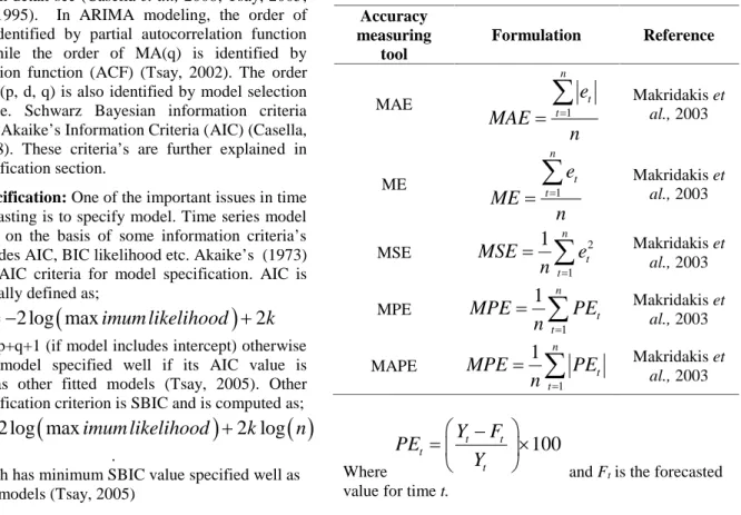
Forecasting Accuracy Measuring Techniques: After model selection, a next important step is to measure the accuracy to verify the reliability of forecasted value based selected model. Various tools are available in literature which includes Root mean square error (RMSE), mean absolute error (MAE), mean absolute percentage error (MAPE), mean error (ME) and mean percentage error (MPE). Further computation and literature of these accuracy measuring tools are given in table 2;
Table 2. Forecasts accuracy measuring tools Accuracy measuring tool Formulation Reference MAE 1 n t t
e
MAE
n
Makridakis et al., 2003 ME 1 n t te
ME
n
Makridakis et al., 2003 MSE 2 11
n t tMSE
e
n
Makridakis et al., 2003 MPE 11
n t tMPE
PE
n
Makridakis et al., 2003 MAPE 11
n t tMPE
PE
n
Makridakis et al., 2003 Where100
t t t tY
F
PE
Y
and Ftis the forecasted value for time t.RESULTS AND DISCUSSION
In this research, time series models were fitted on wheat production data of Pakistan. The objective of fitting multiple time series models on this data is to obtained reliable forecasts on the basis of statistical measures.
Wheat production Forecasting 1902-2005
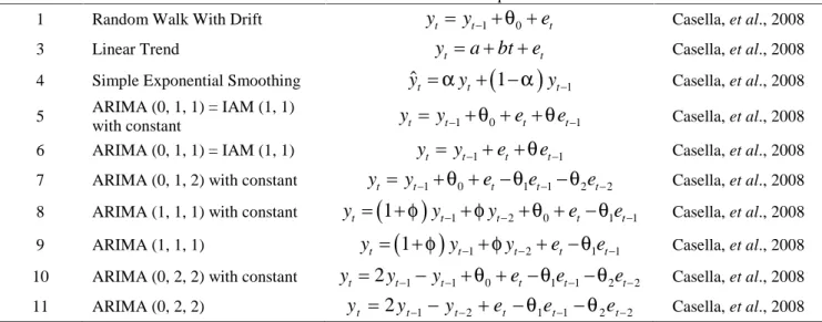
In table 4, different time series models fitted and results are presented with model selection and validity criteria’s. On the basis of AIC we have found that Model M i.e. ARIMA(1, 2, 2) has lowest AIC and we use this model to forecast wheat production of Pakistan on the basis of historical data i.e. 1902-2005. In this table we also summarize the results of five tests run on the residuals to determine whether each model is adequate for the data. Note that the currently selected model, model M, passes 4 tests. Since no tests are statistically significant at the 95% or higher confidence level, the current model is probably adequate for the data. Similar results are also obtained by using JMP Software as on the basis of AIC and SBC ranks the best selected model is ARIMA (1, 2, 2) and the results are shown in table 3. The ARIMA(1,2,2) model coefficient summary is given in table 5.
Table 3. Model Comparison Using JMP8 of Wheat Production Forecasting 1902-2005 of Pakistan
Model Comparison Using Statgraphics 15
Models
(A) Random walk with drift = 196.165 (B) Constant mean = 6761.69
(C) Linear trend = -305605. + 159.901 t (H) Simple exponential smoothing with alpha = 0.7077
(I) Brown's linear exp. smoothing with alpha = 0.197 (J) Holt's linear exp. smoothing with alpha = 0.1112 and beta = 0.6644 (M) ARIMA(1,2,2) (N) ARIMA(0,2,2)
(O) ARIMA(1,1,2) (P) ARIMA(0,2,2) with constant (Q) ARIMA(1,0,1) with constant
Table 4. Model Selection and validity model testing criteria’s of Wheat production Forecasting based on 1902-2005
Model eRMSE MAE MAPE ME MPE AIC RMSE RUNS RUNM AUTO MEAN VAR
(A) 851.908 618.639 13.0096 8.83005E-14 -3.73582 13.5142 851.908 OK OK OK OK ** (B) 5577.81 4637.86 97.1633 -3.53304E-12 -67.0982 17.2723 5577.81 * *** *** *** *** (C) 2814.55 2365.87 53.832 -2.96635E-11 -5.30844 15.9236 2814.55 * *** *** OK ** (H) 833.578 605.206 11.8379 262.469 1.70305 13.4707 833.578 OK OK OK ** *** (I) 733.613 541.758 11.1163 118.53 0.52926 13.2152 733.613 * OK OK OK ** (J) 717.878 543.487 11.6289 31.8212 -1.23138 13.1911 717.878 OK OK OK OK *** (M) 705.377 538.004 10.7913 43.3898 -0.236575 13.1752 705.377 OK OK OK OK *** (N) 721.774 538.285 10.8728 53.2794 -0.481246 13.2019 721.774 OK OK OK OK *** (O) 728.637 535.153 10.8385 75.1509 -0.0492618 13.24 728.637 OK OK OK OK *** (P) 735.449 540.974 11.0765 -2.79145 -2.77791 13.2587 735.449 OK OK OK OK ** (Q) 740.586 538.79 10.9465 41.5256 -1.43001 13.2726 740.586 OK OK OK OK ** Table 5. ARIMA (1,2,2) Model Coefficient Summary
Parameter Estimate Stnd. Error t P-value
AR(1) 0.209104 0.0995956 2.09954 0.038313
MA(1) 1.85085 0.0314206 58.9058 0.000000
MA(2) -0.928474 0.0350945 -26.4564 0.000000
On the basis of Table 5, model coefficients the estimated wheat forecasted model is;
2 1 1
1
.
85085
ˆ
0
.
928472
ˆ
ˆ
209104
.
0
ˆ
t
y
t
e
t
e
ty
Where
y
ˆ
tis the forecasted wheat production for time t years.1
ˆ
ty
is the forecasted wheat production of one previous year
1
ˆ
te
is the previous one year residual as indicated in appendix
2
ˆ
te
is the previous two year residual as indicated in appendix table
Testing Selected Model Assumptions (Normality, Autocorrelation and Heteroscedasticity): We get the reliable wheat production future value if the selected
the assumptions i.e. Normality, Autocorrelation and Heteroscedasticity of the selected model residuals. Table 6. Tests for Autocorrelation and Independence
Test Test Statistic
Value
p-value Runs above and below
median
0.4975 0.6188
Runs up and down -0.0394 1.0000
Box-Pierce Test 15.3043 0.8074
Table 6, indicated that the ARIMA (1, 2, 2) model residuals are uncorrelated as well as independent as all three tests signify.
Three tests have been run to determine whether or not the residuals form a random sequence of numbers. A sequence of random numbers is often called white noise, since it contains equal contributions at many frequencies. The first test counts the number of times the sequence was above or below the median. The number of such runs equals 49, as compared to an expected value
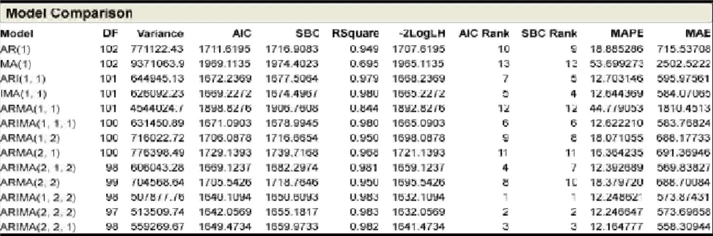
of 52 if the sequence were random. Since the P-value for this test is greater than or equal to 0.05, we cannot reject the hypothesis that the residuals are random at the 95.0% or higher confidence level. The second test counts the number of times the sequence rose or fell. The number of such runs equals 68, as compared to an expected value of 67.67 if the sequence were random. Since the P-value for this test is greater than or equal to 0.05, we cannot reject the hypothesis that the series is random at the 95.0% or higher confidence level. The third test is based on the sum of squares of the first 24 autocorrelation coefficients. Since the P-value for this test is greater than or equal to 0.05, we cannot reject the hypothesis that the series is random at the 95.0% or higher confidence level. The normality is also tested by normal probability plot as shown in figure (1) and periodogram as shown in figure (4) both figures indicated that the residuals of ARIMA (1, 2, 2) are normally distributed. The heteroscedasticity is tested by Var test as show in Table 3 indicated that ARIMA (1, 2, 2) residuals are heteroscedastic. There is no indication of autocoorelation in residuals of selected model signifies by runs and Box-Pierce test.
Residual Normal Probability Plot ARIMA(1,2,2) 0.1 1 5 20 50 80 95 99 99.9 percentage -1700 -700 300 1300 2300 3300 R es idual
Figure 1. Residuals Normal Probability Plot of Wheat Production Model for 1902-2005
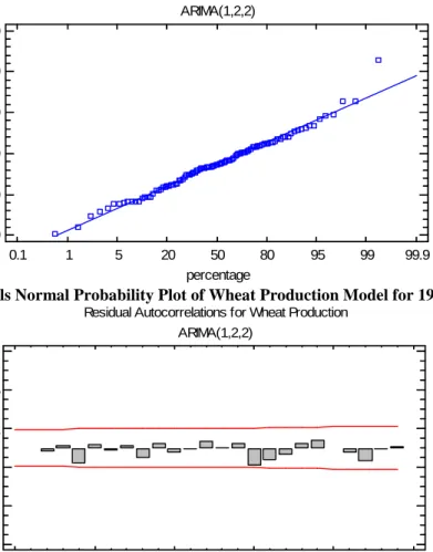
Residual Autocorrelations for Wheat Production ARIMA(1,2,2) 0 5 10 15 20 25 lag -1 -0.6 -0.2 0.2 0.6 1 A ut oc or rel at ions
Residual Partial Autocorrelations for Wheat Production ARIMA(1,2,2) 0 5 10 15 20 25 lag -1 -0.6 -0.2 0.2 0.6 1 P ar ti al A ut oc or rel at ions
Figure 3. Residuals Partial Autocorrelation Plot of Wheat Production of ARIMA (1, 2, 2)
Periodogram for Residuals
0 0.1 0.2 0.3 0.4 0.5 0.6 frequency 0 0.2 0.4 0.6 0.8 1 O rd in a te
Figure 4. Periodogram of Residuals for Wheat Production ARIMA (1, 2, 2) Model Table 7. One step ahead forecasts and residuals for wheat production data (1902-2005)
year Data Forecast Residual
2006 21277 21440.7 -164
2007 23295 21705.9 1589
2008 20959 22062.4 -1104
2009 24033 22438 1595
2010 23311 22817.6 493
Table 8. Wheat production forecasts (in thousand tons) with interval of 10 years
Year 2020 2030 2040 2050 2060
Forecast 26623.5 30429.8 34236 38042.2 41848.5
One step ahead forecasts and residual of wheat production on the basis of 1902 to 2005 wheat production data for the year 2006 to 2010 is presented in table 7. Wheat production forecasted value on the basis of ARIMA (1,2,2) model with interval of 10 year from 2020 to 2060 is presented in table 8 . From table 6, we have found that wheat production of Pakistan would become
26623.5 thousand tons in 2020, 30429.8 in 2030, 34236 in 2040, 38042.2 in 2050 and 41848.5 thousand tons in 2060. As the forecasting is based on sound statistical formulation, so it is adequate forecasting provided that the environmental conditions remain same.
Conclusion: As the population increases over time gradually, therefore it is necessary to plan to meet the requirements of nation. For this purpose, forecasting is the key tool to alarm about the need of nation in advance. Wheat is the basic need of any country all over the world. In this study, we developed time series models to forecasts wheat production of Pakistan on the basis of historical data i.e. 1902-2005. We have developed different time series models on wheat production of Pakistan on this data. Best model is selected on the basis of model selection criteria i.e. AIC and SBIC. Main interest of developing time series model as other studies is that the model fitted is also satisfied residual assumptions i.e. normality, independence and no autocorrelation. On the basis of these model selection criteria, we have found that best model for wheat production forecasting of Pakistan is ARIMA (1, 2, 2). On the basis of developed time series model, we have found that best time series model for forecasting wheat production of Pakistan is ARIMA (1, 2, 2) because this model has lower AIC and SBIC as compared to other fitted time series models. On the basis of this model, we have found that wheat production of Pakistan would become 26623.5 thousand tons in 2020 and would become double in 2060 as compared in 2010 under the assumption that there is no irregular movement or variation is occurred.
REFERENCES
Boken, V.K. (2000). Forecasting spring wheat yield using time series analysis: a case study for the Canadian Prairies. Agron. J, 92:1047-1053. Box, G.E.P. and G.M. Jenkin (1970). Time Series
Analysis, Forecasting and Control. (San Francisco: Holden-Day,).
Box, G.E.P. and D.A. Pierce (1970). Distribution of residual autocorrelations in autoregressive-integrated moving average time-series models. J. Amer. Stat. Asso. 65:1509-26.
Box, G.E.P., G.M. Jenkins and G.C. Reinsel (1994). Time series Analysis, Forecasting and Control. 3rd Ed. Englewood Cliffs, N J: Prentice-Hall. Chatfield, C. (1995). The Analysis of Time Series an
Introduction. 5thEd. Chapman & Halljcrc Boca
Raton London New York Washington, D.C. Elivli, S., N. Uzgoren and M. Savas (2009). Control
charts for autocorrelated colemanite data. J.Sci. Indust Res. 68: 11-17.
Government of Pakistan. (2004). Economic Survey 2003–2004 Finance Division. Economic Adviser’s Wing, Islamabad.
Hamid, N.P., V. Thomas, Alberto and G. Suzanne (1987). The wheat economy of Pakistan setting and prospects. International Food Policy Research Institute, Ministry of Food and Agriculture, Government of Pakistan, Islamabad, Pakistan. Iqbal, N., K. Bakhsh, K. Maqbool, and A.S. Ahmad
(2000). Use of the ARIMA model for forecasting wheat area and production in Pakistan. Int. J. Agri. Biol. 2: 352-354.
Karim, R., A. Awal and M. Akhter (2005). Forecasting of wheat production in Bangladesh. J.Agri. Soc. Sci. 1: 120–122.
Makridakis, S., S.C. Wheelwright and R.J. Hyndman (2003). Forecasting: methods and applications. 3rdEd. John Wiley and Sons.
Muhammad, K. (1989). Description of the historical background of wheat improvement in baluchistan, Pakistan. Agriculture Research Institute (Sariab, Quetta, Baluchistan, Pakistan). Muhammad, F., M. Siddique, M. Bashir and S. Ahmad
(1992). Forecasting rice production in Pakistan using ARIMA Models. J.Anim.Plant.Sci. 2: 27– 31.
Sabir, H.M. and S.H. Tahir, (2012). Supply and demand projection of wheat in Punjab for the year 2011-2012. Interdis. J. Contemp. Res. Bus. 3: 800-808.
Saeed, N., A. Saeed, M. Zakria and T.M. Bajwa (2003). Forecasting of wheat production in Pakistan using arima models. Int. J. Agri. Biol. 2:352-353.
Tsay, R.S. (2002). Analysis of Financial Time Series: Financial Econometrics. John Wiley & Sons, Inc.
Qureshi, K., A.B. Akhtar, M. Aslam, A. Ullah andA. Hussain (1992). An Analysis of the relative contribution of area and yield to Total production of wheat and maize in Pakistan. J. Agri. Sci. 29: 166–169.
Shabur, S.A. and M.E. Haque (1993). An analysis of rice price in Mymensing town market pattern and forecasting. Bang. J. Agri. Econo. 16: 61-75. Sohail, A., A. Sarwar and M. Kamran (1994). Forecasting
total food grains in Pakistan. J. Engi. Appl. Sci. 13: 140- 146.
Appendix ARIMA (1, 2, 2) 1902-2005 Period(t) Wheat Production
y
t Forecasted value of wheat production
y
ˆ
t Residual
e
ˆ
t 1902 1407 1903 1931 1904 2795 2244.67 550.329 1905 2491 2464.92 26.0801 1906 3972 2405.46 1566.54 1907 2520 2951.03 -431.034 1908 2099 2706.97 -607.967 1909 2770 2618.64 151.36 1910 2916 2824.72 91.2836 1911 2913 2923.8 -10.8009 1912 2801 2983.59 -182.589 1913 2475 2994.12 -519.124 1914 2670 2895.55 -225.545 1915 3230 2909.4 320.599 1916 2185 3063.53 -878.53 1917 2557 2728.08 -171.084 1918 3174 2726.26 447.74 1919 2372 2854.68 -482.683 1920 3034 2582.37 451.629 1921 1793 2718.07 -925.072 1922 3251 2285.57 965.429 1923 2887 2627.6 259.398 1924 2864 2558.28 305.721 1925 2248 2587.3 -339.304 1926 2545 2419.86 125.143 1927 2598 2486.26 111.744 1928 1737 2509.35 -772.349 1929 2781 2218.13 562.865 1930 3329 2464.46 864.543 1931 2731 2695.75 35.2521 1932 2599 2630.83 -31.8252 1933 2639 2656.08 -17.077 1934 2782 2717.02 64.9758 1935 2866 2810.42 55.5784 1936 2962 2895.12 66.8763 1937 3184 2988.33 195.666 1938 3080 3132.29 -52.2913 1939 3146 3186.29 -40.2861 1940 3594 3273.56 320.44 1941 3137 3491.39 -354.387 1942 3743 3444.2 298.802 1943 4168 3689.2 478.8 1944 3495 3946.39 -451.394 1945 3824 3872.42 -48.4207 1946 3506 4033.03 -527.035 1947 3115 3983.22 -868.215 1948 3354 3826.34 -472.337 1949 4038 3792.85 245.154 1950 3924 3922.76 1.24372 1951 3993 3868.45 124.549 1952 3010 3870.9 -860.899 1953 2405 3516.06 -1111.06 1954 3645 3136.13 508.872 1955 3186 3297.36 -111.361 1957 3639 2993.37 645.625 1958 3564 3027.63 536.367 1959 3907 3023.78 883.223 1960 3909 3200.69 708.308 1961 3814 3348.77 465.228 1962 4027 3495.29 531.707 1963 4170 3752.24 417.756 1964 4162 4018.83 143.165 1965 4591 4245.32 345.678 1966 3916 4604.51 -688.505 1967 4335 4605.42 -270.423 1968 6419 4844.02 1574.98 1969 6618 5685.01 932.987 1970 7295 6158.35 1136.65 1971 6476 6834.43 -358.43 1972 6890 7062.93 -172.933 1973 7442 7549.11 -107.106 1974 7629 8060.53 -431.53 1975 7674 8438.93 -764.93 1976 8621 8704.42 -83.4166 1977 9144 9200.79 -56.7865 1978 8367 9605.99 -1238.99 1979 9950 9558.63 391.367 1980 10857 10151.8 705.248 1981 11475 10680.7 794.291 1982 11915 11217.3 697.743 1983 12414 11763.8 650.162 1984 10882 12369.8 -1487.82 1985 11703 12282.7 -579.701 1986 13923 12707.6 1215.44 1987 12882 13647.7 -765.706 1988 12675 13704.8 -1029.82 1989 14419 13837.5 581.499 1990 14316 14538.5 -222.533 1991 14565 14778.6 -213.566 1992 15684 15076.3 607.732 1993 16157 15661.8 495.192 1994 15213 16142.7 -929.655 1995 17002 16153.1 848.875 1996 16907 16928.2 -21.1805 1997 16651 17245.4 -594.407 1998 18694 17441.8 1252.17 1999 17858 18348.3 -490.255 2000 21079 18490 2589.01 2001 19024 19901.3 -877.264 2002 18226 19893.3 -1667.28 2003 19183 19962.2 -779.223 2004 19500 20401.2 -901.177 2005 21612 20627.6 984.369