DOI: 10.12928/TELKOMNIKA.v15i3.4028 1290
Regression Modelling for Precipitation Prediction Using
Genetic Algorithms
Asyrofa Rahmi, Wayan Firdaus MahmudyFaculty of Computer Science, Universitas Brawijaya, Malang, Indonesia Corresponding author, e-mail: [email protected], [email protected]
Abstract
This paper discusses the formation of an appropriate regression model in precipitation prediction. Precipitation prediction has a major influence to multiply the agricultural production of potatoes in Tengger, East Java, Indonesia. Periodically, the precipitation has non-linear patterns. By using a non-linear approach, the prediction of precipitation produces more accurate results. Genetic algorithm (GA) functioning chooses precipitation period which forms the best model. To prevent early convergence, testing the best combination value of crossover rate and mutation rate is done. To test the accuracy of the predicted results are used Root Mean Square Error (RMSE) as a benchmark. Based on the RMSE value of each method on every location, prediction using GA-Non-Linear Regression is better than Fuzzy Tsukamoto for each location. Compared to Generalized Space-Time Autoregressive-Seemingly Unrelated Regression (GSTAR-SUR), precipitation prediction using GA is better. This has been proved that for 3 locations GA is superior and on 1 location, GA has the least value of deviation level.
Keywords: precipitation prediction, regression models, genetic algorithms
Copyright © 2017 Universitas Ahmad Dahlan. All rights reserved.
1. Introduction
As a country rich in fertile agriculture land, one crop that has been grown is the potato. The amount of carbohydrate in potatoes became one of the objectives to strengthen the stability of food. Therefore, raising the production needs to be considered carefully. It also became the main destination for farmers in Indonesia. In Indonesia, Tengger is a region in East Java that farm lot planted with potatoes. There are four areas in Tengger namely Puspo, Sumber, Tosari and Tutur. Ways to improve potato production is following the pattern of planting in accordance with the natural condition of the area at that time. To determine the appropriate planting pattern, it can be seen from its historical data or the original weather data on previous days. By observing and implementing the pattern of planting whose natural conditions in accordance with the climatic conditions in the area, the production of potatoes obtained is maximum [1, 2].
Climatic conditions can be identified by predicting precipitation [3]. But this time, the precipitation of an area is difficult to predict because of the impact of global warming. Based on historical data, the precipitation illustrates that the data properties are non-linear [4].
Some techniques have been implemented in precipitation prediction. Using statistical model, precipitation can be predicted. The first model is Generalized Space-Time Autoregressive–Seemingly Unrelated Regression (GSTAR-SUR) in 4 places [1]. This model has been used to predict the precipitation based on the relationship of several locations around. Then precipitation has been studied using Autoregressive Moving Average (ARMA/ARIMA) [2, 5]. The linear approach has been tried using Multiple Linear Regression [6] and many methods have been applied using non-linear approach. Completion using Markov [7] and Decision Tree [8] have been performed in precipitation prediction. Besides, Fuzzy Logic [9, 10] also have been tried also Genetic Programming [11], SVM, and SVR [4, 12]. Combining of 2 methods have been studied using Fuzzy-Markov [13] and Fuzzy-GA [14]. The techniques implemented before is capable enough to predict the precipitation but the level accuracy obtained is still far from expectations. Then the other techniques are good enough but to get the formulation are still requires a lot of trials so ineffective.
Based on the similarity data of this study, precipitation prediction has been tried to solve using GSTAR-SUR [1] and Fuzzy Logic [10]. This study aims to improve the previous methods. To solve the problems in predicting precipitation, the approach used is non-linear regression
and genetic algorithms is used to select the best independent variables. Such as previous methods, for some problems, GAs can be implemented using regression and has been shown to provide more optimal results even using linear regression [15, 16]. Besides, according to study that has been conducted by Majda and Harlim, one of the non-linear regression approach that has proven the optimization than the other is a quadratic regression model [17].
In predicting precipitation optimal using quadratic regression, there is some precipitation that period is not too have a strong influence in the movement pattern of precipitation. Therefore, it needs to be selected in the period of the precipitation. However, to look for the corresponding period, the problem is to have a lot of combinations of the period that may be an optimal solution in predicting precipitation. If using the 20 periods the previous precipitation then it is likely to look for a solution that is as many as 220 is 1048576 combinations. The number of combinations of solutions that need to be searched also requires a lot of time. So, in order to save time in the process of finding an optimal solution is to use a genetic algorithm.
This paper details an extension study of Rahmi, Mahmudy, and Setiawan [18]. The previous study has applied GAs to find the most optimal number coefficients to form a regression model that produces the minimal error. In that study, the coefficient of the regression model is the entire period without considering which periods that most influential or not. This study focuses on the formation of a regression model to choose how many periods are most influential in predicting precipitation and also involves non-linear factors. Then the result of the study provides better accuracy in predicting precipitation than the previous study [1, 10].
2. Regression Models
The prediction results in the regression model represented by the symbol Y as the dependent variable that is influenced by several variables that indicate the data [X1, X2, … , Xk].
Regression equation used to examine the relationship dependent variable and several independent variables [15, 16]. The composition of multiple regression models in general [16] is shown in Equation (1).
(1)
Where k specifies the number of data in the past, b1, b2, …, bk are regression
coefficient, and is an independent variable in the form of random errors which has a mean of zero and a variance in influencing the value of so that the Equation (1) can be transformed into Equation (2).
(2)
Where t is time. So Equation (2) read that to find predictions on this period (t), then require data on the previous period (t-1), data on 2 periods before (t-2) and data on k periods before (t-k).
Equation (1) and (2) are multiple linear regression. For predicting, a non-linear regression model can also be done. Determining the patterns of regression in predicting, it can use another model of regression such as quadratic regression model. This model requires that the elasticity of substitution becomes greater than zero and also diminishing marginal returns must be valid so that appropriate to the effects of the problem. Quadratic regression is shown in Equation (3) [17].
(3)
The quadratic regression is figured in Equation (3). Generally, quadratic regression has an intercept, coefficients that apply using the single variable (X), and square variable (X2). According to Equation (1), (2) and (3), non-linear prediction used is shown in Equation (4).
Multiple non-linear regression models is shown in Equation (4). This equation consists of intercept, multiple coefficients using variable and the square variable.
3. Methodology
Precipitation data used in this study is from 2005 through 2013 obtained since the start of the dry season as training data. Each one data represents the period of 10 days which has a value less than or equal to 50 mm. Then, the following data is representative of the next 10 days which also has a value less than or equal to 50 mm.
There are 4 locations that have identified to be studied, Puspo, Sumber, Tosari and Tutur. Overall precipitation data is divided into two types. Training data to determine the best regression model based on the historical data and testing data to see the results of prediction. The amount of data used is 320 for training and 100 for testing. Table 1 shows the precipitation data of Puspo area.
Table 1. Precipitation Data of Puspo Area [1]
No YT Xt-1 Xt-2 … Xt-29 Xt-30 Xt-1 2 Xt-2 2 … Xt-29 2 Xt-30 2 1 4.5 14.5 5.364 0 0 14.52 5.3642 02 02 2 14.5 5.364 7.4 0 4.8 5.3642 7.42 02 4.82 3 5.364 7.4 25.8 4.8 0 7.42 25.82 4.82 02 … 320 18.7 19.5 12.5 0 0 19.52 12.52 02 02
Each row of Table 1 shows the original precipitation symbolized by Yt, then followed by
30 periods of precipitation symbolized by X, where Xt-1 is the precipitation of a period ago, then
Xt-2 is the precipitation of two periods before prior to the Xt-30 is precipitation 30 periods in
advance. Then because of the non-linear regression model used is quadratic then 30 of the next field contains 30 squares of the same period the precipitation as before.
Precipitation prediction system implements regression model and genetic algorithm (GAs). GAs applied to form new model and select the best equation of regression model. The best equation regression resulted is shown which periods have increasingly influenced to predict the precipitation on the next days. The regression model resulted is applied to compute the prediction and error that used as a benchmark the best regression model.
GAs concept imitates natural and biological selection process [19-21]. Only the best individuals indicated by fitness in order to survive in the next generation (iteration), then they would be an optimal solution of a problem. The advantages of stochastic nature of Genetic Algorithm are able to find the solution to the problems that are diverse and large-scale. Process in the genetic algorithm starts with initialization phase, which creates individuals or chromosomes that have a string of arrays which randomly generated. Each chromosome represents a possible solution to a problem. By considering the fitness of a chromosome, the greater fitness indicates that the chromosome is more qualified to be a solution [22]. The final stage is the selection of choosing the new individuals as many as the population size obtained by the individual parents and offsprings. The individuals results of the selection process are alive in the next generation as the new population.
3.1. GAs Cycle
There are 2 kinds of cycles GAs. The selection process is used to select parent (individual) in the first type of GAs [19, 22]. However, in this study using the other cycle one. It is the parent chosen randomly and after the reproduction process is completed, the next stage is to the selection process [20]. The overall GAs Cycle is shown as following:
Step 0 : Determining GAs parameters
Parameters on GAs are population size (popSize), crossover rate (Cr), mutation rate (Mr) and maximum generation (maxGen)
Step 1 : Initialization of population
Let generation gen = 0, Generate the chromosome randomly as many as popSize Step 2 : Reproduction
Through crossover operator to produce offspring using popSize x Cr and mutation operator to produce offspring using popSize x Mr
Step 3 : Selection
Select the popSize of chromosome from the collection of parents population and offsprings
Step 4 : Let gen = gen + 1
When gen is equal to maxGen then stop, else do step 2. 3.2. Chromosome Representation
The candidates of optimal solution set at the time of chromosomes representation. The visual representation of chromosomes that are used to solve problems in this study is shown in Figure 1.
Figure 1. A Chromosome Representation
Chromosome representation shown in Figure 1 defines a chromosome that consists of two segments with a length of 61 genes. The first gen is intended for choice using intercept or not, the first 30 genes is single data for 30 periods before (t-30) at the location and the second 30 genes are intended for the squared data of 30 periods before (t-30).
The binary representation is a type of chromosome formation used in this study so the content of each gene on the chromosome is 0 or 1. 0 represents the period data that has been excluded and 1 represents the period data that has been included. The function of the binary representation itself is to determine data on which periods that have been related to the prediction. Then, the 1st gene of a chromosome is 1 which means the intercept is used. The 2nd gene is 1, which means the precipitation on a period before (Xt-1) is used and the 3
rd
gene worth 0 which means that the precipitation on two days earlier (Xt-2) is not be used, and so on until the
square precipitation value. The population is obtained from the set of chromosomes that have represented a number of population size (popSize) which has been initialized in the beginning. So, if the value of popSize is 10, then the population consists 10 chromosomes.
3.3. Fitness Function
The next process is to calculate the fitness of a chromosome (individual) that has been presented. The chronology of fitness calculation is using the chromosome to change the precipitation data based on the gene value. According to the new precipitation data that has been changed, the data is processed using regression analysis then the coefficient regression has been formed. From regression coefficient and the new precipitation data then the predicted results can be generated. Forms regression model is considered good if obtaining prediction results closer to the original results. One of the ways is using Root Mean Square Error (RMSE). The smaller value of RMSE indicates a predicted value is closer to its original value. Thus, in GAs process, the regression coefficients model formed from chromosome is said to be optimal to be a solution if they have a great fitness value, while the proximity of good value is to have a small RMSE, then the fitness value is inversely proportional to the value of RMSE. Equation (5) is RMSE function and to get the fitness value using Equation (6)
√∑ (5)
Where n is the number of data used to predict. For training process, the amount of data predicted as many as 320, so that the value of n is 320 so do the testing process, n is 100.
Examples fitness calculation process on one chromosome is shown in Figure 1 as the formation of a model in Table 1. After the precipitation data in Table 1 was processed based on the chromosome on Figure 1, Table 2 is formed as new precipitation data of Puspo Area.
Table 2. New Precipitation Data of Puspo Area Referring to Figure 1
No YT Xt-1 Xt-2 … Xt-29 Xt-30 Xt-12 Xt-22 … Xt-292 Xt-302 1 4.5 14.5 0 0 0 14.52 5.3642 0 02 2 14.5 5.364 0 0 0 5.3642 7.42 0 4.82 3 5.364 7.4 0 4.8 0 7.42 25.82 0 02 … 320 18.7 19.5 0 0 0 19.52 12.52 0 02
New data generated in Table 2 very different with Table 1. In Table 2, The Yt columns to
be equal to Yt column in Table 1 because it serves as an original value of precipitation. The next
column in Table 2 is Xt-1 also has the same value as the column Xt-1 in Table 1 because the
value of chromosomes in Figure 1 with a column Xt-1 is 1 which means that the variable Xt-1 is
used. Unlike the Xt-2 column in Table 2 are worth 0. This value differs from Xt-2 column in Table
1 which is 5.364. This change occurred because the column Xt-2 in Figure 1 has a value of 0
which means that the variable Xt-2 is not used.
The next process is calculating regression coefficients based on Table 2 through a process of regression analysis. After the coefficient of each variable is obtained, then the regression model are formed.
The regression coefficients model that have been obtained, is used to predict overall precipitation based on the data in Table 2. Next, proceed by searching for RMSE values based on Equation 5 to obtain fitness values using Equation 6.
3.4. Initialization Population
The population is the number of representation chromosome of the population size that has been initialized at the beginning of the process in initialization parameters. A population reflects the pool of possible solutions to a problem [21]. The example population and its fitness of popSize 10 are shown in Table 3.
Table 3. An Initialization Population
P I Xt-1 Xt-2 … Xt-30 Xt-1 2 Xt-2 2 … Xt-29 2 Xt-30 2 Fitness 1 1 1 0 0 1 1 0 1 0.1703 2 1 0 0 1 1 0 1 1 0.1655 3 0 1 1 0 1 1 1 0 0.1673 … 10 0 1 0 0 0 0 1 1 0.1529 3.5. Reproduction
Reproduction is the operator of the formation of offspring (children / new individual) from the individual parent population. The purpose of reproduction is to get the new individual who has the diversity is not too far away from its parent so that it can obtain a more diverse solution to resolve the problems [23]. Operator reproduction consists of two processes, namely crossover and mutation [20].
3.5.1. Crossover
The number of offspring result of the crossover derived from multiplying the value of Cr and the size of the population (10) that has been initialized at the beginning (popSize). If Cr value is 0.5 then the offspring resulted from crossover process is (10x0.5) 5. 5 offsprings (C1-C5)
produced from the crossover process included in the offspring pool for each generation.
In this study, the type of crossover used is the one-cut-point crossover. At this crossover types, starting with determining the second parent (parent individuals) and the cutoff point (gen). Then performed a cross between parents beginning of the first gene to gene corresponding point of the intersection with the second parent of the gene point of the intersection until the last gen. Examples crossover process determines the two parents (Parent 1 and Parent 2) and a randomly cut point on the 31st gen.
Figure 2. One-Cut Point Crossover Process
3.5.2. Mutation
Multiplying the value of Mr and size of the population that has been initialized at the beginning is used to determine the number of offspring of the mutation process. If Mr value is 0.5 then the offspring resulted from mutation process is (10x0.5) 5. 5 offsprings (C6-C10)
produced from the mutation process also included in the offspring pool for each generation. In this study, the mutation process chooses one parent and one gene randomly. Then the value of the altered gene, if the value is 0 then it converted into 1 and vice versa.
Figure 3. Binary Mutation Process
3.6. Selection
The next stage is a selection process which aims to select the best individuals as many as the population size of individuals parent in pool population (P) before and the new individuals (offspring/C) of the reproduction process. Selection type used in this study is the selection of the replacement. This selection model is quite effective in some cases optimization [21]. The virtue of this kind of selection is allowing some individuals with low fitness value to be chosen as the solution to the next generation or iteration because individuals with low fitness are also likely to produce new and better individuals. Table 4 is the selection process using replacement. This process starts from the fitness of overall results of reproduction process (offspring). C1 to C5 are
from crossover process and the other from mutation process.
On Table 4 there are 5 main columns. The first column is offspring symbolized by C and the fitness of offspring on the second column. The third column is the original parent (OP) of offspring. This column describes the origin parents of offspring. OP column has four sub-columns. Original Parent 1 (OP1), Original Parent 2 (OP2), the fitness value of OP1 and Fitness
value of OP2. For offsprings from crossover process have two parents, OP1 and OP2 while the
mutation process have only one parent, OP1. Referring to offspring pool, offsprings from number
1 to 5 are from crossover process and the other are mutation process. The fourth main column is a weak parent (WP). WP column has two sub-columns, WP itself and its fitness value. WP column is a column contains a parent of original parents (OP), who has the weakest fitness. If offsprings are from crossover process that has two original parents, the fitness of both original
parents are compared. The original parent with the weakest fitness value is included in WP column. The last main column is Result (R) Column. R column has three sub-columns. Chosen Individual column and its fitness value also the description of it. Chosen individual is a column containing the results of the comparison offspring itself with its parent regarding the fitness value. The great value is the winner to be the chosen individual. If the offspring is the winner then the description is “changed”. The meaning is the offspring replaced the weakest parent position on population.
Table 4. Replacement Selection Process C Fitness
Original Parent (OP) Weak Parent (WP) Result (R) OP1 OP2 Fitness OP1 Fitness OP2 WP Fitness WP Chosen
Individual Fitness Description
1 0.1682 P1 P2 0.1703 0.1655 P2 0.1655 C1 0.1682 Changed 2 0.1463 P1 P20 0.1703 0.1529 P20 0.1529 P20 0.1529 Fixed … 6 0.1627 P3 0.1673 P3 0.1673 P3 0.1673 Fixed … 10 0.1722 P1(C1) 0.1682 P1 0.1682 C10 0.1722 Changed
For the selection process, there are 4 conditions that need to be considered. For first offspring (C1), the fitness value is 0.1682. The original parents (OP) of C1 are two, there are OP1
and OP2. OP1 is P1, where P is Parent and OP2 is P2. Then find WP based on the fitness value
of OP1 and OP2. P2 is the weak parent because the fitness is 0.1655. After that, the fitness of
WP compared to the fitness of C1. The fitness of C1, 0.1682, is greater than WP, 0.1655. So C1
changed/replaced WP on population. The second condition is applied if the fitness of WP greater than the offspring such as C2 case. Then the WP (P20) is fixed.
Next condition is for offspring of mutation process. The third condition is C6. Because
the original parent of mutation process is only one (P3), so that parent has been WP directly and
the fitness compared to the fitness of C6. Because fitness of P3 is greater than WP then P3 is
fixed. And the last condition is C10 case. OP of C10 is P1. Same as before, the parent has been
WP directly then compared to C10. Because P1 has been changed by C1, so C10 compared to
C1. The fitness of C10 is greater than C1 then C1 or P1 was changed/replaced to C10.
4. Results and Discussion 4.1. Population Size Testing
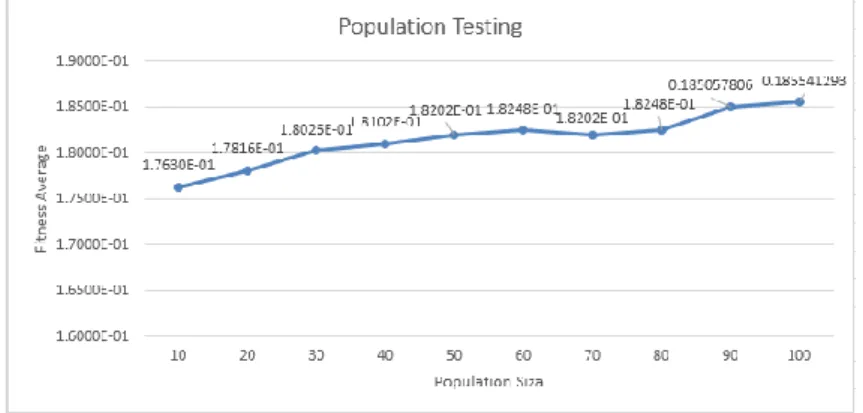
Tested population size is a multiple of 10. The initial value generation number is 100 with combined value of Cr and Mr are 0.5 and 0.5. Tests performed 10 times and recorded their average fitness which is calculated to determine the optimum population size. The purpose of the calculation of average fitness is to represent the optimal solution due to the stochastic nature of the genetic algorithm so that always gives results that can vary each executed. Figure 4 is a graph of the results of population testing to choose the optimal population size.
Based on the chart of population testing seen in Figure 4, the range between 10 to 100, the starting point of optimal population size based on the value of fitness is 50. It can be seen in the graph, that the fitness value on the size of the population under 50 has much difference is 0.0059, 0.0019, 0.0021, 0.00076 and 0.000999. Unlike when the points 50, 60, 70 and 80 which have a difference in value that is not too far away. From point 50 to 60, the difference is 0.000467, while at the point of 60 to 70 is 0.0004669 and 0.000465 at point 70 to 80. Within the range of 10 to 100, some of this difference indicates that the start point 50 have said nearly optimal. The starting point from 80 to 100, the resulting fitness value is higher. It is also reasonable. Because it is the first testing so the parameter values of generation, Cr and Mr Combinations used have not been optimized. The next step is necessary to test those parameters in order to get the solutions which achieve optimally.
4.2. Number of Generations Testing
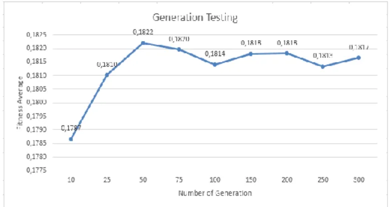
The next parameter testing is a number of generations. The values tested are 10, 25 to 100 which multiples of 25, and 100 to 300 which multiples of 50. The initial value combinations Mr and Cr values are 0.5 and 0.5. However, the population size used is the optimal size on the test results of the previous population testing. Tests performed 10 times and recorded their best fitness value and the average to determine the optimum number of generations. Figure 5 is a trace graph of generation testing.
Figure 5. Generation Testing
According to the graph of generation testing seen in Figure 5, the best average fitness is obtained on the number of generations 50. Since the average yield earned fitness achieve an optimal point in generations to 50. The number of generations that were tested ceases to 300 because after 50 the average fitness obtained have the very little difference and not too far away. The difference only almost 0.0003. If the test that has performed is greater than 300 then the average fitness obtained is not too significant but it requires the longer computing time. 4.3. Testing Combination of Mr and Cr
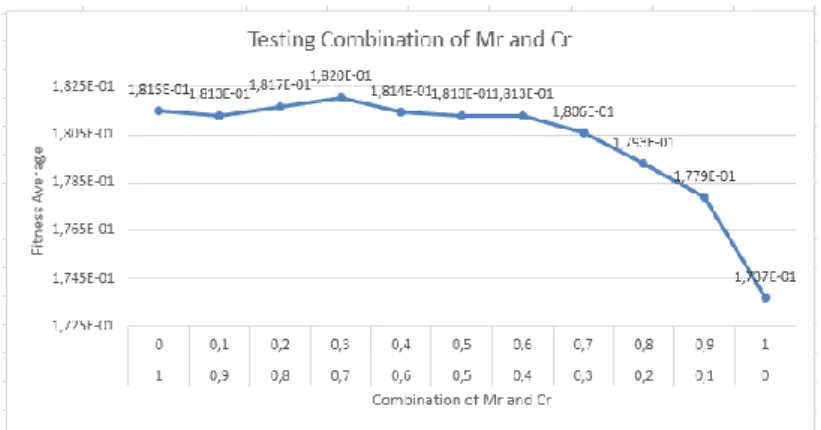
Crossover rate (Cr) and Mutation rate (Mr) are the value that specifies the number of new individuals produced. Cr as a determinant of the number of new individuals of the crossover process and Mr as a determinant of the number of new individuals of the mutation process. Hence, testing the combination of Mr and Cr equal to test the best combination the number of new individual best of exploration and exploitation. The combination of Mr and Cr tested is a value between 0 and 1. For this testing, the size of the population and the number of generations used is the population size and the number of generations previous best in the test population size of 50 and the number of generations 50. Tests performed 10 times and recorded his best fitness value and the average is calculated to determine the optimal combination of Cr and Mr value. Figure 6 is a trace graph testing of combination value of Mr and Cr where the value of Mr starts at 0 and the value of Cr starts at 1.
Figure 6 tests graph of a combination of Mr and Cr. The average fitness of the best combination of value Cr obtained at 0.7 and 0.3 for Mr value. Because the average fitness
results obtained from the combination of the best values of other combinations. When combined value of Cr less it produce an average fitness is not optimal because, in this phase, genetic algorithms which work based on random search is not able to explore the search area effectively.
Figure 6. Testing Combination of Mr and Cr
4.4. Analysis and Testing
Based on the testing parameters that have been done before, it is found that the optimal population size, number of generation, also combination of Cr value and Mr value as shown in Table 5.
Table 5. The Optimal Parameters GAs for Precipitation Prediction
Parameters Value
Population Size 50
Number of Generations 50
Cr Value 0.7
Mr Value 0.3
By using the optimal parameters obtained from testing, the optimal non-linear coefficient is formed based on each location. Optimal coefficients produce a form of regression best to solve the problems precipitation prediction. Based on the non-linear coefficients are formed, the variables that influence and change at every location is different after trying five times. For Puspo area, the influences variables are using intercept, 12 variables of X dan 11 variables of X2. In Sumber area using intercept, 11 variables of X dan 11 for X2. Tosari area also using intercept, 17 variables of X and variable of X2 18. The last area is also kept using intercept, variables X 14 dan 17 for X2. Table 6 is the result of precipitation prediction for four locations using some methods.
Table 6. The Precipitation Prediction Result of 4 Locations and Related Methods Locations Original Precipitation GSTAR-SUR [1] Tsukamoto [10] Fuzzy GAs-Non-Linear Regression
Puspo 4.5 2.91 11.9898 2.47
Sumber 0 2.18 11.4797 1.904
Tosari 4.8 1.34 11.411 7.27
Tutur 12.6 1.996 12.3064 11.36
To determine the accuracy of precipitation prediction of each location, then it is tested using 100 test data for each location. The acquisition of precipitation predicted results using Genetic Algorithm – Non-Linear Regression System compared to the precipitation prediction
using previous methods, they are GSTAR-SUR [1] and Fuzzy Tsukamoto [10]. The RMSE value of each method has shown in Table 7.
Table 7. Comparing RMSE Value of GAs Non-Linear Locations GSTAR-SUR [1] Fuzzy
Tsukamoto [10] GAs-Non-Linear Regression Deviation Level (GSTAR-SUR) Puspo 4.90 8.95 5.095 0.038273 Sumber 6.69 9.64 6.03 0.098655 Tosari 7.92 8.81 7.04 0.111111 Tutur 10.89 8.64 4.77 0.561983
Table 7 shows that the optimal precipitation predictions obtained by using Genetic Algorithms are more accurate than Fuzzy Tsukamoto. Compared to GSTAR-SUR, prediction using GAs also give the optimal results on Sumber, Tosari and Tutur area. Precipitation prediction using GAs is not as well as GSTAR. However, the deviation level of GAs and GSTAR on Puspo area shows the least value. This can prove that the result of precipitation prediction using Genetic Algorithm – Non Linear Regression is better than the others. The deviation level on Table 7 only between GAs Non-Linear Regression and GSTAR-SUR Model. The deviation level between GAs Non-Linear Regression and Fuzzy Tsukamoto are not necessary because the value of GAs Non-Linear Regression is overall superior to Fuzzy Tsukamoto. Based on the result that has been declaring, GA-Non-Linear Regression very recommended for solving the problem of precipitation prediction.
5. Conclusion
Predicting precipitation can be done effectively by generating non-linear regression model using genetic algorithm. Non-linear approach undertaken in this study was using multiple quadratic regression models. In the process of finding solutions precipitation prediction, binary chromosome representation model can be implemented to look for whatever period of interrelated so as to calculate a regression coefficient that can be used to calculate the precipitation forecast based on historical data.
A form of regression coefficients is processed using Genetic Algorithms. The best form of coefficients obtained by using the optimal parameters of genetic algorithms. Based on testing, the optimal parameters obtained is population size of 50, generation number 50, appropriate combinations of Cr and Mr value is 0.7 and 0.3. Using the optimal parameters of GAs, the best non-linear coefficient is formed. The variables that influence for each location are different. For Puspo area is using intercept, 12 variables of X dan 11 of X2. In Sumber also using intercept, 11 variables of X dan 11 for X2. Tosari area also using intercept, 17 variables of X and 18 variable of X2. The last area is kept using intercept, variables 14 X dan 17 for X2.
The best precipitation prediction obtained by using a genetic algorithm with optimal parameters of 4 locations in Tengger compared to precipitation prediction from previous studies [1, 10]. Based on the RMSE value of each method on every location, precipitation using GAs-Non-Linear Regression is better than Fuzzy Tsukamoto for each location. Compared to GSTAR-SUR, precipitation prediction using GAs is better. This has been proved that for 3 locations GAs is superior and on 1 location, GAs has the least value of deviation level. So that GAs is recommended for solving precipitation prediction in different locations.
Our next study will consider building more powerful approach by hybridizing GAs with another heuristic method to get a better model with lower RMSE. This hybrid approach has been proven more effective for complex problems [24].
References
[1] A Iriany, W Firdaus, S Handoyo, GSTAR-SUR Model for Rainfall Forecasting in Tengger Region,
East Java. In The 1st International Conference on Pure and Applied Research. University
Muhammadiyah, Malang. 2015.
[2] A Nugroho, BH Simanjuntak. ARMA (Autoregressive Moving Average) Model for Prediction of Rainfall in Regency of Semarang - Central Java - Republic of Indonesia, International Journal of
Computer Science Issues (IJCSI). 2014; 11(3): 27-32.
[3] K Rymuza, E Radzka, T Lenartowicz. Effect of Weather Conditions on Early Potato Yields in East- Central Poland. Communications in Biometry and Crop Science. 2015; 10(2): 65-72.
[4] G Adhani, A Buono, A Faqih. Support Vector Regression Modelling for Rainfall Prediction in Dry
Season Based on. In The 2013 International Conference on Advanced Computer Science and
Information Systems (ICACSIS) 28-29 September. 2013: 315-320.
[5] W Sampson, N Suleman, AY Gifty. Proposed Seasonal Autoregressive Integrated Moving Average Model for Forecasting Rainfall Pattern in the Navrongo. Journal of Environment and Earth Science. 2013; 3(12): 80-86.
[6] MK, et al. Rainfall Forecasting Using Data Mining Technique. International Journal of Engineering
and Technology. 2010; 2(6): 397-401.
[7] M Cai. Study on Variation in Wet and Low Water of Precipitation Prediction based on Markov with
Weights Theory. In 2010 Sixth International Conference on Natural Computation (ICNC 2010). 2010;
8: 4296-4300.
[8] N Prasad. An Approach to Prediction of Precipitation Using Gini Index in SLIQ Decision Tree. In 2013 4th International Conference on Intelligent Systems, Modelling and Simulation 29-31 January. 2013: 56-60.
[9] A Agboola, A Gabriel, E Aliyu, B Alese. Development of a fuzzy logic based rainfall prediction model. International Journal of Engineering & Technology. 2013; 3(4): 427-435.
[10] I Wahyuni, WF Mahmudy. Rainfall Prediction In Tengger Region - Indonesia Using Tsukamoto Fuzzy Inference System. In The 1st International Conference on Information Technology, Information System and Electrical Engineering. 2016.
[11] E Fallah-Mehdipour, O Bozorg Haddad, MA Mariño. Prediction and simulation of monthly groundwater levels by genetic programming. Journal of Hydro-environment Research. 2013; 7(4): 253-260.
[12] K Lu, L Wang. A Novel Nonlinear Combination Model Based on Support Vector Machine for Rainfall
Prediction. In 2011 Fourth International Joint Conference on Computational Sciences and
Optimization. 2011: 1343-1346.
[13] L Sheng, W Cheng, HUI Xia, X Wu, X Zhang. Prediction of Annual Precipitation Based On Fuzzy And
Grey Markov Process. In The Ninth International Conference on Machine Learning and Cybernetics,
11-14 July. 2010(3): 1136-1140.
[14] F Nhita, Adiwijaya. A Rainfall Forecasting using Fuzzy System Based on Genetic Algorithm. In 2013 International Conference of Information and Communication Technology (ICoICT) A. 2013: 111-115. [15] K Phiwhorm, S Arch-int. LDL-Cholesterol levels Measurement using Hybrid Genetic Algorithm and
Multiple Linear Regression. In 2013 International Conference on Information Science and
Applications (ICISA) 24-26 June. 2013: 1-4.
[16] B Stojanovic, M Milivojevic, M Ivanovic, N Milivojevic, D Divac. Advances in Engineering Software Adaptive system for dam behavior modeling based on linear regression and genetic algorithms.
Advances in Engineering Software. 2013; 65: 182-190.
[17] AJ Majda, J Harlim. Physics constrained nonlinear regression models for time series. Nonlinearity. 2013; 26(1): 201.
[18] A Rahmi, WF Mahmudy, BD Setiawan. Prediksi Harga Saham Berdasarkan Data Historis Menggunakan Model Regresi (Stock Price Prediction Based on Historical Data using Genetic Algorithm). DORO : Repository Jurnal Mahasiswa PTIIK Universitas Brawijaya. 2015; 5(12): 1-9. [19] BW Yohanes, Handoko, HK Wardana. Focused Crawler Optimization Using Genetic Algorithm.
TELKOMNIKA Indonesian Journal of Electrical Engineering. 2011; 9(3): 403-410.
[20] WF Mahmudy, RM Marian, LHS Luong. Real Coded Genetic Algorithms for Solving Flexible Job-Shop Scheduling Problem - Part I: Modelling. Advanced Materials Research. 2013; 701: 359-363. [21] WF Mahmudy, RM Marian, LHS Luong. Real Coded Genetic Algorithms for Solving Flexible
Job-Shop Scheduling Problem - Part II: Optimization. Advanced Materials Research. 2013; 701: 364-369. [22] S Sen, P Roy, A Chakrabarti, S Sengupta. Generator Contribution Based Congestion Management
using Multiobjective Genetic Algorithm. TELKOMNIKA Indonesian Journal of Electrical Engineering. 2011; 9(1): 1-8.
[23] MM Bhaskar, S Maheswarapu. A Hybrid Harmony Search Algorithm Approach for Optimal Power Flow. TELKOMNIKA Indonesian Journal of Electrical Engineering. 2011; 9(2): 211-216.
[24] WF Mahmudy, RM Marian, LHS Luong. Hybrid Genetic Algorithms for Multi-Period Part Type Selection and Machine Loading Problems in Flexible Manufacturing System. In IEEE International Conference on Computational Intelligence and Cybernetics. 2013; 8(1): 126-130.