Abstract. Blind deconvolution problems arise in many imaging modalities, where both the underlying point spread function, which parameterizes the con-volution operator, and the source image need to be identified. In this work, a novel bilevel optimization approach to blind deconvolution is proposed. The lower-level problem refers to the minimization of a total-variation model, as is typically done in non-blind image deconvolution. The upper-level objective takes into account additional statistical information depending on the partic-ular imaging modality. Bilevel problems of such type are investigated system-atically. Analytical properties of the lower-level solution mapping are estab-lished based on Robinson’s strong regularity condition. Furthermore, several stationarity conditions are derived from the variational geometry induced by the lower-level problem. Numerically, a projected-gradient-type method is em-ployed to obtain a Clarke-type stationary point and its convergence properties are analyzed. We also implement an efficient version of the proposed algorithm and test it through the experiments on point spread function calibration and multiframe blind deconvolution.
1. Introduction. Image blur is widely encountered in many application areas; see, e.g., [6] and the references therein. In astronomy, images taken from a telescope appear blurry as light travels through a turbulent medium such as the atmosphere. The out-of-focus blur in microscopic images commonly occurs due to misplacement of the focal planes. Tomographic techniques in medical imaging, such as single-photon emission computed tomography (SPECT), are possibly prone to resolution limits of imaging devices or physical motion of patients, which both lead to blur-ring artifacts in final reconstructed images. In practice, the blurblur-ring operator, which can be modeled as the convolution with somepoint spread function(PSF) provided that the blurring is shift-invariant, is often not available beforehand and needs to be identified together with the underlying source image. Such a problem, typi-cally known asblind deconvolution[33, 34], represents an ill-posed inverse problem in image processing, more challenging than non-blind deconvolution owing to the coupling of the PSF and the image.
There exists a diverse literature on blind deconvolution, which roughly divides into two categories: direct methods and iterative methods. The direct methods, such as the APEX method by Carasso [7, 8, 9, 10], typically assume a specific
2010Mathematics Subject Classification. 49J53, 65K10, 90C30, 94A08.
Key words and phrases. Image processing, blind deconvolution, bilevel optimization, mathe-matical programs with equilibrium constraints, projected gradient method.
1
Problems and Imaging following peer review. The definitive publisher-authenticated version (Michael Hintermüller, Tao Wu; Bilevel optimization for calibrating point spread functions in blind deconvolution; Inverse Problems and Imaging; Pages: 1139 - 1169, Volume 9, Issue 4, November 2015 doi:10.3934/ipi.2015.9.1139 ) is available online at AIMS:
http://www.aimsciences.org/journals/displayArticlesnew.jsp?paperID=11746
BILEVEL OPTIMIZATION FOR CALIBRATING POINT SPREAD
FUNCTIONS IN BLIND DECONVOLUTION
Michael Hinterm¨uller and Tao Wu
DepartmentofMathematics,Humboldt-Universit¨atzuBerlin UnterdenLinden6,10099Berlin,Germany
parametric structure on either the blurring kernel itself or its characteristic function, and are provably effective for specific applications. Among the iterative methods, some use simple fixed-point type iterations, e.g. the Richardson-Lucy method [18], but their convergence properties and robustness against noise are difficult to analyze. Others proceed by formulating a proper variational model involving regularization terms on the image and/or the PSF. In [53] H1-regularizations are imposed on both the image and the PSF, and in [13,23] total-variation regularizations on the image and the PSF are utilized and yield better results than H1-regularizations for certain PSFs. We also mention that nonconvex image priors are considered for blind deconvolution in the work [1], which are favorable for certain sparse images [14, 28, 29]. The convergence analysis of an alternating minimization scheme for such double-regularization based variational approaches in appropriately chosen function spaces is carried out in [4, 31]. An exception of variational approaches to blind deconvolution is [32], where the optimality condition is “diagonalized” by Fourier transform and thus can be solved by some non-iterative root-finding algorithm. Although we shall focus ourselves only on spatially invariant PSFs in this work, we remark that blind deconvolution with spatially varying PSFs might be advantageous in certain applications such as telescopic imaging; see, e.g., [3]. We also mention recent development in blind motion deblurring, which is a specific class of blind deconvolution; see, e.g., [36,15,49,5].
Nevertheless, most existing variational approaches to blind deconvolution are “single-level”, in the sense that both unknowns, i.e. the image and the PSF, appear in a single objective to be minimized. In this work, we are interested in a class of blind deconvolution problems where additional statistical information on the image (and possibly also on the PSF) is available. For instance, in microscopic imaging the blurring is nearly stationary and an artificial reference image can be inserted into the imaging device for obtaining a trial blurry observation of the reference image. In telescopic imaging, the target object, considered to be stationary, is pho-tographed by multiple cameras within an instant, leading to highly correlated blurry observations. To exploit such additional image statistics, we propose abilevel opti-mization framework. In essence, in the lower level the total-variation (TV) model (also known as the Rudin-Fatemi-Osher model [46]) is imposed as the constraint that the underlying source image must comply with, as is typically done in non-blind deconvolution [2, 12]. In the upper level, we minimize a suitable objective which incorporates the statistical information on the image and the PSF. Notably, bilevel optimization of similar structures has been recently applied to parameter/model learning tasks in image processing; see [35,16].
Due to nonsmoothness of the objective in the (convex) TV-model, the sufficient and necessary optimality condition for the lower-level problem can be equivalently expressed as either a variational inequality, a nonsmooth equation, or a set-valued (or generalized) equation. This prevents us from applying the classical Karush-Kuhn-Tucker theory to derive a necessary optimality condition (or stationarity condition) for the overall bilevel optimization, and thus distinguishes our bilevel optimization problem from classical constrained optimization. Such difficulty is also typical inmathematical programming with equilibrium constraints(MPEC); see the monographs [38,41] for comprehensive introductions on the subject. In this paper, we tackle the total-variation based bilevel optimization problem in the fashion of MPEC. For the lower-level problem, we justify the so-calledstrong regularity con-ditionby Robinson [43] and then establish the B(ouligand)-differentiability of the
solution mapping. Based on this, we derive the M(ordukhovich)-stationarity con-dition for the bilevel optimization problem. Yet, the C(larke)-stationarity, slightly weaker than the M-stationarity, is pursued numerically by a hybrid projected gra-dient method and its convergence is analyzed in detail. In the numerical experi-ments, we implement a simplified version of the hybrid projected gradient method and demonstrate some promising applications on point spread function calibration and multiframe blind deconvolution.
The rest of the paper is organized as follows. We formulate the bilevel optimiza-tion model in secoptimiza-tion 2. In secoptimiza-tion 3, the lower-level soluoptimiza-tion mapping is studied in detail with respect to its existence, continuity, and differentiability. Different no-tions of stationarity condino-tions are introduced in section 4, where their relano-tions are also discussed. Section 5 develops and analyzes a hybrid projected gradient method for pursuing a C-stationary point of the bilevel problem. Numerical experiments based on a simplified project gradient method are presented in section 6.
2. A bilevel optimization model. Letu(true)∈R|Ωu| be the underlying source image over some two-dimensional (2D) index domain Ωu. Assume the following
image formation model for a blurry observationz∈R|Ωu|:
z=K(h(true))u(true)+ noise. (1) Here the noise is assumed to be white Gaussian noise. We denote byL(R|Ωu|) the set of all continuous linear maps fromR|Ωu|to itself and assume thatK:h∈Q
h7→
K(h)∈ L(R|Ωu|) is a given continuously differentiable mapping over a convex and compact domainQh in Rm. In our theoretical and algorithmic development each K(h) is only required to be a continuous linear operator on R|Ωu|, while in our
numerics we focus on the cases whereK(h) represents a 2D convolution with some point spread function h, denoted byK(h)u:=h∗u. Thus, our task is to restore both unknowns,u(true)andh(true), from the observationz.
Wheneverhis given, restoration ofu(as non-blind deconvolution) can be carried out by solving the following variational problem:
minimize µ 2k∇uk 2+1 2kK(h)u−zk 2+αk∇uk 1 overu∈R|Ωu|, (2) for some manually chosen parameters α > 0 and 0 < µ α. Here ∇ : R|Ωu| → R|Ωu|2is the discrete gradient operator withk∇uk2=u>(−∆)u, where ∆ denotes the discrete Laplacian resulting from a standard five-point stencil (finite difference) discretization with homogenous Dirichlet boundary conditions. It is well-known that −∆ is symmetric and positive definite. Besides, k · k is the Euclidean norm in R|Ωu| or R|Ωu|
2
, and k · k1 is the `1-norm defined by kpk1 := Pj∈Ωu|pj| for p∈ R|Ωu|2
where each|pj|is the Euclidean norm of the vector pj ∈R2. We also denote byh·,·ithe standard inner product inR2,
R|Ωu|, or R|Ωu| 2
. The variational model (2) represents a discrete version of the Hilbert-space approach [30,26] to total variation (TV) image restoration:
minimize Z Ωu µ 2|∇u| 2+1 2|K(h)u−z| 2+α|∇u| dx overu∈H01(Ωu).
The problem (2) always admits a unique global minimizer due to the strict con-vexity of the objective. The associated sufficient and necessary optimality condition
is given by the followingset-valued equation:
0∈F(u, h) +G(u), (3)
whereF :R|Ωu|×Q
h→R|Ωu|andG:R|Ωu|⇒R|Ωu|are respectively defined as F(u, h) = (−µ∆ +K(h)>K(h))u−K(h)>z, (4) G(u) = ( α∇>p:p∈(R|Ωu|)2, ( pj =|((∇∇uu)j) j| ifj∈Ωu, (∇u)j 6= 0 |pj| ≤1 ifj∈Ωu, (∇u)j = 0 ) . (5) We remark that in the original work by Robinson [43] the termgeneralized equations
was used for set-valued equations.
In this work, we propose a bilevel optimization approach to blind deconvolution. In an abstract setting, the corresponding model reads
minimize (min) J(u, h)
subject to (s.t.) 0∈F(u, h) +G(u), u∈R|Ωu|, h∈Q
h.
(6) Here the TV model (2) represents thelower-level problemequivalently formulated as the first-order optimality condition (3), while in theupper-level problemwe minimize a given objectiveJ :R|Ωu|×Q
h→Rknown to be continuously differentiable and bounded from below. In this context, the set-valued equation (3) may be referred to as thestate equationfor the bilevel optimization (6), which implicitly induces a parameter-to-state mappingh7→u.
3. Solution mapping for lower-level problem: existence, continuity, and differentiability. In this section, we investigate the solution mapping associated with the lower-level problem in (6). To begin with, we establish the existence of such a solution mapping and its Lipchitz property by following Robinson’s approach to set-valued equations [43]. In this context, the notion of thestrong regularity con-dition[43] plays an important role. Essentially, the strong regularity condition for set-valued equations generalizes the invertibility condition in the classical implicit function theorem (for singled-valued equations), and thus allows the application of Robinsons generalized implicit function theorem; see [43, 17]. In Theorem 3.1, we justify the strong regularity condition at any feasible point and its consequence turns out to be far-reaching. In what follows, we writeDuF(u, h) for the (partial)
differential ofF with respect to u.
Theorem 3.1(Strong regularity and implicit function). The strong regularity con-dition [43] holds at any feasible solution (u0, h0) of (3), i.e. the mapping w ∈ R|Ωu| 7→ {u ∈
R|Ωu| : w ∈ F(u0, h0) +D
uF(u0, h0)(u−u0) +G(u)} is
(glob-ally) singled-valued and Lipschitz continuous. Consequently, there exists a locally Lipschitz continuous solution mapping S :h7→ usuch that u=S(h) satisfies the set-valued equation (3) for all h.
Proof. Due to Theorem 2.1 in [43], it suffices to show that the mappingw7→ {u∈
R|Ωu|:w∈F(u0, h0) +D
uF(u0, h0)(u−u0) +G(u)}is globally singled-valued and
Lipschitz continuous.
First, note that F(u0, h0) +D
uF(u0, h0)(u−u0) = (−µ∆ +K(h0)>K(h0))u−
K(h0)>z. Then the single-valuedness follows directly from the fact that the
map-ping
is the sufficient and necessary condition for the (strictly) convex minimization min u µ 2k∇uk 2+1 2kK(h 0)u−zk2− hw, ui+αk∇uk1, which admits a unique solution.
To prove the Lipschitz property, consider pairs (u1, w1) and (u2, w2) that satisfy 0∈(−µ∆ +K(h0)>K(h0))u1−K(h0)>z−w1+G(u1),
0∈(−µ∆ +K(h0)>K(h0))u2−K(h0)>z−w2+G(u2). Then there exist subdifferentialsp1∈∂k · k
1(∇u1) andp2∈∂k · k1(∇u2) such that 0 = (−µ∆ +K(h0)>K(h0))u1−K(h0)>z−w1+α∇>p1,
0 = (−µ∆ +K(h0)>K(h0))u2−K(h0)>z−w2+α∇>p2.
It follows from the property of subdifferentials in convex analysis, see e.g. Proposi-tion 8.12 in [45], that
k∇u2k1≥ k∇u1k1+hp1,∇u2− ∇u1i,
k∇u1k1≥ k∇u2k1+hp2,∇u1− ∇u2i, which further implies that
hp1−p2,∇u1− ∇u2i ≥0. Thus, we have
0 =h(−µ∆ +K(h0)>K(h0))(u1−u2)−(w1−w2) +α∇>(p1−p2), u1−u2i
≥ h(−µ∆ +K(h0)>K(h0))(u1−u2), u1−u2i − hw1−w2, u1−u2i, and therefore the following Lipschitz property holds, i.e.
ku1−u2k ≤ 1
λmin(−µ∆ +K(h0)>K(h0))kw
1−w2k,
where λmin(·) denotes the minimal eigenvalue of a matrix. This completes the proof.
In view of Theorem3.1, we may conveniently consider the reduced problem min Jb(h) :=J(u(h), h)
s.t. h∈Qh,
(7) which is equivalent to (6). It is immediately observed from (7) that there exists a global minimizer for (7) and thus also for (6).
Note that the state equation (3) can be expressed in terms of (u, h, p) as follows:
F(u, h) +α∇>p= 0,
(u, α∇>p)∈gphG, (8)
wherepis included as an auxiliary variable lying in the set Qp:=
n
p∈(R|Ωu|)2:|pj| ≤1 ∀j∈Ωu o
,
and gphG denotes the graph of the set-valued mapping G, i.e. gphG = {(u, v) : u∈R|Ωu|, v∈G(u)}. We call the triplet (u, h, p) afeasible pointfor (6) if (u, h, p) satisfies (8).
In the following, we briefly introduce notions from variational geometry such as tangent/normal cones and graphical derivatives. The interested reader may find further details in Chapter 6 of the monograph [45].
Definition 3.2 (Tangent and normal cones). The tangent (or contingent) cone of a subsetQin R|Ωu|atu∈Q, denoted byT Q(u), is defined by TQ(u) = n v∈R|Ωu|:tk→0+, vk→v, u+tkvk ∈Q∀k o . (9)
The (regular) normal cone of Q at u ∈ Q, denoted by NQ(u), is defined as the
(negative) polar cone ofTQ(u), i.e.
NQ(u) = n w∈R|Ωu|:hw, vi ≤0 ∀v∈T Q(u) o .
In our context, the tangent and normal cones of gphG can be progressively calculated as:
TgphG(u, α∇>p) = n
(δu, α∇>δp) :δu∈R|Ωu|andδp∈(R|Ωu|)2 satisfy
|(∇u)j|δpj = (∇δu)j− h(∇δu)j, pjipj, if (∇u)j6= 0; (∇δu)j = 0, δpj ∈R2, if|pj|<1; (∇δu)j = 0, hδpj, pji ≤0 ∨∃c≥0 : (∇δu)j=cpj, hδpj, pji= 0 , if (∇u)j= 0, |pj|= 1 o . (10) NgphG(u, α∇>p) = n (α∇>w,−v) :w∈(R|Ωu|)2andv∈ R|Ωu| satisfy ∃ξj ∈R2:wj =ξj− hξj, pjipj, (∇v)j=|(∇u)j|ξj, if (∇u)j 6= 0; wj ∈R2, (∇v)j= 0, if |pj|<1; ∃c≤0 :hwj, pji ≤0, (∇v)j=cpj, if (∇u)j= 0, |pj|= 1 o . (11) The directional differentiability of the solution mappingS invokes the following notion.
Definition 3.3 (Graphical derivative). Let S : V ⇒ W be a set-valued mapping between two normed vector spaces V and W. The graphical derivative of S at
(v, w) ∈ gphS, denoted by DS(v, w), is a set-valued mapping from V to W such that gphDS(v, w) =TgphS(v, w), i.e.
δw∈DS(v, w)(δv) if and only if (δv, δw)∈TgphS(v, w).
Notably, when S is single-valued and locally Lipchitz near (v, w) ∈ gphS and DS(v, w) is also singled-valued such that δw =DS(v, w)(δv), one infers thatS is directionally differentiable atvalongδvwith the directional derivateS0(v;δv) =δw; see, e.g., [37]. The directional differentiability of the lower-level solution mapping S is asserted in the following theorem.
Theorem 3.4 (Directional differentiability). Let S : Qh → R|Ωu| be the
solu-tion mapping in Theorem3.1and(u, h, p)be a feasible solution satisfying the state equation (8). Then S is directionally differentiable at h along any δh ∈ TQh(h).
Moreover, the directional derivative δu:= S0(h;δh) is uniquely determined by the following sensitivity equation:
D
uF(u, h)δu+DhF(u, h)δh+α∇>δp= 0,
(δu, α∇>δp)∈Tgph
G(u, α∇>p).
Proof. By [50, Theorem 4.1], the following estimate on the graphical derivative of S holds true:
DS(h, u)(δh)⊂nδu∈R|Ωu|: 0∈D
uF(u, h)δu+DhF(u, h)δh+DG(u,−F(u, h))(δu) o
. (13) With the introduction of the auxiliary variablespandδpsuch that (u, h, p) satisfies (8) and (δu, α∇>δp)∈T
gphG(u, α∇>p), the relation (13) is equivalent to
DS(h, u)(δh)⊂nδu∈R|Ωu|: (δu, δh, δp) satisfies the sensitivity equation (12)
o
. (14) Letδh∈TQh(h) be arbitrarily fixed in the following.
We first show that the setDS(h, u)(δh) is nonempty. Following the definition of a tangent cone in (9), there existsti→0+,δhi→δhsuch thath+tiδhi∈Q
h for
alli. Then we have
lim sup
i→∞
kS(h+tiδhi)−S(h)k
ti ≤κkδhk,
where κ is the Lipschitz constant for S near h. As a result, possibly along a subsequence, we have
lim
i→∞
S(h+tiδhi)−S(h)
ti =δu
for some δu∈R|Ωu|. Thus, we assert that (δh, δu)∈ Tgph
S(h, u), or equivalently
δu∈DS(h, u)(δh).
Next we show thatδumust be unique among all solutions (δu, δp) for (12). Fixing h∈Qh, let (δu1, δp1) and (δu2, δp2) be two solutions for (12). Then we have
DuF(u, h)(δu1−δu2) +α∇>(δp1−δp2) = 0,
which further implies
hδu1−δu2, DuF(u, h)(δu1−δu2)i+αh∇δu1− ∇δu2, δp1−δp2i= 0.
We claim thath∇δu1− ∇δu2, δp1−δp2i ≥0. Indeed, we component-wisely distin-guish the following three cases.
(1) Consider j∈Ωu where|pj|<1. Then it follows immediately from (10) that
(∇δu1)
j−(∇δu2)j= 0.
(2) Considerj ∈Ωu where (∇u)j 6= 0. Then from (10) we have h(∇δu1)j−(∇δu2)j, δp1j−δp 2 ji =h(∇δu1)j−(∇δu2)j, 1 |(∇u)j| (I−pjp>j)((∇δu1)j−(∇δu2)j)i ≥ 1 |(∇u)j| (1− |pj|2)|(∇δu1)j−(∇δu2)j|2≥0.
(3) The last case where j ∈Ωu with (∇u)j = 0 and |pj|= 1 further splits into
three subcases.
(3a) Consider (∇δu1)j = 0, hδp1j, pji ≤ 0 and (∇δu2)j = 0, hδp2j, pji ≤0.
Then as in case (1) we have (∇δu1)
j−(∇δu2)j= 0.
(3b) Consider (∇δu1)
j =c1pj (c1 ≥0), hδp1j, pji= 0 as well as (∇δu2)j =
c2pj (c2 ≥ 0), hδp2j, pji = 0. Then h(∇δu1)j −(∇δu2)j, δp1j −δp2ji =
(3c) Consider (∇δu1)j= 0, hδp1j, pji ≤0 and (∇δu2)j =cpj(c≥0), hδp2j, pji=
0. Then we haveh(∇δu1)
j−(∇δu2)j, δp1j−δpj2i=h−cpj, δp1j−δp2ji ≥0.
The analogous conclusion holds true if we interchange the upper indices 1 and2.
Altogether, our claim is proven. Moreover, since DuF(u, h) is strictly positive
definite, we arrive atδu1=δu2.
Thus, the equality holds in (14) with both sides being singletons, which concludes the proof.
Thus, it has been asserted that the solution mappingS:h7→u(h) for the lower-level problem isB(ouligand)-differentiable[44], i.e. locally Lipschitz continuous and directionally differentiable, everywhere onQhsuch that, withδu(h;δh) =S0(h;δh),
we have
u(h+δh) =u(h) +δu(h;δh) +o(kδhk) asδh→0.
Furthermore, according to the chain rule, the reduced objective Jb: h→Ris also
B-differentiable such that
b
J(h+δh) =J(u(h), h)+DhJ(u(h), h)δh+DuJ(u(h), h)δu(h;δh)+o(kδhk) asδh→0.
(15) 4. Stationarity conditions for bilevel optimization. Our bilevel optimiza-tion problem (6) is a special instance of a mathematical program with equilib-rium constraints (MPEC). The derivation of appropriate stationarity conditions is a persistent challenge for MPECs; see [38, 41] for more backgrounds on MPECs. Very often, the commonly used constraint qualifications like linear independence constraint qualification (LICQ) or Mangasarian-Fromovitz constraint qualification (MFCQ) are violated for MPECs [52], and therefore a theoretically sharp and com-putationally amenable characterization of the variational geometry (such as tangent and normal cones) of the solution set induced by the lower-level problem becomes a major challenge. Depending on the viewpoint (primal versus primal-dual) and the utilized generalized derivative concept, different stationarity characterizations for MPECs may arise. In this vein, various stationarity concepts are introduced in [47] when the lower-level problems are so-called complementarity problems. Whenever
strict complementarity holds true for an MPEC, all stationarity conditions reduce to the classical KKT condition. In particular, the effect of strict complementarity in our context is discussed at the end of this section. The aforementioned stationarity concepts have been further developed and extended during the past decade; see, e.g., [38,41, 39, 47, 51, 24,27]. This research field still remains active in its own right.
In our context of the bilevel optimization problem (6), it is straightforward to deduce from the expansion formula (15) that
DhJ(u(h), h)δh+DuJ(u(h), h)δu(h;δh)≥0 ∀δh∈TQh(h) (16) must hold at any local minimizer (h, u(h)) for (6). In fact, condition (16) is referred to as B(ouligand)-stationarity; see [38]. However, such “primal” stationarity is difficult to realize numerically, since the mappingδh7→δu(h;δh) need not be linear. For this reason, we are motivated to search for stationarity conditions in “primal-dual” form, as they typically appear in the classical KKT conditions for constrained optimization. Based on the strong regularity condition proven in Theorem3.1above and the Mordukhovich calculus (see the two-volume monograph [39] for reference),
we shall derive the M(ordukhovich)-stationarity for (6) in Theorem4.2. There the
Mordukhovich (or limiting) normal cone of gphG will appear in the stationarity condition, which is defined as follows.
Definition 4.1 (Mordukhovich normal cone). The Mordukhovich normal cone of a subsetQin R|Ωu|atu∈Q, denoted byN(M)
Q (u), is defined by
NQ(M)(u) ={w∈R|Ωu|:wk→w, uk →u, wk ∈N
Q(uk)∀k}. (17)
In particular, one has NQ(M)(·) = NQ(·) wheneverQ is convex. Following (10)
and (11), the Mordukhovich normal cone of gphGcan be calculated as: Ngph(M)G(u, α∇>p) =n(α∇>w,−v) :w∈(R|Ωu|)2 andv∈ R|Ωu|satisfy ∃ξj∈R2:wj=ξj− hξj, pjipj, (∇v)j=|(∇u)j|ξj, if (∇u)j6= 0; wj∈R2, (∇v)j = 0, if |pj|<1; wj∈R2, (∇v)j = 0 ∨∃c∈R:hwj, pji= 0, (∇v)j =cpj ∨∃c≤0 :hwj, pji ≤0, (∇v)j=cpj , if (∇u)j = 0, |pj|= 1 o . (18) We are now ready to present the M-stationarity condition for (6). Given that the strong regularity condition is satisfied at any feasible solution (u, h, p) as justified in Theorem 3.1, M-stationarity of a local minimizer for (6) follows as a direct consequence of Theorem 3.1 and Proposition 3.2 in [42]. The proof for this result in [42] used the strong regularity condition as a proper constraint qualification.
Theorem 4.2(M-stationarity). Let(u, h, p)∈R|Ωu|×Q
h×Qpbe any feasible point
satisfying (8). If (u, h) is a local minimizer for the bilevel optimization problem (6), then the following M-stationarity condition must hold true for some (w, v)∈
R|Ωu| 2 ×R|Ωu|: DuJ(u, h)>+α∇>w+DuF(u, h)>v= 0, 0∈DhJ(u, h)>+DhF(u, h)>v+NQh(h), (α∇>w,−v)∈N(M) gphG(u, α∇>p), (19)
whereNgph(M)G is the Mordukhovich normal cone ofgphGgiven in (18).
Though theoretically sharp, the M-stationarity condition in the above theorem is in general not guaranteed by numerical algorithms. Instead, we resort to a Clarke-type stationarity, termed stationarity in the following corollary. The
C-stationarity is slightly weaker than the M-C-stationarity due to the relationNgph(M)G(u, α∇>p)⊂
Ngph(C)G(u, α∇>p), but can be guaranteed by a projected-gradient-type algorithm
proposed in section5below.
Corollary 4.3(C-stationarity). Let(u, h, p)∈R|Ωu|×Q
h×Qpbe any feasible point
satisfying (8). If(u, h)is a local minimizer for the bilevel optimization problem (6), the following C-stationarity condition must hold true for some(w, v)∈ R|Ωu|
2 × R|Ωu|: DuJ(u, h)>+α∇>w+DuF(u, h)>v= 0, 0∈DhJ(u, h)>+DhF(u, h)>v+NQh(h), (α∇>w,−v)∈N(C) gphG(u, α∇ >p), (20)
where Ngph(C)G(u, α∇>p) = (α∇>w,−v) :w∈(R|Ωu|)2 andv∈ R|Ωu| satisfy that ∃ξj∈R2:wj=ξj− hξj, pjipj, (∇v)j=|(∇u)j|ξj, if (∇u)j6= 0; wj∈R2, (∇v)j= 0, if |pj|<1; ∃c∈R: (∇v)j =cpj, hwj,(∇v)ji ≥0, if (∇u)j = 0, |pj|= 1 o . (21) We say that strict complementarity holds at a feasible point (u, h, p) whenever the biactive set is empty, i.e.
{j∈Ωu: (∇u)j= 0, |pj|= 1}=∅. (22)
Under strict complementarity, one immediately observes the equivalence of M- and C-stationarity asNgph(M)G(u, α∇>p) =N(C)
gphG(u, α∇
>p). The scenarios of strict
com-plementarity are studied in detail in section 5.1, where it will become evident to the reader that all B-, M-, and C-stationarity concepts are equivalent under strict complementarity; see Corollary5.3.
5. Hybrid projected gradient method. This section is devoted to the devel-opment and the convergence analysis of a hybrid projected gradient algorithm to compute a C-stationary point for the bilevel optimization problem (6). Most ex-isting numerical solvers for MPECs adopt regularization/smoothing/relaxation on the complementary structure in the lower-level problem, see e.g. [21, 48,19], even though the complementary structure induced by (8) is more involved than those in the previous works due to the presence of nonlinearity. Motivated by the recent work in [27], here we devise an algorithm which avoids redundant regularization, e.g., when the current iterate is a continuously differentiable point for the reduced objectiveJ.b
5.1. Differentiability given strict complementarity. In this subsection, we assume that strict complementarity, i.e. condition (22), holds at a feasible point (u, h, p). In this scenario, the sensitivity equation (12) is fully characterized by the following linear system:
DuF(u, h) α∇> (−I+pp>)∇ diag(|∇u|e) δu δp = −DhF(u, h)δh 0 . (23) Hereeis the identity vector in R|Ω|2
, i.e.ej = (1,1) for allj∈Ωu, and diag(|∇u|e)
denotes a diagonal matrix with its diagonal elements given by the vector|∇u|e. As a special case in Theorem 3.4, for any given δh ∈TQh(h), the linear system (23) always admits a solution (δu, δp) which is unique in δu. Thus, the differential mapping δu
δh(h) :δh7→δudefined by equation (23) is a continuous linear mapping,
and therefore the reduced objectiveJbin (7) is continuously differentiable ath. On
the other hand, the adjoint of the differential δuδh(h), denoted by δuδh(h)>, is required when computingDhJb(h). This will be addressed through the adjoint equation in
Theorem5.2below.
Lemma 5.1. Assume that (u, h, p) is a feasible point satisfying (8) and strict complementarity holds at (u, h, p). Let Πδu be a canonical projection such that
Πδu(δu, δp) = (δu,0) for all(δu, δp)∈ R|Ωu|×
R|Ωu|2. Then the following
(i) Ker DuF(u, h)> ∇>(−I+pp>) α∇ diag(|∇u|e) ⊂Ker Πδu.
(ii) Ran Πδu⊂Ran
DuF(u, h)> ∇>(−I+pp>)
α∇ diag(|∇u|e)
. Proof. We first prove (i). For this purpose, let
DuF(u, h)> ∇>(−I+pp>) α∇ diag(|∇u|e) v η = 0 0 , which implies 0 =hv, DuF(u, h)>vi+h∇v,(−I+pp>)ηi =hv, DuF(u, h)>vi+ 1 αh|∇u|η,(I−pp >)ηi =hv, DuF(u, h)>vi+ 1 α X j∈Ωu |(∇u)j|(|ηj|2− |hpj, ηji|2).
Owing to the strict positive definiteness ofDuF(u, h) as well as the non-negativity
of the second term in the above equation, we verify thatv= 0.
To justify (ii), in view of the fundamental theorem of linear algebra, it suffices to prove Ker DuF(u, h) α∇> (−I+pp>)∇ diag(|∇u|e) ⊂Ker Πδu.
For this purpose, consider
DuF(u, h) α∇> (−I+pp>)∇ diag(|∇u|e) δu δp = 0 0 . (24) Then we have
hδu, DuF(u, h)δui+αhδp, pp>∇δui+αhδp,|∇u|δpi= 0. (25)
Due to strict complementarity, only two possible scenarios may occur. If (∇u)j 6= 0,
then the second row of equation (24) yieldsδpj =|(∇1u)
j|(I−pjp
>
j)(∇δu)j, and thus hδpj, pjp>j(∇δu)ji ≥0. If |pj|<1, then (∇u)j = 0 and 0 =|(I−pjp>j)(∇δu)j| ≥
(1−|pj|2)|(∇δu)j|, which implieshδpj, pjp>j(∇δu)ji= 0. Altogether, we have shown hδp, pp>∇δui ≥0. Moreover, since the third term in (25) is also non-negative and DuF(u, h) =−µ∆ +K(h)>K(h) is strictly positive definite, we must have δu= 0.
Thus, (ii) is proven.
Theorem 5.2. As in Lemma5.1, assume that(u, h, p)is a feasible point satisfying (8) and strict complementarity holds at(u, h, p). Then δuδh(h)> is a linear mapping such that δu
δh(h)
> : ζ 7→ D
hF(u, h)>v with (ζ, v, η) ∈ R|Ωu|×
R|Ωu|×
R|Ωu|2
satisfying the following adjoint equation:
DuF(u, h)> ∇>(−I+pp>) α∇ diag(|∇u|e) v η = −ζ 0 . (26)
Proof. It follows from Lemma5.1 thatζ 7→v is a continuous linear mapping and, therefore, so is δuδh(h)>. To show the adjoint relation between δuδh(h) and δuδh(h)>, consider an arbitrary pair (δu, δh, δp) which satisfies (23), i.e. δu= δuδh(h)δh, and (ζ, v, η) which satisfies (26). Then we derive that
ζ,δu δh(h)δh =− δu δp , DuF(u, h)> ∇>(−I+pp>) α∇ diag(|∇u|e) v η
=− DuF(u, h) α∇> (−I+pp>)∇ diag(|∇u|e) δu δp , v η =hv, DhF(u, h)δhi=hDhF(u, h)>v, δhi= δu δh(h) >ζ, δh ,
which concludes the proof.
As a consequence of Theorem5.2, at a feasible point (u, h, p) where strict com-plementarity holds, the gradient of the reduced objective can be calculated as
DhJ(h)b >=DhJ(u, h)>+
δu δh(h)
>D
uJ(u, h)>=DhJ(u, h)>+DhF(u, h)>v, (27)
where (v, η) satisfies the adjoint equation (26) withζ=DuJ(u, h)>. For numerical
purposes, we note that the adjoint equation (26) can be solved iteratively by, e.g., the quasi-minimal residual method [20]. For the sake of our convergence analysis in section5.3, we also introduce an auxiliary variablewdefined by
w:= 1
α(−I+p(p)
>)η, (28)
which parallels the auxiliary variablewγ later in (38) for the smoothing case. To conclude section5.1, we point out that one can readily deduce from (27) the equiv-alence among the B-, M-, and C-stationarity under strict complementarity.
Corollary 5.3 (Stationarity under strict complementarity). If strict complemen-tarity holds at a feasible point (u, h, p), then B-stationarity (16), M-stationarity (19), and C-stationarity (20) are all equivalent.
5.2. Local smoothing at a non-differentiable point. The solution mapping h7→ufor the lower-problem in (6) is only B-differentiable (rather than continuously differentiable) at a feasible point (u, h, p) where the biactive set{j∈Ωu: (∇u)j=
0, |pj|= 1} is nonempty. In this scenario, continuous optimization techniques are
not directly applicable. Instead, we utilize a local smoothing approach by replacing the Lipschitz continuous function k · k1 in (2) by a C2-approximation k · k1,γ :
R|Ωu|2→
R, which is defined for eachγ >0 bykpk1,γ:=Pj∈Ωuϕγ(pj) with ϕγ(s) = ( − 1 8γ3|s|4+ 3 4γ|s| 2 if|s|< γ, |s| −38γ if|s| ≥γ. (29)
The first-order and second-order derivatives ofϕγ can be calculated as
ϕ0γ(s) = ( (23γ − 1 2γ3|s|2)s if|s|< γ, 1 |s|s if|s| ≥γ. (30) and ϕ00(s) = ( (23γ − 1 2γ3|s|2)IR2−γ13ss> if|s|< γ, 1 |s|IR2− 1 |s|3ss > if|s| ≥γ. (31)
We remark that the same smoothing function was used in [35] for parameter learn-ing, but other choices are possible as well.
The resulting smoothed bilevel optimization problem appears as min J(uγ, h) s.t. uγ = arg minu µ 2k∇uk 2+1 2kK(h)u−zk 2+αk∇uk 1,γ, uγ ∈ R|Ωu|, h∈Qh. (32)
The corresponding Euler-Lagrange equation for the lower-level problem in (32) is given by
r(uγ;h, γ) := (−µ∆ +K(h)>K(h))uγ−K(h)>z+α∇>(ϕ0γ(∇uγ)) = 0, (33) which induces a continuously differentiable mapping h 7→ uγ(h) according to the
(classical) implicit function theorem. Moreover, the sensitivity equation for (33) is given by
DuF(uγ, h) +α∇>ϕ00γ(∇u
γ)∇
Dhuγ(h) =−DhF(uγ, h). (34)
Analogous to (7), we may also reformulate the smoothed bilevel problem (32) in the reduced form as
min J˘γ(h) :=J(uγ(h), h)
s.t. h∈Qh.
(35) The gradient of ˘Jγ can be calculated as
DhJ˘γ(h)>=DhJ(uγ, h)>+DhF(uγ, h)>vγ, (36)
wherevγ satisfies the adjoint equation
DuF(uγ, h)>+α∇>ϕ00γ(∇u
γ)∇
vγ =−DuJ(uγ, h)>. (37)
Thus, any stationary point (uγ, h) of the smoothed bilevel optimization problem
(32) must satisfy the following stationarity condition
F(uγ, h) +α∇>pγ = 0, pγ =ϕ0 γ(∇uγ), DuF(uγ, h)>vγ+α∇>wγ =−DuJ(uγ, h)>, wγ =ϕ00γ(∇uγ)∇vγ, 0∈DhJ(uγ, h)>+DhF(uγ, h)>vγ+NQh(h), (38) for somepγ ∈ R|Ωu|2, wγ∈ R|Ωu|2, andvγ ∈ R|Ωu|.
We remark that finding a stationary point of the (smooth) constrained minimiza-tion problem (35) can be accomplished by standard optimizaminimiza-tion algorithms; see [40]. As a subroutine in Algorithm5.5below, we adopt a simple projected gradient method whose convergence analysis can be found in [22]. The following theorem establishes the consistency on how a stationary point of the smoothed bilevel prob-lem (32) approaches a C-stationary point of the original bilevel probprob-lem (6) as γ vanishes.
Theorem 5.4 (Consistency of smoothing). Let {γk} be any sequence of positive scalars such that γk →0+. For each γk, let (uk, hk)∈
R|Ωu|×Qh be a stationary
point of (32) such that condition (38) holds for some (pk, wk, vk) ∈ R|Ωu|2× R|Ωu|
2
×R|Ωu|. Then any accumulation point of{(uk, hk, pk, wk, vk)} is a feasible
C-stationary point for (6) satisfying (8) and (20).
Proof. Let (u∗, h∗, p∗, w∗, v∗) be an arbitrary accumulation point of{(uk, hk, pk, wk, vk)}. Then the first condition in (8) and the first condition in (20) immediately follow from continuity. The second condition in (20) also follows due to the closedness of the normal cone mappingNQh(·); see, e.g., Proposition 6.6 in [45].
For those j ∈ Ωu where (∇u∗)j 6= 0, we have for all sufficiently large k that
pk j = (∇uk) j |(∇uk)j|, and therefore p∗j = (∇u∗)j
|(∇u∗)j|. On the other hand, p∗j ∈ Qp clearly
holds if (∇u∗)
It remains to show (α∇>w∗,−v∗)∈N(C)
gphG(u∗, α∇>p∗), for which the proof is
divided into three cases as follows.
(1) If (∇u∗)j 6= 0, then we have for all sufficiently largekthat|(∇uk)j| ≥γk and
therefore wkj = 1 |(∇uk) j| (∇vk)j− 1 |(∇uk) j| h(∇vk)j, pkjip k j.
Passingk→ ∞, the first condition in (21) is fulfilled withξj= |(∇u1∗)j|(∇v∗)j.
(2) If|p∗j|<1, then we have for all sufficiently largekthat|pk
j|<1 and, therefore, |(∇uk)
j| < γk. This implies (∇u∗)j = 0. Let qj ∈ R2 be an arbitrary accumulation point of the uniformly bounded sequence {(∇uk)
j/γk}. We
obviously have|qj| ≤1. Then it follows frompk =ϕγ0k(∇uk) thatp∗j = (3/2− |qj|2/2)qj. Since|p∗j|<1, we must have|qj|<1. Sincewk =ϕ00γk(∇u
k)∇vk, we have γkwkj = 3 2 − |(∇uk) j|2 2(γk)2 (∇vk)j− (∇vk)j, (∇uk) j γk (∇uk) j γk . Passingk→ ∞, we obtain 3− |qj|2 2 (∇v ∗) j− hqj,(∇v∗)jiqj= 0,
which indicates that (∇v∗)
j = cqj for some c ∈ R. Thus it follows that 3
2(1− |qj|
2)(∇v∗)
j = 0, and thus (∇v∗)j = 0 as requested by the second
condition in (21).
(3) Now we investigate the third condition in (21) where (∇u∗)j = 0 and|p∗j|= 1
under the following two circumstances.
(3a) There exists an infinite index subset{k0} ⊂ {k}such that (∇uk0)
j≥γk
0
for allk0. Then it holds for allk0 that
|pk0 j |= 1, wkj0 = 1 |(∇uk0 )j| (∇vk0)j− 1 |(∇uk0 )j| h(∇vk0)j, pk 0 j ip k0 j , (39) and therefore ( hwk0 j , pk 0 j i= 0, |(∇uk0)j|wk 0 j = (∇v k0) j− h(∇vk 0 )j, pk 0 j ip k0 j . Passingk0→ ∞, we have hw∗ j, p∗ji= 0 and (∇v∗)j− h(∇v∗)j, p∗jip∗j = 0.
Thus the third condition in (21) is fulfilled.
(3b) There exists an infinite index subset{k0} ⊂ {k}such that (∇uk0) j< γk
0
for allk0. Then analogous to case (2), we have for allk0 that
pkj0 = 3 2γk0 − |∇ukj0|2 2(γk0 )3 ! ∇ukj0, γk0wk0 j = 3 2 − |(∇uk0) j|2 2(γk0 )2 ! (∇vk0) j− * (∇vk0) j, (∇uk0) j γk0 + (∇uk0) j γk0 . (40)
Letqj∈R2be an arbitrary accumulation point of the uniformly bounded sequence {(∇uk0) j/γk 0 }. Then we have p∗j = (3 2 − 1 2|qj| 2)q j. It follows
from |p∗j|= 1 that |qj|= 1 must hold. Since this holds true for an
arbi-trary accumulation pointqj, we infer that limk0→∞(∇uk 0
further from the second equation in (40) that (∇v∗)j−h(∇v∗)j, p∗jip∗j = 0,
i.e. (∇v∗)
j =cp∗j for somec∈R. On the other hand, equation (40) also
yields that hwjk0,(∇vk 0 )ji= 3 2γk0 − |(∇uk0)j|2 2(γk0 )3 ! |(∇vk0)j|2− 1 γk0 * (∇vk0)j, (∇uk0)j γk0 + 2 ≥ 3 2γk0 1− (∇uk0) j γk0 2 |(∇v k0) j|2≥0.
Passingk0 → ∞, the third condition in (21) is again fulfilled.
5.3. Hybrid projected gradient method. Now we present in Algorithm 5.5 a hybrid projected gradient method for finding a C-stationary point of the bilevel optimization problem (6). In this algorithm, at a feasible point (uk, hk, pk) where
strict complementarity holds, we calculateDhJb(hk)>according to formula (27) and
perform a projected gradient step by setting
b
hk(τk) :=PQh[h
k−τkD
hJb(hk)>] (41)
for some proper step sizeτk >0; see steps 6–15 of Algorithm5.5. If strict
comple-mentarity is violated at (uk, hk, pk), we rather perform a projected gradient step on the smoothed bilevel problem (32) withγ=γk>0, i.e.
˘
hk(τk) :=PQh[h
k−τkD
hJ˘γk(hk)>]; (42)
see steps 16–25. Moreover, the method takes precautions against the critical case where the step size τk in (41) tends to zero along the iterations. This case may possibly occur when the{(uk, hk, pk)}converges to some{(u∗, h∗, p∗)}where strict complementarity fails, even if strict complementarity holds for each feasible point (uk, hk, pk) along the sequence. In such a critical case, we also resort to the smoothed
bilevel problem as in (42); see steps 11–13. The overall hybrid algorithm is detailed below.
Algorithm 5.5(Hybrid projected gradient method).
Require: inputs α > 0, 0 ≤ µ α, 0 < τ τ, 0¯ < σJ < 1, 0 < ρτ < 1,
0< ργ<1,σh>0, tolh>0, tolγ >0.
1: Initializeγ1>0, a feasible point (u1, h1, p1)∈R|Ωu|×Q
h× R|Ωu|2satisfying (8),eu1:=u1,
e
p1:=p1,I:={1}, andk:= 1.
2: loop
3: if strict complementarity condition (22) is violated at (euk, hk, e pk) (i.e. the biactive set {j ∈Ωu : (∇eu k) j = 0, |pe k j| = 1} is nonempty)or J(ue k, hk)>
J(umax(I), hmax(I))then
4: Go to step16.
5: end if
6: Setuk :=uek, pk :=pek. ComputeDhJb(hk)> using formula (27). Define the
mapping bhk(·) by (41).
7: if kbhk(¯τ)−hkk ≤tolh then
8: Return (uk, hk) as a C-stationary point of (6) and terminate the algorithm.
10: Perform the backtracking line search on bhk(·), i.e. findτk as the largest
ele-ment in{τ(ρ¯ τ)l:l= 0,1,2, ...}such thatbhk(τk) fulfills the following
Armijo-type condition: b J(bhk(τk))≤J(hb k) +σJDhJb(hk)(bhk(τk)−hk). (43) 11: if τk < τ then 12: Go to step16. 13: end if 14: Set hk+1 :=
bhk(τk) and I := I ∪ {k}. Generate uek+1 ∈ R|Ωu| and pek+1 ∈
R|Ωu|2 such that (
e
uk+1, hk+1,pek+1) satisfies the state equation (8).
15: Setγk+1:=γk. Go to step26.
16: Solve equation (33) with (γ, h) = (γk, hk) for uγ =: uk, and equation (37)
with (γ, uγ, h) = (γk, uk, hk) forvγ =:vk. Then calculate D
hJ˘γk(hk)> using
formula (36). Define the mapping ˘hk(·) by (42).
17: if kh˘k(¯τ)−hkk ≤σhγk then
18: if γk= tolγ then
19: Return (uk, hk) as a C-stationary point of (6) and terminate the
algo-rithm. 20: else 21: Set γk+1 := max(ρ γγk,tolγ) and (uek+1, hk+1,pek+1) := (euk, hk,pek). Go to step26. 22: end if 23: end if
24: Perform the backtracking line search on ˘hk(·), i.e. findτk as the largest ele-ment in{τ(ρ¯ τ)l:l= 0,1,2, ...}such that ˘hk(τk) fulfills the following
Armijo-type condition: ˘ Jγk(˘hk(τk))≤J˘γk(hk) +σJDhJ˘γk(hk)(˘hk(τk)−hk). (44) 25: Set hk+1 := ˘hk(τk). Generate e uk+1 ∈ R|Ωu| and e pk+1 ∈ R|Ωu|2 such that (uek+1, hk+1,pek+1) satisfies the state equation (8). Setγk+1:=γk.
26: Setk:=k+ 1.
27: end loop
In the following, we prove convergence of Algorithm5.5 towards C-stationarity. To begin with, we collect a technical result from Lemma 3 in [22], which will be used several times in our convergence analysis.
Lemma 5.6. The mappingsτk 7→ kbhk(τk)−hkk/τk andτk 7→ k˘hk(τk)−hkk/τk
are both monotonically decreasing on[0,∞).
Based on Lemma5.6, it is shown in the following lemma that the backtracking line searches in Algorithm5.5 enjoy good properties.
Lemma 5.7. The backtracking line searches in steps 10 and 24 of Algorithm 5.5
always terminate with success after finitely many trails.
Proof. As the line search in step24is performed on the continuously differentiable objective ˘Jγk, the proof of Proposition 2 in [22] can be directly applied.
However, this proof needs to be adapted for step10since it is performed on the B-differentiable objectiveJ. In this case, we proceed with a proof by contradiction.b
Assume that (43) is violated for all τk = τlk := ¯τ(ρτ)l with l = 0,1,2, ... Then
hk cannot be stationary, since otherwise b
hk(τk) =hk and (43) holds true for any
τk >0.
SinceJbis B-differentiable, we have b
J(bhk(τlk))−Jb(hk) =DhJb(hk)(bhk(τlk)−hk) +o(kbhk(τlk)−hkk), asl→ ∞. (45)
This, together with the violation of (43), gives
(1−σJ)DhJb(hk)(bhk(τlk)−hk) +o(kbhk(τlk)−hkk)>0, asl→ ∞. (46)
Moreover, due to the relation (41), we also have DhJ(hb k)(hk−bhk(τlk))≥ kbhk(τk l)−hkk2 τk l , (47) which further implies
o(kbhk(τlk)−hkk)>(1−σJ)DhJb(hk)(hk−bhk(τlk))≥(1−σJ) kbhk(τk l)−hkk2 τk l , asl→ ∞. (48) Thus, it follows from Lemma5.6that
kbhk(¯τ)−hkk ¯ τ ≤ kbhk(τk l)−h kk τk l →0, asl→ ∞. (49)
This contradicts thathk is not stationary.
For the sake of our convergence analysis, we consider tolh = tolγ = 0 in the
remainder of this section.
Lemma 5.8. Let the sequence{(uk, hk, pk) :k∈ I}be generated by Algorithm 5.5. If |I|is infinite, then we have
lim inf k→∞, k∈I h k−P Qh[h k−τ D¯ hJb(hk)>] = 0. (50)
Proof. We restrict ourselves tok∈ I throughout this proof. It follows from Lemma 5.6and the satisfaction of the Armijo-type condition (43) that
b J(hk)−Jb(hk+1) =Jb(hk)−J(bbhk(τk))≥σJDhJb(hk)(hk−bhk(τk)) ≥σJ khk−bhk(τk)k2 τk ≥σJτ kkh k− bhk(¯τ)k2 ¯ τ2 ≥ σJτ ¯ τ2 kh k− bhk(¯τ)k2,
for all sufficiently largek. Moreover, since the sequence {J(hb k) :k ∈ I}is
mono-tonically decreasing andJbis bounded from below, the conclusion follows.
Now we are in a position to present the main result of our convergence analysis.
Theorem 5.9. Let the sequence{(uk, hk)}be generated by Algorithm5.5. In
addi-tion, assume that the auxiliary variables{wk}, recall (28) and (38) for the respective cases k∈ I and k /∈ I and also see equations (52) and (54) below, are uniformly bounded. Then there exists an accumulation point {(u∗, h∗)} which is feasible and C-stationary for (6), i.e. {(u∗, h∗)} satisfies (8) and (19) for somep∗ ∈ R|Ωu|2
,
w∗∈ R|Ωu|2
Proof. The proof is divided into two cases.
Case I: Let us consider the case where |I| is infinite. In view of Lemma 5.8, let {(uk, hk, pk)} be a subsequence (the index k is kept throughout this proof for brevity) such thatk∈ I for allk and
lim k→∞ h k −PQh[h k −¯τ DhJb(h k )>] = 0. (51)
Let (u∗, h∗, p∗) be an accumulation point of{(uk, hk, pk)}. Note that (u∗, h∗, p∗) is
feasible, i.e. satisfies the state equation (8), owing to the continuity of F and the closedness of G. If strict complementarity holds at (u∗, h∗, p∗), then Jbis
contin-uously differentiable at h∗, and therefore we haveh∗ =PQh[h
∗−τ D¯
hJ(hb ∗)>], or
equivalently (u∗, h∗, p∗) is (C-)stationary.
Now assume that (u∗, h∗, p∗) lacks strict complementarity. For eachk, letgk:=
DhJb(hk)>. Then from (27) we have gk=D hJ(uk, hk)>+DhF(uk, hk)>vk, DuF(uk, hk)>vk+α∇>wk+DuJ(uk, hk)> = 0, wk = 1 α(−I+p k(pk)>)ηk, α∇vk+|∇uk|ηk = 0, (52)
with vk → v∗, gk → g∗, wk → w∗ as k → ∞, possibly along yet another
subse-quence.
We claim that (u∗, h∗, p∗, w∗, v∗) satisfies the C-stationarity (20). From (51) and (52), one readily verifies the first and the second conditions in (20). In view of the satisfaction of strict complementarity at each (uk, hk, pk), the proof of the
third condition that (α∇>w∗,−v∗)∈ N(C) gphG(u
∗, α∇>p∗) separates into two cases
for eachj∈Ωu.
(I-1) There exists a subsequence {(uk, hk, pk)} such that (∇uk)
j 6= 0 and|pkj|= 1
for allk. Then it follows from (52) that
|(∇uk)j|wkj = (∇v k)
j− h(∇vk)j, pkjip k j.
Analogous to (39), this eventually yields hw∗j,(∇v∗)ji ≥ 0 and (∇v∗)j − h(∇v∗)j, p∗jip∗j = 0.
(I-2) There exists a subsequence {(uk, hk, pk)} such that (∇uk)
j = 0 and|pkj|<1
for allk. Then it follows from (52) that (∇v∗)j= 0.
In both cases above, (α∇>w∗,−v∗)∈N(C) gphG(u
∗, α∇>p∗) holds true.
Case II: Now we turn to the case where|I|is finite. We claim that limk→∞γk = 0
in this scenario. Assume for the sake of contradiction that for all sufficiently large kwe haveγk= ¯γfor some ¯γ >0 andk˘hk(¯τ)−hkk> σhγ. Then Algorithm¯ 5.5, for
all sufficiently large k, reduces to a projected gradient method on the constrained minimization (35) with a continuously differentiable objective. This leads to a contradiction as limk→∞k˘hk(¯τ)−hkk = 0 due to Proposition 2 in [22]. Thus, we
must have limk→∞γk = 0.
As a consequence, steps17–23in Algorithm5.5yields the existence of a subse-quence{(uk, hk)}such that k /∈ I for allkand
k˘hk(¯τ)−hkk= h k−P Qh[h k−τ D¯ hJ˘γk(hk)>] ≤σhγ k →0, (53)
ask→ ∞. Letgγk :=DhJ˘γk(hk)>, and we have F(uk, pk) +α∇>pk γ = 0, pk γ:=ϕ0γk(∇u k), gk γ =DhJ(uk, hk)>+DhF(uk, hk)>vk, DuF(uk, hk)>vk+α∇>wk=−DuJ(uk, hk)>, wk =ϕ00 γk(∇u k)∇vk, (54)
for all k such that hk → h∗, uk →u∗, pkγ → p∗, vk →v∗, wk →w∗, gγk →gγ∗ as
k → ∞, possibly along another subsequence. Then from (53) and (54), the first and the second conditions in the C-stationarity condition (20) immediately follow. The satisfaction of the third condition in (20) can be verified using an argument analogous to that in the proof of cases (1)–(3) in Theorem5.4. Thus, we conclude that (u∗, h∗) is C-stationary.
6. Numerical experiments. In this section, we report our numerical experiments on the bilevel optimization framework for blind deconvolution problems. In order to achieve practical efficiency, in section6.1.2we will utilize a simplified version of Algorithm 5.5. In particular, the smoothed lower-level problem can be efficiently handled by a semismooth Newton solver, which is described in section 6.1.1. Nu-merical results on PSF calibration and multiframe blind deconvolution are given in sections6.2and6.3, respectively.
6.1. Implementation issues. Here our concern is to implement a practically effi-cient version of the hybrid projected gradient method (i.e. Algorithm5.5) developed in section5.3. At each iteration of that algorithm, step14requires the numerical solution of the set-valued equation (8) for obtaining a feasible point. In this vein, first-order methods are typically used, see, e.g., [11] and its variants, but they only converge sublinearly. We note that the semismooth Newton method without any regularization is not directly applicable for solving (8) due to non-uniqueness in the (dual) variablep. As a remedy, a null-space regularization on the predual problem is introduced in [25]. A more computationally amenable Tikhonov regularization (on the dual problem), which is equivalent to Huber-type smoothing on the primal ob-jective, is proposed in [26]. Following [26], the Euler-Lagrange equation (33) in the smoothing step (i.e. steps16–26) of Algorithm5.5can be solved by a superlinearly convergent semismooth Newton method. To take advantage of this fact, we will simplify Algorithm5.5by implementing the smoothing step only in Algorithm6.2. In the meantime, we first describe a semismooth Newton solver for the smoothed lower-level problem.
6.1.1. Semismooth Newton solver for the smoothed lower-level problem. We only present essentials of the semismooth Newton method as a subroutine in solving the bilevel problem and refer the interested reader to [26, 28, 29] for further details. For the smoothed lower-level problem in (32), we fix γ > 0 and h ∈ Qh. With
the introduction a dual variable pγ ∈
R|Ωu|2, the Euler-Lagrange equation (33) associated with the smoothing parameterγ can be reformulated as follows:
(−µ∆ +K(h)>K(h))uγ+α∇>pγ =K(h)>z, max(|∇uγ|, γ)pγ =3 2− |∇uγ|2 2 max(|∇uγ|, γ)2 ∇uγ.
To ease our presentation, we temporarily omit the superscriptγ inuγ andpγ, and denote the iterates in the lower-level solver (i.e. inner loop) by (ul, pl). A generalized Newton step on the above Euler-Lagrange equation refers to the solution of the following linear system:
−µ∆ +K(h)>K(h) α∇> −Cl∇ diag(mle) δul δpl = −(−µ∆ +K(h)>K(h))ul−α∇>pl+K(h)>z −mlpl+3 2 − |∇ul|2 2(ml)2 ∇ul , where ml:= max(|∇ul|, γ), (χl)j:= ( 1 if |(∇ul) j| ≥γ 0 if |(∇ul) j|< γ ∀j∈Ωu, Cl:=χl I−(ml)−1pl(∇ul)> + (1−χl) 3 2I−diag |∇ul|2e 2γ2 −(∇u l)(∇ul)> γ2 .
After eliminatingδplin the above Newton system, we arrive at −µ∆ +K(h)>K(h) +α∇>(ml)−1Cl∇
δul=−r(ul;h, γ),
recall (33) for the definition of the residual termr(·). In order to guarantee that δul be a descent direction for the lower-level minimization problem, we further introduce a modification onCl, i.e. we replaceClby
b Cl:=χl I−1 2(m l)−1 b pl(∇ul)>+ (∇ul)(pbl)> + (1−χl) 3 2I−diag |∇ul|2e 2γ2 −(∇u l)(∇ul)> γ2 ,
where pbl is the projection of pl onto Qp, i.e. pb
l := pl
max(|pl|,1). Thus, the final modified Newton system appears as
−µ∆ +K(h)>K(h) +α∇>(ml)−1Cbl∇
δul=−r(ul;h, γ). (55) Onceδul is obtained,δplcan be computed by
δpl:=−pl+ (ml)−13 2− |∇ul|2 2(ml)2 ∇ul+ (ml)−1Cbl∇δul. (56)
The overall semismooth Newton solver for the smoothed lower-level problem is summarized in Algorithm6.1below. The superlinear convergence of this solver can be justified following the approach in [26,28].
Algorithm 6.1(Semismooth Newton solver).
Require: (ordered) inputs α >0, 0< µα,h∈Qh, γ >0,u1∈R|Ωu|, tol
r>0. Return: u∗∈R|Ωu|. 1: Initializep1:= ∇u 1 max(|∇u1|, γ),l:= 1. 2: loop
4: if kr(u
l;h, γ)k
max(kr(u1;h, γ)k,1) ≤tolr then
5: returnu∗:=ul and terminate the algorithm.
6: end if
7: Solve (55) forδul, and computeδplusing formula (56).
8: Determine the step sizeal>0 via backtracking Armijo line search alongδul.
9: Generate the next iterates: ul+1:=ul+alδulandpl+1:=pl+alδpl. 10: Setl:=l+ 1.
11: end loop
6.1.2. Simplified projected gradient method. Based on Algorithm6.1, we present the simplified projected gradient method for the bilevel problem (6) in the following. We remark that while the proximity measureκkin step 3 is chosen in our algorithm
as a signal for reducingγk, other choices may be considered as well.
Algorithm 6.2(Simplified projected gradient method).
Require: inputsα >0, 0< µα, tolr>0, 0< σJ<1,σh>0, ¯τ >0, tolγ>0,
0< ργ<1, 0< ρτ<1.
1: Initializeh1∈Q
h, γ1>0,u0∈R|Ωu|,k:= 1.
2: loop
3: Apply Algorithm 6.1 with ordered inputs α, µ, hk, γk, uk−1, tol
r, which
returnsuk as the solution of (33).
4: Solve the adjoint equation
DuF(uk, hk)>+α∇>ϕ00γk(∇u
k)
∇vk =−DuJ(uk, hk)>
forvk. Then compute the gradientD
hJ˘γk(hk)> :=DhJ(uk, hk)>+DhF(uk, hk)>vk
and evaluate the proximity measure κk := PQh[h k −τ D¯ hJ˘γk(hk)>]−hk . 5: if κk≤σ hγk then 6: if γk= tol γ then
7: return (uk, hk) as a C-stationary point of (6) and terminate the algo-rithm.
8: else
9: Setγk+1:= max(ργγk,tolγ). Go to step13.
10: end if
11: end if 12: Sethk+1:=P
Qh[h
k−τkD
hJ˘γk(hk)>], whereτkthe largest element in{τ(ρ¯ τ)l:
l= 0,1,2, ...}which fulfills the following Armijo-type condition: ˘ Jγk PQh[h k−τkD hJ˘γk(hk)>] ≤J˘γk(hk) +σJDhJ˘γk(hk)(PQh[h k−τkD hJ˘γk(hk)>]−hk). 13: Setk:=k+ 1. 14: end loop
We further specify the parameter choices for Algorithm 6.2 in our numerical experiments. The image intensity is scaled to [0,1] in all examples. For an image
ofnx×ny pixels, we set the mesh sizeω := p
1/(nxny) and discretize the spatial
gradient by forward differences, i.e. for eachj= (jx, jy)∈Ωu,
(∇u)(jx,jy):= u (jx+1,jy)−u(jx,jy)) ω , u(jx,jy+1)−u(jx,jy) ω
with homogenous Dirichlet boundary condition. The following parameters are chosen throughout the experiments: α = 10−5, µ = 10−4α, σJ = σh = 0.01,
ργ =ρτ = 1/2, u0 =z, γ1 = 0.05/ω, tolγ = 0.001/ω, tolr= 10−7. The conjugate
gradient method is utilized for solving the linear systems in step 3 of Algorithm6.1 with residual tolerance 0.01 and in step 3 of Algorithm6.2with residual tolerance 10−9, respectively. All experiments are performed under Matlab R2011b.
6.2. Calibration of point spread functions. We first test our method on a point spread function (PSF) calibration problem. Lethbe a point spread function on a 2D index domain Ωh, andQh={h∈R|Ωh|:P
j∈Ωhhj= 1, hj≥0∀j∈Ωh}. The blurring operator K is defined through a 2D convolution, i.e.K(h)u=h∗u, with zero boundary condition. Given the true PSF h(true) ∈ Qh and the source
imageu(true)∈R|Ωu|, the observed imagez is generated ash(true)∗u(true)+ noise, where the noise is white Gaussian and of zero mean and standard deviation 0.02. In addition to the observation, we are supplied with a reference imageu(ref), which is generated as the (non-blurred) source image corrupted by white Gaussian noise of zero mean and standard deviation 0.1. Our aim is to calibrate the underlying PSF using a blurred observation image and a noisy reference image.
In this problem, we utilize a tracking-type objective J(u, h) =1
2ku−u(ref)k 2+β
2k∇hk 2
in the upper level, where a Tikhonov regularization onhis also included to stabilize the solution and the regularization parameterβ = 0.05 is chosen. We remark that alternative regularizations on h, e.g. total-variation regularization [13], might be favorable for certain classes of PSFs. The relevant partial derivatives of J andF required for the implementation of Algorithm6.2are listed below
DuJ(u, h)>=u−u(ref), DhJ(u, h)>=−β∆h,
DuF(u, h)>= (−µ∆ +K(h)>K(h)), (57) hDhF(u, h)>v, δhi=hv, DhF(u, h)δhi
=hv, δh(−·)∗(h∗u−z)i+hv, h(−·)∗(δh∗u)i. (58) Here h(−·) is a PSF in Qh defined by (h(−·))j =h−j for all j ∈Ωh, and similar
forδh(−·). The size of Ωh is always chosen to be slightly larger than the support
size of the true PSF. Note that for DhF(u, h)> only the matrix-vector product
DhF(u, h)>v is needed in the numerical computation, which is given by (58) in
a dual form. The projection PQh[·] in Algorithm 6.2 requires solving a quadratic program and can be efficiently computed by standard routines such as quadprog in Matlab. Concerning the initializations, we set the initial line search step size ¯
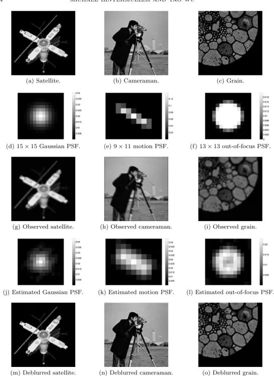
τ= 2×10⁻⁵ and the initial PSFh1to be the discrete Dirac delta function. Our experiments are performed on three different pairs of images and PSFs, namely Gaussian blur on the “Satellite” image, motion blur on the “Cameraman” image, and out-of-focus blur on the “Grain” image. In Figure1, the ground-truth
images are displayed in (a)–(c), the underlying PSFs in (d)–(f), and the corre-sponding blurred observations in (g)–(i). The results of the bilevel-optimization calibration are shown in the last two rows: (j)–(l) for the estimated PSFs and (m)– (o) for the deblurred images from the lower-level problem. It is observed that the calibrations are reasonably good in all three cases in the sense that the calibrated PSFs resemble their true counterparts and yield the deblurred images of high visual quality.
In Figure2, we also illustrate the typical numerical behavior of Algorithm6.2in the “satellite” example. Subplot (a) records the history of the smoothing parameter γk. The objective valuesJ(uk, hk) are shown in (b), which exhibit regular decrease
along iterations. The proximity measureκk in step 4 of Algorithm 6.2, shown in
subplot (c), also behaves well.
6.2.1. Comparison with a single-level optimization approach. Here we compare our bilevel approach with a single-level alternating minimization method, in the spirit of [53, 13, 23], for calibrating PSFs. More precisely, one considers the following model: minimize Jλ(u, h) := µ 2k∇uk 2+1 2kh∗u−zk 2+αk∇uk 1,γ +λ 1 2ku−u(ref)k 2+β 2k∇hk 2 over u∈R|Ωu|, h∈Q h.
The objectiveJλ combines the upper-level and lower-level objectives in the bilevel
model with a balancing weightλ >0. Fixing λ, to obtain a numerical solution for this model, one may utilize an alternating minimization scheme [13] formulated in the following.
Algorithm 6.3(Single-level alternating minimization).
1: Initializek:= 0 andh0as the discrete Dirac delta function.
2: repeat
3: Computeuk+1:= arg minu∈R|Ωu|Jλ(u, hk).
4: Computehk+1:= arg min
h∈QhJλ(u
k+1, h).
5: Setk:=k+ 1.
6: untilsome stopping criterion is satisfied.
In Algorithm6.3, step3calls for the solution of the following optimality system:
−µ∆uk+1+hk(−·)∗(hk∗uk+1−z) +α∇>(ϕ0γ(∇uk+1)) +λ(uk+1−u(ref)) = 0, which can be carried out by a simple adaption of the semismooth Newton method in Algorithm6.1. Meanwhile, step4 corresponds to a standard quadratic programm. Thus, the computational cost of each iteration in the single-level approach roughly equals that in the bilevel approach in Algorithm6.2. We terminate Algorithm6.3 once (Jλ(uk, hk)−Jλ(uk+1, hk+1))/Jλ(uk, hk)<10−6.
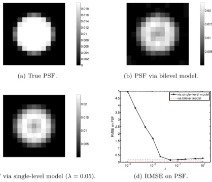
Figure3demonstrates the comparison between our bilevel approach in Algorithm 6.2 and the single-level approach in Algorithm 6.3 on the “Grain” example under exactly the same experimental setting as before. One difficulty for the single-level approach is that the proper choice of the additional weight parameter λ remains unclear. In our experiments, we have run the single-level approach with a series of differentλ’s. The resulting relative mean squared errors (RMSE) on the PSFh(λ), measured bykh(λ)−h(true)k/kh(true)k, for each λare plotted in subplot (d). The PSF via the single-level model reaches the smallest RMSE (=0.1481) whenλ= 0.05,
(a) Satellite. (b) Cameraman. (c) Grain.
(d) 15×15 Gaussian PSF. (e) 9×11 motion PSF. (f) 13×13 out-of-focus PSF.
(g) Observed satellite. (h) Observed cameraman. (i) Observed grain.
(j) Estimated Gaussian PSF. (k) Estimated motion PSF. (l) Estimated out-of-focus PSF.
(m) Deblurred satellite. (n) Deblurred cameraman. (o) Deblurred grain.
Figure 1. Calibration of point spread functions.
which is shown in subplot (c). It is observed that the bilevel model yields a PSF, see subplot (b), which is both visually and numerically (RMSE=0.1560) close to the PSF via the single-level model with the optimally chosenλ. Otherwise, the bilevel model is always superior, with respect to RMSE on PSF, over single-level models with non-optimalλ’s. Thus, our bilevel approach is favorable for its automation in
0 5 10 15 20 25 30 10−1 100 101 102 iteration γ k 0 5 10 15 20 25 30 0 0.02 0.04 0.06 0.08 0.1 0.12 iteration J ( u k, h k) 0 5 10 15 20 25 30 0 0.05 0.1 0.15 0.2 0.25 0.3 0.35 iteration κ k
(a) Smoothing parameter. (b) Objective value. (c) Proximity measure.
Figure 2. Numerical behavior.
the sense that it avoids selection of the additional parameterλwhich is often done by trail and error.
(a) True PSF. (b) PSF via bilevel model.
10−3 10−2 10−1 100 0 0.5 1 1.5 2 2.5 3 3.5 4 4.5 5 λ RMSE on PSF
via single−level model via bilevel model
(c) PSF via single-level model (λ= 0.05). (d) RMSE on PSF.
Figure 3. Comparison with single-level alternating minimization.
6.3. Multiframe blind deconvolution. Now we apply our algorithmic frame-work to multiframe blind deconvolution [6]. In this problem, the observation ~z consists of f frames, i.e. ~z = (~z1, ..., ~zf), where each frame is generated from the convolution between the source imageu(true)and a frame-varying PSF~hi over Ωh
plus some additive Gaussian noise~ηi, i.e. ~
zi=~hi∗u(true)+η~i, ∀i∈ {1,2, ..., f}.
Furthermore, each PSF~hifollows a (normalized) multivariate Gaussian distribution, i.e.~hi=h(~σi
Qθ. The parameterization of the Gaussian PSFh:Qσ×Qσ×Qθ→Qh is defined by h(σx, σy, θ) := e h(σx, σy, θ) P (jx,jy)∈Ωh e h(σx, σy, θ) (jx,jy) ,
where for all (jx, jy)∈Ωh e h(σx, σy, θ) (jx,jy) := 1 2πσxσy exp −(jxcosθ−jysinθ) 2 2(σx)2 −(jxsinθ+jycosθ) 2 2(σy)2 .
Our task is to simultaneously recover the image u(true) and the PSF parame