Structure-oriented prediction in complex networks

(1)

Structure-oriented prediction in complex networks

Zhuo-Ming Ren

a,c

, An Zeng

b,c,

*

, Yi-Cheng Zhang

c,a

a_{Alibaba Research Center for Complexity Sciences, Alibaba Business School, Hangzhou Normal University, Hangzhou 311121, China} b_{School of Systems Science, Beijing Normal University, Beijing 100875, China}

c_{Department of Physics, University of Fribourg, CH-1700 Fribourg, Switzerland}

Keywords:

Complex networks Prediction Network structure Network dynamics

Complex systems are extremely hard to predict due to its highly nonlinear interactions and rich emergent properties. Thanks to the rapid development of network science, our understanding of the structure of real complex systems and the dynamics on them has been remarkably deepened, which meanwhile largely stimulates the growth of effective prediction approaches on these systems. In this article, we aim to review different network-related prediction problems, summarize and classify relevant prediction methods, analyze their advantages and disadvantages, and point out the forefront as well as critical chal-lenges of the field.

http://doc.rero.ch

Published in "Physics Reports 750(): 1–51, 2018"

which should be cited to refer to this work.

(2)

4.1.4. Probabilistic models... 18

4.2. Link prediction in bipartite networks for recommendation... 20

4.3. Predicting salient links and extracting network backbone... 22

4.3.1. Centrality statistics... 23

4.3.2. Global thresholding methods... 23

4.3.3. Maximum spanning trees... 24

4.3.4. Extracting network backbone in bipartite networks... 25

4.4. Discovering spurious links... 26

5. Macroscopic prediction of network structure... 26

5.1. Community prediction... 26

5.1.1. Community detection... 26

5.1.2. Evolution of community structure... 27

5.2. Topological evolution... 28

5.2.1. Observation of topological evolution... 28

5.2.2. Topological evolution according to dynamics... 28

5.3. Trend prediction... 29

5.3.1. Trend prediction in online social interactions... 29

5.3.2. Trend prediction in the stock market... 30

6. Applications of prediction... 30

6.1. Prediction in biology networks... 30

6.1.1. Predicting salient nodes in biology networks... 30

6.1.2. Predicting the interaction in biology networks... 31

6.2. Prediction in scientific networks... 31

6.2.1. Predicting impact of scientific discovery... 31

6.2.2. Predicting influence of scientific researchers... 33

6.3. Prediction in economic–social networks... 35

6.3.1. Diversity and ubiquity... 35

6.3.2. Eigenvector-based complexity index... 35

6.3.3. Fitness and complexity index... 36

6.3.4. Nestedness... 36

6.3.5. Data driven methods... 37

6.4. Prediction technical–social networks... 38

7. Predictability and feedback... 39

7.1. Predictability in human behaviors... 40

7.2. Predictability in economic complexity... 41

7.3. Predictability in nonlinear dynamics... 41

7.4. Predictability in epidemics... 42

8. Summary and outlook... 42

Acknowledgments... 44

References... 44

1. Introduction

The ultimate goal of understanding a real system is to predict it. Prediction is thus always located in the core of scientific research. One can easily find the applications in various real systems such as predicting the most popular movies in online commercial systems; predicting the stock prices in financial systems; predicting the collective human dynamics in social systems; predicting the traffic congestions in transportation systems, just to name a few. However, prediction in these complex systems is particularly difficult due to their rich emergent properties and chaotic behaviors. Complex networks have been proved in the literature to be an effective tool for modeling and analyzing complex systems as they capture the intricate structure of interactions between components that lead to the complex phenomena [1]. In this context, there is a recent wave of investigating prediction problems in complex networks, aiming at not only forecasting the structural growth of the network itself but also revealing the future evolution of the dynamics taking place on the network [2]. For instance, a number of issues such as link prediction, trend prediction, human mobility prediction, information spreading prediction have been investigated.

The rapid development of the prediction research in complex networks is promoted by the accelerating availability of empirical data containing temporal information. Example includes the purchase records of online users, citations between scientific papers, instant human locations from GPS, and so on. However, the highly complex mechanisms behind these data bring in new challenge for prediction. Traditional simple methods such as polynomial regression and linear extrapolation are no longer effective. To extract accurate predictors from the empirical data, theories and methods based on statistical physics play a critical role. For instance, the mechanistic models combining multiple factors accurately predict the future citations of papers and authors [3,4]; the anisotropic rescaling of the distributions of human travel at different scales results in a statistically self-consistent microscopic model that accurately predicts individual human mobility [5]; Classic percolation

(3)

theory is employed to predict the spreading of virus or information in social networks [6,7]. Numerous such methods were developed in recent literature. Thereupon, the review will cover a wide range of topics including predictions of network structures; predictions at microscopic and macroscopic levels; theoretical analysis of predictability and practical application of the prediction tools. In this review, besides survey the simple summarization of the prediction tools, we aim to classify methods according to their relations; quantitatively compare the effectiveness of reviewed algorithms; and discuss the underlying mechanisms that cause their advantage and disadvantage. The review will be useful as a guide for the practical use of the recently developed prediction tools. Additionally, it will be meaningful for future theoretical research as it will point out the forefront as well as the standing challenges of this field.

2. Framework of prediction in complex networks

2.1. Primary issues

When speaking about prediction, people usually refer to forecasting the future based on the historical data. However, prediction is actually much broader concept. It also includes unveiling and quantifying the correlation between variables of a system, such that one variable is called a ‘‘predictor’’ of another. In addition, if certain components of a system are hidden or missing, one can also ‘‘predict’’ them by pointing out which part they are. Generally speaking, prediction in science is a study focusing on uncertain events.

Real systems are highly complex in structure and constantly evolving, prediction thus is a particular challenging task. Prediction has wide applications in a variety of real systems. A typical example is the online commercial system where an accurate prediction of the most popular products will enable the online retailers better manage their inventory. Similarly, identifying the potential young researchers allow administrator decides who to hire and to whom the fundings should be given to. The benefit of accurate prediction in stock market is even more straightforward. Due to wide applications, large effort has been devoted to design prediction tools for various real systems. Numerous classic methods based on regression and machine learning have been developed by computer scientists and researchers from specific fields such as economics and biology.

The past twenty years have witnessed the rapid development of network science. Many data from real systems are naturally described by complex networks. Examples include the social networks, citation networks, airline networks, international trading networks and so on. The network tools not only lead to more effective understanding of the structure of the real system, but also inspire numerous prediction methods at different levels. Compared with traditional methods, the related works on prediction in complex networks have their own features which can be summarized into the following six aspects.

•

Mechanistic models.Though the regression and machine learning methods are widely adopted, their prediction accuracy to some specific problems are not satisfactory as the prediction up-limit is constrained by the mis-chosen formulate. A mechanistic model, on the other hand, is constructed with the driving mechanisms of the system inferred from the historical data. Such models usually can significantly improve the prediction accuracy of the system’s future evolution.

•

Reliability.A well-performed prediction method should have both high accuracy and reliability. The data quality of real systems are not always guaranteed. In some case, the data can be overly sparse such that the method should be able to solve the cold-start problem. Moreover, the prediction has to be conducted in noisy environment where the observed data contains spurious information.

•

Bringing macroscopic and microscopic. In complex systems, collective behaviors are emerged from the local interactions. Therefore, the macroscopic-level prediction can be achieved by aggregating the prediction at microscopic level in a non-trivial way. Such approach usually has high ability in identifying potential components.

•

Predictability.Much effort in the literature has been devoted to improve the prediction accuracy. However, the up-limit of the accuracy in numerous real systems are bounded by the predictability. Therefore, knowing the theoretical predictability of a system is crucial for designing prediction methods.

•

Feedback.The prediction in some cases may have feedback effect on the evolution of the system. This is because the system may react to the information from prediction. Typical examples are the recommender systems where the recommendation may guide users’ selection by predicting what they may be interested in, and the stock market where people may purchase the stock whose price is predicted to go up.

2.2. Basic procedures

Prediction is a highly data-driven science. Data from real systems with time information are commonly used to examine the effectiveness of the prediction methods. Usually, the data from real systems are divided into a training setET_{and a probe}

setEP_{according to time.}_ET_{is regarded as the known information and the prediction algorithms run on it.}_EP_{, on the other}

hand, is treated as unknown information and used to measure the prediction accuracy after the prediction is made. To ensure the prediction methods have sufficient data to extract valuable information for prediction, the size ofET_{is usually rather}

large. However, the size ofET_{in some works are deliberately decreased to simulate the cold-start problem. The size of}_EP_is

(4)

usually small. Altering the size ofEP_{has another interpretation. A small}_EP_{is corresponding to predicting the shorter future,}

while a largeEP_{is corresponding to long term prediction. The typical size ratios for}_ET_and_EP_{are 90% and 10%, respectively.}

In some cases where the time information of the data is not available, the real data are sometimes divided intoET _and_EP

randomly.

In prediction, a method with more parameters may seem to have higher accuracy than a method with fewer parameters. However, it is very important to examine whether the seemingly high accuracy is truly due to the advantage of the method or just a result of over-fitting. A prediction method that has been over-fitted is very sensitive to minor fluctuations in the training data. An easy procedure to examine over-fitting is through a three-fold data division. Instead of dividing the data into a training setET_{and a probe set}_EP_{, the real data are divided into three subsets, i.e. a training set}_ET_{, a learning set}_EL

and a probe setEP_{. Both}_ET_and_EL_{are treated as known information,}_EL_{is used to estimate the optimal parameters which}

are finally used to predictEL_{. The accuracy in predicting}_EL_{is the final performance of the method.}

To investigate the feedback effect of a prediction method, the predicted results (denoted by a setER_{) can be added to}

ET_{to simulate the situation that the system adopts the prediction or approaches to the prediction in its future evolution.}

ET

∪

_ER_{is then compared with the real case}_ET

∪

_EP_{to reveal the influence of prediction on the evolution of the system. This}

approach is especially important for prediction in online systems. For instance, how the recommendation algorithms and search engines affect the popularity of online items. In this case, one can even make a more realistic assumption that only a fraction of the prediction results are adopted by the system and investigate how this faction influence the future evolution of the system. In addition, this approach is also used to examine the network reconstruction performance when the prediction methods are applied to recover missing data.

The data division framework is universal for most of issues for prediction. For instance, the prediction of dynamics such as spreading and cascading failure can be investigated via this framework. The dynamical processes are run until they reach stationary states in networks. The simulation time series data can also divided into aET_and_EP_{to estimate the accuracy of}

prediction methods.

2.3. Evaluation metrics

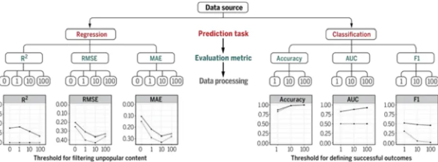
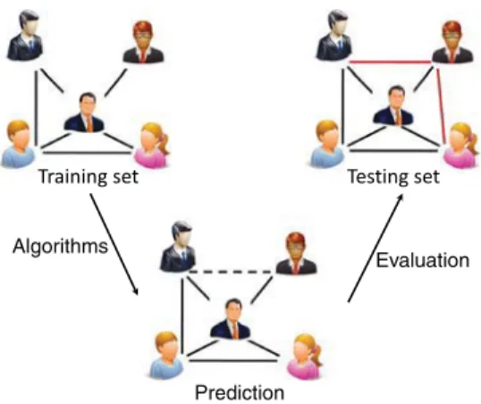
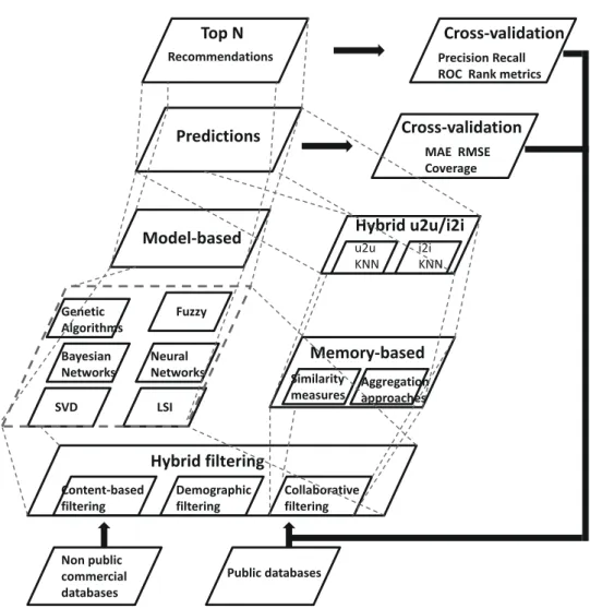
Prediction needs to be validated. Even though there are numerous evaluation metrics for prediction, one has to choose the most proper ones according to different context. Hofman et al. [8] introduced a basic procedure as shown inFig. 1. In this subsection, we will introduce several most basic and commonly used metrics for prediction evaluation. Some other metrics for specific prediction problems, we will introduce them in the corresponding sections.

Classification metrics.Numerous prediction problems are binary classification type problems, namely to distinguish what will truly happen from all possibilities. Therefore, the classification metrics in statistics are employed to measure the accuracy of the prediction methods. Within this framework, thetrue positive(TP) measures the number of real future events that are correctly predicted. Thetrue negative(TN) focus on the events that are not happening in the future and computes the number of such events that are not included in the prediction. When making predictions, it is possible to fall into two different kinds of error: predicting events that will not happen in the future (known as the type I error); and not predicting events that will happen in the future (known as the type II error). The number of type I and type II errors are respectively denoted as thefalse positive(FP) andfalse negative(FN). These quantitative are further used to design the accuracy metrics calledsensitivityandspecificity. The sensitivity reflects the ability of the prediction method in avoiding false positives, which can be written asTN

/

(TN

+

FP) in mathematical form. The specificity represents the ability of the prediction method in avoiding false negative, which is simply computed asTP

/

(TP

+

FN). A well-performed prediction method is expected to have both high sensitivity and specificity.

Area under the receiver operating characteristic curve.The receiver operating characteristic (ROC) curve is created by plotting the true positive rate (TPR) against the false positive rate (FPR) at various threshold settings. When using normalized units, the area under the ROC curve (AUC) is equal to the probability that a predictor can rank a real future eventerhigher

than a randomly chosen eventecthat will not happen in the future. It can be simply calculated as

AUC

=

∞

−∞

(TPR(T)

−

FPR(T))dT

,

(1)

whereTis the threshold. AUC ranges from [0, 1].AUC

=

1 represents a perfect prediction, whileAUC

=

0

.

5 is the result of random guessing, representing a worthless prediction.

AUC index can also be approximated in a less computational consuming way. The basic idea is to conduct in totalntimes of comparisons to directly estimate the probability thateris ranked higher thanec. If, amongntimes of comparisons,eris

ranked higher thanecforn1times and they are with the same rank forn2times, then AUC can be estimated by AUC

=

n1

+

n2

/

2

n

.

(2)

This approximation is usually used in the link prediction problem where directly computing AUC is overly time-consuming. Precision and recall.Precision and recall are another type of notable metrics in the literature. In information retrieval, precision and recall are usually defined based onTP,FPandFN. Specifically, precision is calculated asTP

/

(TP

+

FP) while recall is calculated asTP

/

(TP

+

FN) (the same as sensitivity). These two measures are both independent ofTN, which is generally

(5)

Fig. 1. Basic process of prediction.R2_{is coefficient of determination; AUC is area under the ROC curve; RMSE is root mean squared error; MAE is mean}

absolute error; F1 score is the harmonic mean of precision and recall. After [8].

unknown and much large in number. Precision and recall have other variants. One important variant is in recommender system where the calculations need to take into account the length of the recommendation list. This variant will be discussed in the corresponding section.

Correlation coefficients. In some problems, the accuracy of a prediction method is estimated by computing the correlation coefficients between the predictor and the variable that needs to be predicted. A high correlation naturally indicates a high accuracy. A typical example is predicting the spreading ability of a node in complex networks with the topological induces. There are three mainstream correlation coefficients, i.e. Pearson coefficient, Spearman coefficient and Kendal’s tau coefficient. The Pearson correlation coefficient is defined for two paired sequences (Xi

,

Yi) with lengthN.

Mathematically, it computed as rp

=

N i=1(Xi

− ¯

X)(Yi

− ¯

Y)

N i=1(Xi

− ¯

X)2

N i=1(Yi

− ¯

Y)2

,

(3)

whereX

¯

andY

¯

are respectively the mean value of the sequencesXandY.rpranges from

−

1 to 1, with

−

1 and 1 respectively

indicating a completely negative and positive correlations. Though the Pearson coefficient is widely used, it has a obvious drawback. It is very sensitive to extreme values inXandY. As the heavy-tailed distributions are found in numerous systems, this drawback cannot be neglected.

The second coefficient is the Spearman coefficient. It is defined for the ranks of sequencesXandY. Denotingxiandyi

respectively as the ranks for the componentsXiandYi, the Spearman coefficient can be written as

rs

=

N i=1(xi

− ¯

x)(yi

− ¯

y)

N i=1(xi

− ¯

x)2

Ni=1(yi

− ¯

y)2

.

(4)

Apparently, the Spearman coefficient is the Pearson coefficient of the ranks of two sequencesX and Y. It reflects the monotonic relatedness of two sequences. There is a simple way to calculate Spearman coefficient as

rs

=

1

−

6

N_i₌₁(xi

−

yi)2

N(N2

−

₁₎

.

(5)

The Kendal’s tau coefficient also measures the rank correlation between two sequencesXandY. Specifically, it counts the difference between the number of concordant pairs and the number of discordant pairs between these two sequences. The formula reads

τ

=

N i=1

N j=1sgn

[

(xi

−

xj)(yi

−

yj)

]

N(N

−

1)

,

(6)

wheresgn(x) is the sign function, which returns 1 ifx

>

0; 1 ifx

<

0; and 0 forx

=

0.

τ

value also ranges between

−

1 and 1. As Kendal’s tau requires a large number of pair comparison, its computational complexity is higher than the previous two coefficients.

3. Node-oriented microscopic prediction of network structure

In the literature, a mathematical framework is proposed for predicting the properties of individual based on the scale of complex systems. Kleiber’s law suggests that for the majority of animals, the 0.75 power of body mass is the most reliable basis for predicting the ratio of metabolism [9]. West’s observation also summaries similar scaling prediction in quantity arising from complex systems [10]. As the big data era comes, powerful computers made it possible to analyze data for complex systems containing a large number of components: from man-made systems and social systems such as the World

(6)

Table 1

Linear and nonlinear growth mechanisms. HereP(k) is degree distribution.

Name (i) P(k) Ref. Preferential attachment ∝ki k−3 [12] Asymptotically linear ∝aki k−γ γ→2 ifa→∞ γ→∞ifa→0 [13] Asymptotically linear ∝b+ki k−γ _γ_→ 2 ifb=0 γ→∞ifb→∞ [14,15]

Multiplicative node fitness ∝ηikia ∼k−

1−C ln(k) [16] Additive–multiplicative fitness ∝ηi(ki−1)+ςi ∼k −1−m ln(k);(m∈ [1,2]) [16] Nonlinear ∝kα_i – [13]

a_{If give a uniform fitness distribution and}_C₌₁_._255.

Wide Web and the Internet, online social networks, networks of movie actors, scientific collaboration networks, epidemic networks, and the sex web to biological systems such as the metabolic network, protein interaction networks, cell-signaling and food webs. In general, the complex networks consist of nodes that interact with each other, so that the interactions have both some level of regularity and randomness. We will introduce node-oriented microscopic prediction of network structure. In this subsection, the content includes model-based node degree prediction, extrapolation-based node popularity prediction, node influence prediction, and discovering the hidden nodes.

3.1. Model-based node degree prediction

One of the basic assumptions of evolving network models is that the total number of links in a growing network is a linear function of the network size, that is, of the total number of nodes. This linear growth does not change the mean degree (i.e. the number of connections per nodes) of the network. Besides, there are also growth models with asymptotically linear or node attributes extend the research. However, in many real growing networks, the node degree evolves with time. The recent works take into account the temporal effects of the network growth. The framework of a simple growing network can be described that at timet

+

1 a new node is introduced to connect to an existing nodeiwith the probability

(i) and the node

ihasklinks before timeti.e. degree. It predicts a strong relationship between a node’s age and its degree. In this subsection, we mainly classify related works into degree prediction without aging effects and with aging effects.

3.1.1. Network growth models without aging effects

We first introduce several classic network generation models. In a random network like classic Erdős–Rényi (ER) model [11], a node is introduced to connect to another nodeiwith a constant probability

(i)

=

p (0

≤

p

≤

1), and thus the degree distribution follows Poisson. In small world networks, each link is rewired to connect two randomly selected nodes with a constant probability

(i)

=

p(0

≤

p

≤

1) and finally, degree distribution also follows Poisson. However, the empirical results from real networks show that these real networks are growing with new nodes added to the existing networks, and finally the degree of the network follows power-law, as opposed to the Gaussian or Poisson degree distributions of random networks. The famous model for the growth of networks with the mechanism called preferential linking, for instance the Barabasi–Albert model [12]. Mathematically,

(i)

∝

k. Thus, this linear type of growth is usually considered to be a natural feature of growing networks, and is a basis of other linear and nonlinear growth as

(i)

=

b

+

akα, seeTable 1.

3.1.2. Degree growth with aging effects

Despite the preferential attachment provides a common framework for many theoretical models and empirical data sets, it neglects the temporal effects of network growth. Many real systems display the number of links increases faster than the number of nodes, thus the increase of the average degree in growing network describes the corresponding scaling relations for the accelerated growth. If one considers constant initial attractivenessbin directed networks [15], at timeta new node is added and points to a number of random nodes in the network. Additionally there arec0tθ links are generated and each node is directed to a higher in-degree nodesiwith asymptotically linear preferential attachment

(kin)

∝

b

+

kin. The

average degree of network is k

∼

tθ and the corresponding degree distribution isP(k)

=

k−γ, here

γ

=

1

.

5 if

θ

→

1, and

γ

→

2 if

θ

→

0. If one considers internal links with a probability [17], the average degree of network is k

=

at

+

2band corresponding degree distribution also preserves power-law form.

In another model, new nodes are added to the network with a constant probability, and the selected nodes connect tobexisting nodes in the network with preferential attachment (

(i)

∝

bki). Additionally, the numberaN(t) of links is a

percentageaof the nodesN(t) that are present in the network are chosen. The probability that a link connects nodesiandjis expressed as

∝

aN(t)kikj. As a result, the average degree of the network is k

=

at

+

2bbut the power-law degree distribution

displays a segmentation at a critical degree. In addition, in some systems, the probability that a new node connects to a nodei

is not only proportional to the degreeki, but also depends on its age. In the gradual aging model [15], a new node is introduced

(7)

to connect to an existing nodeiwith the probability

(i)

∝

ki(t

−

ti)−v, where

v

is a tunable parameter,tiis the age of node

i. The observation of empirical data sets reveals papers and actors gradually lose their ability to attract more citation and collaboration.

In the mentioned methods, if the degree growth of an observed network is agreed with a proposed model, one can use the model to fit the real degree growth and then use the model to predict the future degree. But usually, the degree growth of real networks deviate from these proposed models. Medo et al. [18] proposed a fitness model for growing networks based on the empirical observations. A new node at timetis introduced to connect to an existing nodeiwith the probability

(i

,

t)

=

_tki(t)Ri(t)

j=1kj(t)Rj(t)

.

(7)

HereRi(t) is the relevance of nodejat timet which is can be observed in the real network. According to the preferential

attachment (PA), the temporal degree that the nodeiowned at timet

+

Δt is predicted byΔki(t

+

Δt)(PA)

=

ΔL(t

+

Δt)ki(t)

/

L(t), whereΔL(t

+

Δt) is the number of links added to the network duringΔt,L(t) is the number of cumulated

links at timet. If, in the reality, the nodeiactually owns the degreeΔki(t

+

Δt) duringΔt, the relevance can be defined as

the ratio between the actual and the expected degree duringΔt,

Ri(t

,

Δt)

=

Δ ki(t

+

Δt) Δki(t

+

Δt)(PA)

=

Δki(t

+

Δt)L(t) ki(t)ΔL(t

+

Δt)

.

(8) Ren et al. [19] used the relevance model in the bipartite networks to characterize how the popularity of online contents evolved over time, and found that the popularity of the online contents typically exceeded theoretical preferential popularity (Ri

1) in the early lifespan, and later restricted to the classic preferential popularity increase mechanism (Ri

≈

1).

3.2. Extrapolation-based node popularity prediction

The large number of online contents including video, photo, music sharing, blogs, wikis, social bookmarking, collaborative portals, and news aggregators highlight the challenge of predicting how much attention any of it will finally attract. Thus, predicting the popularity of the online contents not only deepens our understanding of complex systems but also has significant implications for marketing and traffic control to policy-making and risk management. The database of online contents’ past history produces a big amount of time-stamped data, making it possible to study the dynamics of the online popularity and how it evolves over time on a global scale [20,21].

Predicting the popularity has been widely studied in the literature focusing on videos [22,23], music [24], news [25], and other online social collective dynamics [26]. Cha et al. [27] observed a highly linear correlation between the number of video views on early days and later days on YouTube. Borghol et al. [28] suggested that a strong linear growth law is the most important factor of prediction of popularity [29]. Shen et al. [30] used the reinforcement Poisson mechanism based on the well-known ‘‘rich-get-richer’’ phenomenon to predict the popularity dynamics. Instead of a stronger presence of the rich-get-richer phenomenon, Vasconcelos et al. [31] showed a lower correlation between the early and late popularities in Foursquare. Chen et al. [32] took the view of video popularity lifespan and found that the relative popularity of the online content is dependent on its age and its intrinsic attributes.

Furthermore, the prediction of popularity is by no means restricted to ‘‘rich-get-richer’’ behaviors, and should take into account the exogenous attributes of the online contexts [33]. Accordingly, Ratkiewicz et al. [34] examined the popularity of Wikipedia topics and Web pages and presented an evolving model that combines the classic preferential growth mechanism with the influence of exogenous factors. The exogenous attributes are incorporated in modeling and predicting evolving popularity dynamics in user-generated videos [35], the citation of scientific release [18,36], and the activity of scientists [37]. In addition, there are also some novel prediction approaches for item popularity like considering local clustering behavior of users [38] and using machine learning techniques to explore item attributes in different dimensions [39]. In this subsection, we will review some typical prediction methods of item popularity based on ‘‘rich-get-richer’’ mechanism and item attributes.

3.2.1. Linear models

The very popular items are thought to result from a positive feedback mechanism leading to rich-get-richer. Motived by this, Szabo et al. [40] proposed a linear model to predict the popularity. At first, one can give two definitions. Reference time

tr is the time at which they intend to predict the popularity of an item whose age with respect to its upload (promotion)

time. Indicator timetiis that when in the life cycle of the item they performed the prediction (ti

<

tr). Thus, the linear model

is proposed as,

lnN(tr)

=

ln

[

r(ti

,

tr)N(ti)

] +

ξ

(ti

,

tr)

=

lnr(ti

,

tr)

+

lnN(ti)

+

ξ

(ti

,

tr)

,

(9) whereN(t) is the popularity of the item at timet.r(ti

,

tr) accounts for the linear relationship between the log-transformed

popularities at different times.

ζ

is a noise term describing the randomness one can observed in the data. There is also an

(8)

alternative description for the observed correlations: lettivary in the model, the popularity at the given timetrshould be

described by the following formula, lnN(tr)

=

lnN(t0)

+

tr

τ=t0

η

(

τ

)

,

(10)

η

(

τ

) is the noise following an arbitrary, fixed distribution, and

τ

is taken in small, discrete time steps.t0is an early point in time after the birth time of an item.

3.2.2. Weighted linear models

Preferential attachment is a well-known mechanism of the linear growth law which assumes that the probability a node to attract a new link is proportional to its cumulative degree. Zeng et al. [41] considered that items which are popular at time

tare expected to have better chances to become more popular. This implies that the cumulative degree of an itemk_α(t) and Δk_α(t) is a great predictor of its future popularity increase. Mathematically, the prediction of the popularity of a given target item

α

,

s_α(t

,

Tp)

=

(1

−

λ

)kα(t)

+

λ

Δkα(t

,

Tp)

=

k_α(t)

−

λ

k_α(t

−

Tp)

;

(11) When

λ

=

0, the predictor simplifies to the total popularity method; When

λ

=

1, the prediction equals to the recent popularity. The method can be extended to the weighted popularity prediction in the bipartite networks as the following form,

s_α(t∗

,

Tp)

=

i

(Aiα(t∗)

−

Aiα(t∗

−

Tp))ki(t∗)γ

.

(12)

HereAiαis the interaction between an item

α

and a useriin a bipartite network, for example, in a rating system, a useri

rate 5-stars to a movie

α

.

γ

is a weight parameter which quantifies the activeness of users. If it is extended to the user social network,ki(t∗) can transform to the influence of useriasIi. In addition, one can consider the mechanism that the influence

of a link exponentially decays with time [42]. An aging function is accordingly introduced to calculate the prediction of popularity as,

s_α(t)

=

i

Aiα(t)eγ(Tiα−t)

,

(13)

whereTiαdenotes the time at which useriselected an item

α

.

γ

is a positive parameter which controls the decay speed. A

larger

γ

indicates a faster decay, and

γ

=

0 corresponds to the cumulative popularity without any decay.

3.2.3. Reinforced Poisson models

Shen et al. [30] proposed a generative stochastic framework applying a reinforced Poisson process to predict the item popularity. The reinforced Poisson process takes account three important factors: (1) Fitness of an item which can characterize its intrinsic competitiveness against other items; (2) The relaxation function corresponds to the aging effect on the ability to attract new attention; (3) A reinforcement mechanism according to the well-known rich-get-richer phenomenon. Taking a citation network as an example, and the reinforced Poisson process is defined as the rate function

x(t) for a given paper,

x(t)

=

λ

k(t)f(t

;

θ

)

,

(14)

where

λ

is the fitness of a paper,k(t) is the total number of citations received until timet,f(t

;

θ

) is the relaxation function that characterizes the ability to attract new attention which affected by the aging parameters

θ

. Consider the aging of papers and assume a log-normal relaxation function in citation network as well as in other online contents, one can obtain,

f(t

;

μ, σ

)

=

√

1

2

πσ

t exp(

−

(lnt

−

μ

)

2

σ

2 )

.

(15)

The parameters

μ

and

σ

can be calculated by maximizing the logarithmic likelihood.

3.2.4. Self-avoiding mass diffusion models

Zeng et al. [43] devised a self-avoiding mass diffusion (SAMD) method which outperformed extrapolation in the long run and predicted future popular items long before they become prominent. It is noted that the diffusion processes have been applied to design the recommendation algorithms which can be regarded as a prediction problem [44–47]. Consider a bipartite networkAiαbuilt by the interaction between an item

α

and a useri, the initial condition and the diffusion processes

is modified as follows:

(9)

(1) The initial condition is asm(_iα)(0)

=

aiα(t)

−

aiα(t

−

Th).

(2) The diffusion process is from a user to a user only considered connections between time (t

−

Th) andt, thus, the

diffusion function is defined as,

W_ij(t

,

Th)

=

1

−

δ

ij Δki(t

−

Th

;

t) Z

β=1 Δaiβ(t

−

Th

;

t)Δajβ(t

−

Th

;

t) Δk_β(t

−

Th

;

t)

;

(16) whereΔajβ(t

−

Th

;

t)=ajβ(t)-ajβ(t

−

Th) andΔki(t

−

Th

;

t)=ki(t)-ki(t

−

Th). sincet

≥

t

−

Th,Δki(t

−

Th

;

t) andΔkβ(t

−

Th

;

t)

more than 0. Finally, the predicted ranking of popular items is given by

s_α(t

,

Tf

,

Th)

=

rank(M ₍_α₎ (t

,

Th))

;

(17) M(α)(t

,

Th)

=

N

i Δa(t

−

Th

;

t)m ₍_α₎ i (1)

;

(18)

m_i(α)(1)

=

W(t

,

Th)

·

m ₍_α₎ i (0)

.

(19)

The higher the diffusion score, the more similar are the users who have already collected item

α

. Thus, the item could have higher popularity.

3.3. Predicting the influence of nodes

Recently, more and more attention has been paid to predicting individual influence in networks. With an effective algorithm to predicting spreader influence [48–50], we can, for instance, hinder spreading in the case of diseases or accelerate spreading in the case of information dissemination. This problem can be interpreted as predicting the spreading influence of nodes based on its structural properties.

So far, various centrality measures have been applied to predict or identify the node of influence in complex networks. Related classical centrality measures include the degree as the number of neighbors a node connects with, the closeness centrality [51] as the reciprocal of the sum of the geodesic distances to all other nodes, betweenness centrality [52] as the number of shortest paths through a certain node, eigenvector centrality [53] as the component of the eigenvector to the largest eigenvalue of the adjacency matrix, k-shell [54] as the node location in a network.

Lately, a lot of works try to design efficient algorithms that outperform the classical centrality methods. For example, some algorithms focus on directly modifying the basic centrality measures including degree [55], closeness, and between-ness [56,57]. Some works focus on improving the k-shell method by removing the degeneracy of the method [58,59]. Some others try to cut down the computational complexity of eigenvector [60]. Moreover, the concept of path diversity is used to improve the ranking of spreaders [61]. Some methods are also designed in directed networks to identify the influential nodes such as LeaderRank, which is shown to outperform the well-known PageRank method in both effectiveness and robustness [62]. Reviews [48,49] introduced methods in identifying and predicting vital nodes and compared well-known methods on disparate real networks. Another review [50] surveyed the existing methods in ranking nodes of both static and evolving networks.

In real life, many networks are inherently evolving. For example, friends are added and removed in online social networks; the topology of the Internet changes with time; and contacts between mobile devices depend on the time of day. Ghoshal et al. [63] observed that PageRank ranking is sensitive to topological perturbation in random networks. In contrast, in scale-free networks the emergence of super-stable nodes whose ranking becomes independent of perturbations, which due to the fat-tailed nature of the degree distribution. Thus, the classical or extended centralities could manifest different spreader topology in a network, which leads to different efficacy and applicability for identifying vital nodes and predicting the influence of spreaders [64].

In this subsection, we first discuss the effect of tunable network topology on the accuracy of the four centrality methods for predicting the node of significance or influence in undirected networks, then introduce solutions for the dynamical networks with tunable network topology and the complexity of computation in large-scale networks. Finally, we review the age bias of metrics on predicting the node significance in directed growing networks and will introduce predictability of scientific discovery.

3.3.1. Influence of nodes in dynamic networks

Normally, an undirected networkG

=

(V

,

E) withN nodes andMlinks could be represented by an adjacent matrix A

= {

aij

} ∈

Rn,n, whereaij

=

1 (i

=

j) if nodeiand nodejare connected, andaij

=

0 otherwise. Many topology measures

have been proposed to identify the node influence. Here we introduce the procedure of identifying the influence of nodes in undirected networks for simplicity. The topology measurements will generate a ranking list of nodes. In principle, the ranking from an effective ranking method should be as close as possible to the ranking based on the real spreading process. one can employ spreading model to simulate the spreading process on networks such as the susceptible–infected–recovered (SIR) model [65]. In the SIR model, all nodes are regarded as initially susceptible except one infectious node. At each step,

(10)

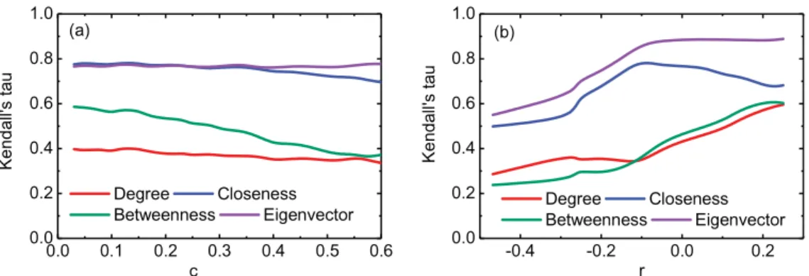
Fig. 2.Tunable network topology affects accuracy of node centrality. (a) Variation of centrality measures accuracy with different clustering coefficient in HK model. (b) The accuracy analysis of four centrality methods on the scale-free network model with tunable assortative coefficientr.

the infected nodes will spread the virus to susceptible neighbors with a certain infectious rate (

β

), and an infected node will recover after a few spreading steps. The spreading influence of nodeiis denoted asS_iβ, which is quantified in terms of the total prevalence of the epidemic process, i.e. the fraction of nodes being infected when the infection starts at nodei. Based on this, one could obtain the true spreading influence of nodes and a corresponding ranking can be generated by the topology measures. Kendall’s tau coefficient

τ

[66] is used to measure the correlation between the topology-based ranking and the spreading-based ranking. A higher Kendall’s tau value

τ

indicates a more accurate identification of the nodes’ spreading influence. Node centrality measurements are based on characterizing the network topology structure in a certain perspective. Actually, the real networks are evolving with time, the evolution of the network topology structure would affect the accuracy of the node centrality. Thus, we investigate the performance of centrality methods for a growing scale-free network model with tunable network topology structure.

We first discuss effects of tunable network clustering and employ the Holme–Kim model [67] to construct scale-free networks with tunable clustering. The HK (Holme–Kim) model is introduced as follows, (1) Preferential attachment (PA). The newly added node connects to the existing nodeipreferentially, which is described as the same as the preferential attachment. (2) Triad formation (TF): If a link betweenjandiwas added in the previous PA step, then add one more edge fromjto a randomly chosen neighbor ofiwith a probability.

For comparing with the accuracy of the four centrality measures, we simulate the susceptible–infected–recovered (SIR) spreading on the tunable clustering networks and calculate the accuracy as the correlation between the centrality value of nodes and their spreading coverage in the network with SIR model.Fig. 2a shows that degree centrality and the betweenness centrality are more accurate in networks with lower clustering, while the eigenvector centrality performs well in high clustering networks, and the accuracy of the closeness centrality keeps stable in networks with tunable clustering. In addition, the accuracy of the degree centrality and the betweenness centrality are more reliable in the spreading process with the high infectious rates than that of the eigenvector centrality and the closeness centrality.

We also investigate the performance of centrality methods for a growing scale-free network model with tunable assortative coefficient [68]. This network model (namely TASF model) is defined as: (1) The newly added node connects to the existing nodeipreferentially, which is described as the same as BA model; (2) This node selects a neighbor nodes

of the nodeiwith probabilitykα(i)

/

_j_∈_Γ ik

α₍_j_{), where}

α

_{is the tunable parameter and}_Γ_i_{is the neighbor node set of node} i. The accuracy in the TASF networks with positive assortative coefficient has different trend from the ones with negative assortative coefficient.Fig. 2b illustrates that the accuracy analysis of four centrality methods on the scale-free network model with tunable assortative coefficientrand different infectious rate

β

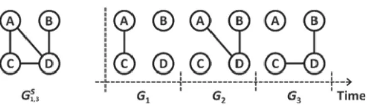
. One can find that when the network changes from disassortative to assortative, i.e. value ofrfrom negative to positive, the accuracy of the degree centrality and the betweenness centrality trends to be larger, but different of the eigenvector centrality and the closeness centrality, whose accuracy at first increases to peak point and then descends. In summary, the assortative coefficient presenting degree–degree correlation significantly influences the accuracy of centrality.

In addition, one can find that the traditional centrality methods are by no means easy to be applied to predict node influence in the dynamic networks. Many real networks are an inherently evolving, and the structure of the network operates affects the performance of prediction. Therefore, it is necessary to introduce methods to predict node influence in dynamic networks. A dynamic network can be represented as a series of static networks in each period. As revealed inFig. 3, the problem for predicting the average network centrality values of the nodes is as follows: a dynamic network can be observed duringkpast time intervals and indicated asG1,k, theGk+l,k+l+mwill a network in future and be unknown now.

A reasonable solution is to use the average centrality value duringkpast time intervals to predict the average centrality of nodes in the futureGk+l,k+l+m. Kim et al. [69] designed a prediction function. Assume the past networkG1,k, and time

windowslandm(k

<

l

<

m), the problem can be formulated on minimizing the predicted centrality and true centrality by using Polynomial Regression. With this notation, the problem is transformed to minimize the average error between the

(11)

Fig. 3.An example of the dynamic network. (Left) aggregated static network. (Right) time-varying dynamic network. After [69].

guessed centrality values and the true centrality values. GiveGD₁_,_k,landm, one can findC

˜

a,b(u) wherea

=

k

+

l,b

=

a

+

(m

−

1)

for eachu

∈

Vto minimize,

Error(GD₁_,_k

,

l

,

m)

=

u∈V

|

Ca,b(u)

− ˜

Ca,b(u)

|

V

|

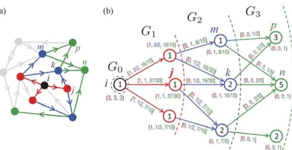
(20)

There also exists challenging situation that complex networks would contain millions of nodes and links. Some methods such as closeness and betweenness could better quantify the influence of a node, but they have higher computational complexity due to calculating the shortest paths between all pairs of nodes in a network. Fortunately, one does not need to compute accurately the total centrality, the proposed range-limited betweenness centrality [70,71] can predict betweenness centralities of individual nodes and even have an overlap of 75% for top 100 nodes with betweenness centrality. For the root nodei, the initial condition is that

σ

ii

=

1 for other nodes,k

=

i, one can set the

σ

ik

=

0. The following steps are repeated

for eachL-range subnetwork,l

=

1

, . . . ,

L. The detailed steps are as follows, and an example of the calculation is also shown inFig. 4.

(1) Build subnetworkGl(i) using breadth-first search.

(2) Calculate

σ

ikfor all nodesk

∈

Gl(i) using

σ

ik

=

j

∈

Gl−1(i) (j

,

k)

∈

Gl(i)

σ

ij

,

(21) and setbl_l(i

|

k)

=

1.

(3) Proceed backward throughr

=

l

−

1

, . . . ,

1

,

0

.

At first calculate thel

−

BCsof links (j

,

k)

∈

Gr+1(i) (j

∈

Gr(i),k

∈

Gr+1(i)) recursively;

br_l+1(i

|

j

,

k)

=

br_l+1(i

|

k)

σ

ij

σ

ik

.

(22) For nodesj

∈

Gr(i), one can use above equation and get

b_lr(i

|

j)

=

b_lr+1(i

|

j

,

k) (23)

(4) Finally return to step 1 until the last sub cellGL(i) is reached. At the end, the cumulative

[

l

] −

BCs, that is the

BL(i)

=

l=1Bl(i).

In many real cases such as advertising and news propagation, the spreading only aims to cover a specific group of nodes. Therefore, it is necessary to study the spreading influence of nodes toward localized targets in complex networks. A reversed local path algorithm [72] is devised for this problem. The basic idea is inspired by computing the paths up to length 3 starting from the target nodes to other nodes. The paths with different lengths are aggregated to obtain the final ranking score of a node. Mathematically, IRLP

=

2

l=0

f Aijl+1

,

(24)

wherefis a 1

×

Nvector in which the components corresponding to the target nodes are 1, and 0 otherwise.Ais theN

×

N

adjacency matrix of the networkAij. Here,

is a tunable parameter controlling the weight of the paths with different lengths

and is set to be a small value.

3.3.2. Significance of nodes in growing networks

As we know, the world overflows with creative works. In reality, it is difficult to measure the significance of works, because the evaluation of the true significance of the work depends on the historical moment, and very much ‘‘in the eye of the beholder’’. Fortunately, thanks to the big data related to the work, we can evaluate significance of the work independently according the network structure, and can predict the work who will potentially win big awards like ‘‘Oscar’’ or ‘‘Nobel’’. Many popular ranking algorithms like Google’s PageRank [73] and degree are static in nature which exhibit main

(12)

Fig. 4.The calculation of the range-limited betweenness centrality. (a) An example of toy network. The three successive shells ofC3subnetwork of nodei

are colored red, blue, green. Gray elements are not part of subnetwork. (b) Thebr

l(i|j) values are corresponding for shellsl=1,l=2, andl=3. After [71].

shortcomings when applied to real networks that rapidly evolve over time. Network-based metrics like CiteRank [74] and long gap degree [75] consider time effect. However, a fundamental question is still open: what performance of methods on uncovering significant nodes in the growing networks? Mariani et al. [76] analyzed the relationship between the algorithm’s efficacy and properties of the network and showed that realistic temporal effects make PageRank fail in individuating the most valuable nodes for a broad range of model parameters. Mariani et al. [77] also developed a rescaled PageRank centrality with the explicit requirement that paper score is not biased by paper age and identified the Milestone papers [78] and predicted significant papers [77] according to the network of citations among the 449,935 papers published by the American Physical Society (APS) journals between 1893 and 2009.

Furthermore, Medo et al. [79] introduced discoverers as the users in data from real systems who significantly outperform the others in the rate of making discoveries, i.e. in being among the first ones to collect items that eventually become very popular. Furthermore, statistical null models serve this purpose by producing random networks whilst keeping chosen network’s properties fixed. While there is increasing interest in networks that evolve in time, we still lack a robust time-aware framework to assess the statistical significance of their observed structural properties. Ren et al. [80] proposed a dynamic null model that preserves both the network’s degree sequence and the time evolution of individual nodes’ degree values. The proposed model can be used to explore the significance of widely studied network properties such as degree– degree correlations and the relations between popular node centrality metrics.

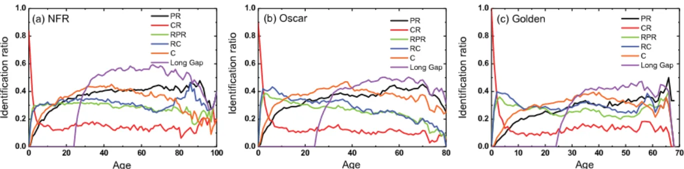
Recently, the review [50] surveyed the existing ranking algorithms, both static and time-aware, and their applications to evolving networks, and deep understanding of how existing ranking algorithms perform, and which are their possible biases that may impair their effectiveness. Simultaneously, recent advances in predicting the significance of the node in evolving networks have enabled the development of a wide and diverse range of ranking algorithms that take the temporal dimension into account. Here, this subsection will give a comparison of metrics based on network-based metrics according to a growing networks of citation between US movies, with results presented inFig. 5.

Normally, a citation networkG

=

(V

,

E

,

T) withNnodes andMlinks with time stamp could be described by an adjacent matrixA

= {

at

ij

} ∈

R

N,N_{, where}_at

ij

=

1 if nodejis cited by nodei(i.e.i

→

j) at timet, andaij

=

0 otherwise. Now, we

introduce a few well-known metrics based on network topology.

Citationsis the simplest one, which is defined as the number of times each node is cited as follows,

Ci

=

j

aij

,

(25)

where the citations could be called in-degree (kin

i ) as well. The corresponding out-degree of nodeiis defined ask out i

=

iaij.

Long GapThe formula for the time lag of a citation is as follows:

t

=

y(iout)

−

y(iin)

,

(26)

wherey(i) is an age of nodei, andiout_and_iin_{are the node on the outgoing and incoming sides of a link, respectively. After}

calculating the time lag for every link in the network, we count the number of citations with the time lag of at leasttyear that each node receives. This is the long-gap citation count [75]. It is noted thattequals 25 year in movie citation networks.

(13)

Fig. 5.The identification ratio of five metrics on different age of significant works. We only consider top 5% raking list in movie citation networks and then compute the number of significant works corresponding to their ages.

PageRankThe nodeiof PageRank [73] can be calculated as the stationary solution of the recursive formula as follows,

PRi(s)

=

1

−

d N

+

d

j aji kout j sgn(kout_j )

+

1 N(1

−

sgn(k out j ))

PRj(s

−

1)

,

(27)

wheredis damping factor, and sgn(x) is sign function. Mostlydequals 0.5 which is the usual choice for citation data [81]. CiteRankCiteRank algorithm is a time-dependent variant of PageRank with a teleportation term that decays exponen-tially with node age, which is intended to favor the recent nodes and thus provide a better representation of nodes’ relevance for the current lines of research [74]. The node of CiteRank scoresCRican be found as the stationary solution of the following

set of recursive linear equations,

CRi(s)

=

(1

−

d) exp(

−

(t

−

tj)

/τ

)

jexp(

−

(t

−

tj)

/τ

)

+

d

j aji kout_j sgn(k out j )

+

1 N(1

−

sgn(k out j ))

CRj(s

−

1)

,

(28)

wheretiis the birth date of nodeiandtis the time at which the scores are computed. We will set

τ

=

2

.

6 andd

=

0

.

5 in

movie citation networks.

Rescaled methodsTo overcome the well-known PageRank’s bias against old nodes in citation data, CiteRank algorithm introduces an exponential penalization for an old node. However, CiteRank score does not allow one to fairly compare papers of different age. The rescaled methods do not depend on paper age [82]. The rescaled methods [77] is derived from Citations and PageRank score respectively and have two steps, we take the rescaled PageRank as an example as follows,

1. Compute PageRank score for each node and label whole nodes in order of decreasing age.

2. For a nodei, the mean PageRank score

μ

i(PR), and corresponding standard deviation

δ

i(PR) calculated by the set of

nodesj

∈ [

i

−

_Δp

,

i

+

_Δp

]

which are labeled by step 1. Then, the rescaled PageRank score of nodeiis given as,

RPRi

=

PRi

−

μ

i(PR)

δ

i(PR)

,

(29) where the parameterΔprepresents the number of nodes in the averaging window of each node. It is noted that in order to have the same number of nodes in each averaging window, a different definition of the averaging window is needed for the oldest and the most recent_Δpnodes. For the oldest and the most recent nodes, one can calculate

μ

i(PR) and

δ

i(PR) over the

nodesj

∈ [

1

,

2Δp

]

andj

∈ [

N

−

2Δp

,

N

]

, respectively. Analogously, the rescaled citation can be computed by the above two steps.

In theory, the calculation of the significance of the node should be independent of the age of nodes, but the above classical or extended metrics could manifest age bias in citation networks which means that some nodes’ significance are benefit from their age. The age bias leads to different effectiveness and applicability for identifying and predicting the significance of the nodes.

We now discuss the performance of the metrics for predicting and identifying significant works in a movie citation network. Movie citation network is introduced as follows: Like scientists, artists are often influenced or inspired by prior works, for example, the famous flying bicycle scene in E.T.: The Extra-Terrestrial (1982) is similar to a sequence in The Thief of Bagdad (1924) where characters also fly in front of the moon. The movie citations come in the form of similar quotes, similar settings, or similar movie techniques and so on. Using the movie citations between movies, we can construct a directed network where a node is a movie, and a direct link is a citation. As the above example, we can build a directed link from E.T.: The Extra-Terrestrial (1982) to The Thief of Bagdad (1924). This network consists of 15,425 movies connected by 42,794 citations. The whole movies produced in the United States from 1894 to 2011. The detailed description of the movie citation network can be seen in Ref. [75].

In reality, it is difficult to measure the significance of works, because the evaluation of the true significance of the work depends on the historical moment, and very much ‘‘in the eye of the beholder’’. By definition, we select movies from NFR,

(14)

Oscar, and Golden Globe three representative awards in the USA filmdom as three significant work lists. The NFR highlights ‘‘culturally, historically, or aesthetically significant’’, and the requirement of films being released at least 10 years ago. But Oscar and Golden Globe awards are an annual American awards ceremony honoring cinematic achievements in the film industry. In addition, Oscars are awarded from a professional honorary organization, but Golden Globe awards are decided by the wide public attention.

One can consider top 5% ranking list in movie citation networks and calculate the identification ratio between the number of significant works and the works with the top ranking positions. A higher identification ratio means a higher accuracy of the metric. The age bias of metrics for identifying significant works in citation networks is revealed inFig. 5. The mechanism of their backside should be the main inducement that causes the age bias of metrics for identifying significant works in citation networks.

As we know in citation network, nodes that had been cited many times in the past were more likely to be cited again. Thus the metric of Citations naturally prefer to identifying old nodes, and Long Gap metric takes this advantage to mine hidden significance of old nodes thoroughly. Meanwhile, the famous PageRank algorithm gets to benefit from adaptive and parameter-free and then broadly uses in different areas of science. Compared to PageRank algorithm in favor of old nodes in citation networks, the CiteRank allows an exponential penalization for old nodes, and successes to properly distinguish nodes with early age groups. Further, one way of avoiding that the metric of Citations preferences to old nodes and PageRank fails in the growth of networks owing to the temporal effects, the rescaled methods directly balance age bias of the targeted metrics of Citations and PageRank. These results could give a firmer foundation for age bias of the metrics for identifying significant nodes, which have been studied extensively to describe the dynamics of real evolving networks.

3.4. Prediction of missing nodes

The approaches are used to predict the hidden nodes are either heuristic in nature [83] or rely on rules of network evolution [84]. Recent advance focuses on reconstructing the network using compressive sensing framework to uncover missing nodes in complex networks [85–91]. The basic idea is that treating the system as if there was no hidden node. The neighbors of the hidden node tend to exhibit abnormally dense interaction patterns. According to the multiple time series analysis, some nodes in comparison with those associated with normal nodes do not have hidden nodes in their neighborhoods. To detect a hidden node, it is necessary to identify its neighboring nodes. For an externally accessible node, if there is a hidden node in its neighborhood, the corresponding entry in the reconstructed adjacency matrix will exhibit an abnormally dense pattern or contain meaningless values. In addition, the estimated coefficients for the dynamical and the coupling functions of such an abnormal node typically exhibit much larger variations when different data segments are used, in comparison with those associated with normal nodes that do not have hidden nodes in their neighborhoods. The multiple time-series segments is used to calculate the variance in the reconstructed coefficient vectors for all nodes as follows.

σ

i

=

1 T T

t=1 1 N N

j=1 (

w

ij

− ˆ

w

ij)2

,

(30)

whereT is the number of data segments used in time-series analysis,Nthe network size and

w

ˆ

ijthe average weights

overT simulations. The neighboring nodes of the hidden node are those with abnormally dense connection patterns and significantly larger variances than others. If there are more than one hidden node or time delay, or other situation could be seen in the review [91]. Rossi et al. [83] introduced a categorize techniques for data representation transformations in relational domains that incorporates link transformation and node transformation as symmetric representation tasks to predict the existence of nodes and their relevant features. In some cases, networks in which one knows how the nodes are connected, but the class labels of the nodes or how class labels relate to the network links are missing. Peel et al. [92] then use the relationship between node attributes and network links to accurately predict groups of nodes with similar link patterns. In social networks, we might know the social and geographical indicators such as age, sex, country of an individual for whom we would like to predict unknown acquaintances. The proposed approach [93] is based on a unified representation of the network data and metadata. The network itself is with an adjacency matrixAwhere an edge connects two nodes. In the second layer, both the data and the metadata nodes are present, and the connection between them is represented by a bipartite adjacency matrixT. A principled method [93] is used to access both aspects simultaneously, which is constructed for the data and metadata, and a nonparametric Bayesian framework to infer its parameters from annotated data sets. Then this feature can be used to predict the connections to missing nodes when only the metadata are available, as well as predicting missing links. If the metadata correlate well with the network structure, the node membership distribution should place the missing node with a larger likelihood in its correct group. In order to quantify the relative predictive improvement of the metadata information for nodei, the predictive likelihood ratio

λ

i

∈ [

0

,

1

]

is defined as,

λ

i

=

P(ai

|

A

,

T

,

b

,

c)

P(ai

|

A

,

T

,

b

,

c)

+

P(ai

|

A

,

b)

,

(31) whereP(ai

|

A

,

T

,

b

,

c) is the node membership distribution andP(ai

|

A

,

b) is the probability conditioned on the observed

partition. For an unobserved nodei, they correspond to theith row of the augmented adjacency matrix,b

=

biandc

=

ci

are the group memberships of the data and tag nodes respectively.

(15)

Evaluation Algorithms

Prediction

Fig. 6.The basic procedure of link prediction.

4. Interaction-oriented microscopic prediction of network structure

The complex network abstracts from interactions of real-world networks from biological networks such as protein– protein interaction networks, metabolic networks, food webs to information spread, scientific collaboration networks, and online social networks. The interesting questions related the interactions can be posed as: How does the interaction pattern change over time? What are the factors that drive an interaction? How is the interaction between two nodes affected by other nodes? The specific problems that we need to address are to predict the likelihood of an interaction between two nodes, knowing that the probability of interactions between the nodes in the current state of the networks. For instance, the prediction of the actors co-starring in acts and of the collaborations in co-authorship networks, the process of recommending items to users can be considered as a link prediction problem. Interaction-oriented predictions can be used to extract missing links or future links [94], vanishing nodes [95], reciprocal relationships [96], spurious links [97], and so on. The basic procedure of link prediction is shown inFig. 6. Following the tasks, we will review link prediction in binary and bipartite networks. Then, we will focus on the related works with predicting salient links networks and spurious links specifically.

4.1. Link prediction in complex networks

In this subsection, we will survey an array of methods for link prediction in simple complex networks. There exist a variety of techniques for link prediction, ranging from feature-based classification, matrix property and probabilistic related models [94,98–100]. These methods differ from each other with respect to algorithm complexity, prediction performance, scalability,