Forecasting Spare Parts Sporadic Demand Using Traditional Methods and Machine Learning - a Comparative Study

Forecasting Spare Parts Sporadic Demand Using Traditional

Forecasting Spare Parts Sporadic Demand Using Traditional

Methods and Machine Learning - a Comparative Study

Methods and Machine Learning - a Comparative Study

Bhuvana Adur Kannan

Southern Methodist University, [email protected]

Ganesh Kodi

Southern Methodist University, [email protected]

Oscar Padilla

Southern Methodist University, [email protected]

Dough Gray

[email protected]

Barry C. Smith

[email protected]

Follow this and additional works at: https://scholar.smu.edu/datasciencereview

Part of the Data Science Commons

Recommended Citation

Recommended Citation

Adur Kannan, Bhuvana; Kodi, Ganesh; Padilla, Oscar; Gray, Dough; and Smith, Barry C. (2020) "Forecasting Spare Parts Sporadic Demand Using Traditional Methods and Machine Learning - a Comparative Study," SMU Data Science Review: Vol. 3 : No. 2 , Article 9.

Forecasting Spare Parts Sporadic Demand Using

Traditional Methods and Machine Learning – a

Comparative Study

Bhuvana Adur Kannan1_{, Ganesh Kodi}1_{, Oscar Padilla}1_{, Doug Gray}1,2_{, and} Barry C Smith3

1 _{Master of Science in Data Science, Southern Methodist University, Dallas TX} 75275 USA{badurkannan,gkodi,opadilla,dagray}@smu.edu

2 _{Director, Data Science and Value Realization in the Office of the CDAO at} Walmart 702 Sw 8th St.Bentonville, AR [email protected]

http://www.walmartlabs.com 3

6286 Willowgate Dallas TX 75230 [email protected]

http://barrycsmithllc.com

Abstract. Sporadic demand presents a particular challenge to tradi-tional time forecasting methods. In the past 50 years, there has been de-velopments, such as, the Croston Model [3], which has improved forecast performance. With the rise of Machine Learning (ML) there is abun-dant research in the field of applying ML algorithms to predict spo-radic demand [8][12][9]. However, most existing research has analyzed this problem from the demand side [17]. In this paper, we tackle this predictive analytics challenge from the supply side. We perform a com-parative analysis utilizing a spare parts demand dataset from an Origi-nal Equipment Manufacturer (OEM). Since traditioOrigi-nal measurements of forecast are unsuitable for sporadic demand data because of its sparse nature, we propose a novel method to forecast performance measurement which incorporates the trade-off of economic gains and obsolescence risks incurred.

1

Introduction

As supply chain accounts for a major share of most manufacturing, retail or distribution company costs, any drive toward excellence will have proportional impact on company’s performance. Based on existing research on this topic, this paper presents a gap-bridging approach from research to practice.

Inventory control is the act of supervising stocked components and finite products. Inventory control is one of a critical task in supply chain management. The optimal inventory control methodologies intend to reduce the supply chain cost by controlling the inventory in an effective manner, such that, total cost of ownership is minimized. Competitiveness in today’s marketplace depends heav-ily on the ability of a company to handle the challenges of reducing lead-times and costs, increasing customer service levels, and improving product quality. The inventory management problem is one of maintaining an adequate supply

of some item to meet an expected pattern of demand, while striking a reasonable balance between the cost of holding the items in inventory and the penalty (loss of sales and goodwill, say) of running out [10].

Accurate forecasting of spare parts demand not only minimizes inventory cost it also reduces the risk of stock-out. Though there is no lack of techniques to forecast demand, majority of them cannot be applied to sporadic demand fore-casting [17]. Demand forecast accuracy in the service supply chains (e.g. spare parts) is critical for customer satisfaction and its financial performance [6].

Sporadic demand occurs when a product experiences several periods of zero demand. Often in these situations, when demand occurs is highly variable. Under these circumstances, supply chains have a clear financial incentive to inventory control and to retain proper stock levels, and therefore to forecast demand for these items.

Spare parts –and in general Maintenance, Repair and Operations (MRO) parts– are characterized for intermittent demand. Many MRO parts are made-to-order (MTO) parts with relatively long and inconsistent lead-times, especially for aged equipment. As a result, manufacturers usually carry substantial buffers of spare and maintenance inventory to protect against downtime due to part unavailabil-ity. This approach usually results in obsolescence [2].

Inventory control systems for sporadic demand differ from those for traditional items. The many zero values in intermittent demand time-series render usual forecasting methods difficult to apply. For example, single exponential smooth-ing is known to perform poorly in forecastsmooth-ing for intermittent demand, since there is an upward bias in the forecast in the period directly after a non-zero demand [15].

Although exhaustive research has been performed for MRO items [2] from the demand/user standpoint, this paper discusses the supply chain implications from the supply/producer, commonly known as, Original Equipment Manufac-turer (OEM), perspective.

For parts with stable and high usage patterns the existing time series forecasting techniques are adequate. This type of parts are typically make-to-stock (MTS). Although, the benefits of more advanced forecasting techniques may not justify the implementation effort, we assess the current MTO/MTS arbitrary classifi-cation with a robust statistical method described in the next section.

As a case study, we have worked with an OEM who is a global leader in the design and manufacturing of primary and secondary packaging machinery for beverage, chemical, consumer goods, dairy, food, pharmaceutical, and other industries. Once the packaging machinery is in service, OEM provides service and spare parts for maintenance of the equipment throughout its entire life cycle.

2

Proposed Methodology

2.1 Analysis Framework

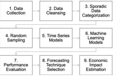
Fig. 2.Analysis Framework

Data Collection: 187,106 transaction lines encompassing spare parts de-mand from 2017 thru 2019, with 28,344 materials of which 24,068 are MTO and the remaining are made-to-stock MTS. In order to improve forecast accuracy additional 20 years of sales history (910,387 + 179,024 transaction lines from legacy ERP systems). For forecast validation purposes we updated our dataset with 2020 data (January thru March) (16,398 records).

Data Cleansing:For purposes of running time series and Croston models we had to summarize the transactional data into monthly buckets including all those periods with zero demand given the high sparsity of some materials. Since demand can only be positive, we filtered out all negative (e.g. returns) transac-tions. In order to avoid unit of measure difficulties, we selected only materials transacted in pieces (i.e. integers). Furthermore, in order to work with reasonable forecastable materials only materials with at least 4 months of positive demand were considered for the following step (Step 3. Sporadic Data Categorization).

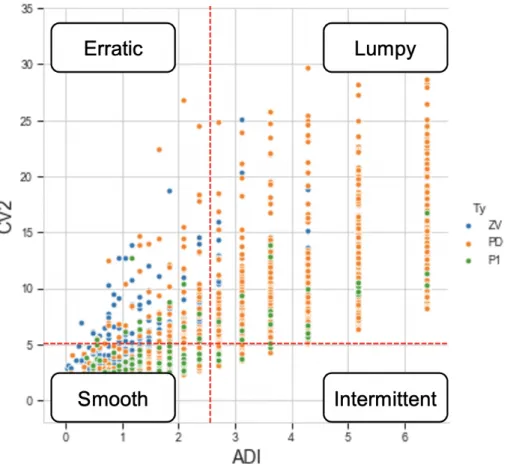
Sporadic Data Categorization: In the literature [17] sporadic demand data were categorized into four types: erratic, lumpy, smooth, and intermittent. For that purpose, we determine Average Demand Interval (ADI) and Coefficient Variance Square (CV2) of the usage volume are adopted as parameters to de-scribe usage patterns [17].

ADI is defined as the average number of time periods between two successive demands which indicates the intermittence of demand. The CV2 is defined as the squared of the ratio of the standard deviation of the demand data divided by the average demand which indicates the variability of demand [17]. (See Fig. 3 in page 4).

Fig. 3.Sporadic Data Categorization [2]

Random Sampling:Proportional to size random sample of parts for each group in Sporadic Data Categorization step.

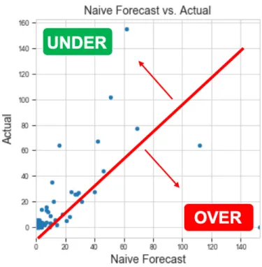
Time Series Models: As suggested by Teunter [12], we introduce two baseline forecasting techniques which are benchmark techniques against with all others are compared. Na¨ıve Forecasting is simply the historical average de-mand (2017-2019), while the Zero Forecast Method produces a prediction of

zero for each month. Those baselines models will be compared against more advanced techniques such as, ARIMA, Croston, improved Croston (TSB), Face-book Prophet.

Machine Learning Models: Random Forest, Artificial Neural Networks (Keras RNN), Extreme Gradient Boosting (XGBoost).

Performance Evaluation:Each forecasting technique has produced 3 pre-dictions (Jan-2020 through March-2020). Each prediction was compared against actual demand and summarized using the Forecast Economic Gain function.

Forecasting Technique Selection:Based upon step (7) Performance Eval-uation and practical considerations we select the forecasting technique which maximizes the Forecast Economic Gain.

Economic Impact Estimation:Leveraging the Forecast Economic Gain function we summarize the net economic gains of the selected forecasting tech-nique for each material in the sample.

2.2 Data Collection

The data that is used in this study is from an Original Equipment Manufac-turer OEM (as specified in Introduction) having annual sales of approximately USD150 million and specifically the spare parts business representing between $42 and $47 million a year delivered by 4,500 to 6,000 monthly order lines. The company has more than 28 thousand materials (also referred as parts or items or stock keeping units SKU’s). As seen in Figure 5, the vast majority of materials (24,068 out of 28,344 materials) belong to the MTO category (MTO = PD). The second largest category is MTS with 2,226 materials (ZV = 1,951 + P1 = 265).

For forecasting purposes we have collected over almost 1.3 million transac-tion lines representing 3 years of order and shipping informatransac-tion (from 2017 thru 2019). This original dataset has been enhanced with additional product infor-mation, such as, costing and inventory planning parameters. (e.g. MRP Type, Procurement: Purchased vs. Manufactured).

2.3 Data Cleansing

For purposes of running time series and Croston models we had to summarize the transactional data into monthly buckets including all those periods with zero demand given the high sparsity of some materials. Since demand can only be positive, we filtered out all negative (e.g. returns) transactions. In order to avoid unit of measure difficulties, we selected only materials transacted in pieces (i.e. integers). Furthermore, in order to work with reasonable forecastable materials only materials with at least 4 months of positive demand were considered for the following step (Sporadic Data Categorization).

2.4 Sporadic Data Categorization

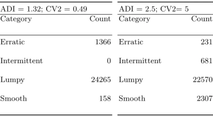
Table 1.Industry recommended vs Adjusted ADI = 1.32; CV2 = 0.49 Category Count Erratic 1366 Intermittent 0 Lumpy 24265 Smooth 158 ADI = 2.5; CV2= 5 Category Count Erratic 231 Intermittent 681 Lumpy 22570 Smooth 2307

As described in [17], it’s recommended to use ADI = 1.32 and CV2 = 0.49 as cutoff values, however using these recommended values categorizes 94% of our materials as lumpy and 0% intermittent, which is impractical for our sampling purposes.

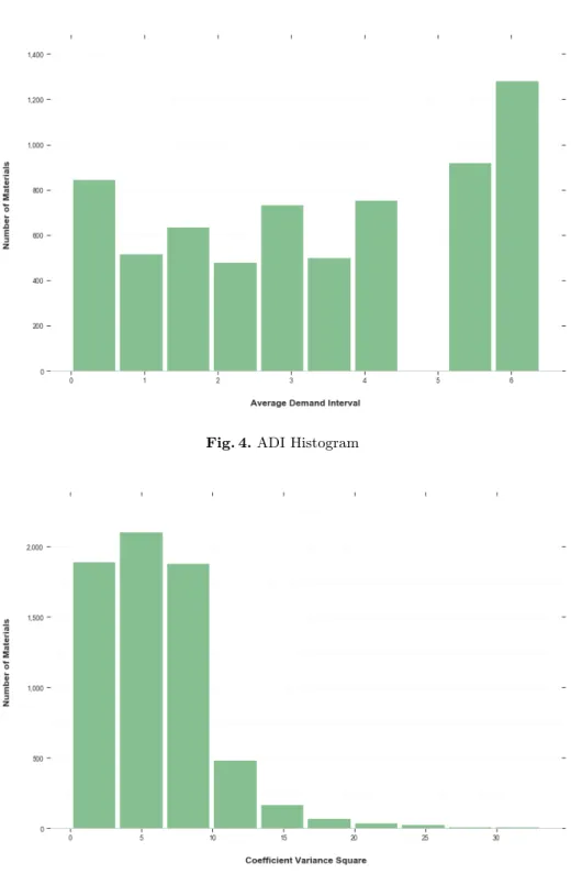
Considering the more sporadic nature of the demand from our dataset made visual in the histograms of ADI and CV2 (Figures 4 & 5 respectively), we made the educated decision of adjusting the cutoff values to: ADI = 2.5; CV2=5. See Table 1 in page 6 for comparison.

By performing a stricter material classification, we have identified Smooth mate-rial in the MTO Type, which represents an opportunity for forecasting. Similarly, all non-Smooth materials (664) in the MTS category represent an obsolescence risk due to their demand patterns as seen in Figure 6.

Table 2.Demand Categorization by MRP Type Category MTO MTS

Erratic 111 120 Intermittent 579 102 Lumpy 22128 442 Smooth 774 1533

Fig. 4.ADI Histogram

2.5 Random Sampling

Due to limited computational resources, we decided to take run an experi-ment with 100 materials. The random sampling technique utilized was propor-tionate stratified sampling, which is a probability sampling method in which different strata in a population are identified and in which the number of el-ements drawn from each stratum is proportionate to the relative number of elements in each stratum1_{. The sampling plan produced utilizing this technique} is displayed in Table 3 in page 9.

Table 3.Sampling Plan Category Count Erratic 3 Intermittent 10

Lumpy 54

Smooth 33

2.6 Time Series Models

Exponential Smoothing: This is a time series forecasting method for uni variate data that can be extended to support data with a systematic trend or seasonal component.These models use a weighted average of past values, in which the weights decline geometrically over time to suppress short-term fluctuations in the data [15]

Ft+1=Ft+α(At−Ft)

Exponential Smoothing2_{can be summarized as an approach that weights recent} history more heavily than distant history.

There are three types of Exponential Smoothing.

– Single Exponential Smoothing : This method is also called asSimple Expo-nential Smoothing. This is a time series forecasting method for uni variate

1

https://www.oxfordreference.com/view/10.1093/oi/authority.20110803100349910 2 _{Exponential Smoothing for Time Series Forecasting}

https://machinelearningmastery.com/exponential-smoothing-for-time-series-forecasting-in-python/

data without a trend or seasonality. It requires a single parameter, called alpha (a), also called the smoothing factor or smoothing coefficient. This parameter controls the rate at which the influence of the observations at prior time steps decay exponentially. Alpha is often set to a value between 0 and 1. Large values mean that the model pays attention mainly to the most recent past observations, whereas smaller values mean more of the history is taken into account when making a prediction.

– Double Exponential Smoothing : This type of exponential smoothing adds support for trends in the uni variate time series. In addition to the alpha pa-rameter for controlling smoothing factor for the level, an additional smooth-ing factor is added to control the decay of the influence of the change in trend calledbeta (b). This method supports trends that change in different ways: an additive and a multiplicative, depending on whether the trend is linear or exponential respectively.

– Triple Exponential Smoothing : This type is extension of Exponential Smooth-ing that explicitly adds support for seasonality to the uni variate time series. In addition to the alpha and beta smoothing factors, a new parameter called gamma (g)is added that controls the influence on the seasonal component. Similar to the trend, the seasonality may be modeled as either an additive or multiplicative process for a linear or exponential change in the seasonality. ARIMA: This is one of the popular and widely used statistical method for time series forecasting. ARIMA is an acronym that stands for AutoRegressive Inte-grated Moving Average. The AR part of the model indicates the regression on the past values of the variable of interest.The MA part indicates that the regres-sion error is actually a linear combination of error terms whose values occurred contemporaneously and at various times in the past. The I (”integrated”) indi-cates that the data values have been replaced with the difference between their values and the previous values.This difference may have been applied more than once. ARIMA 3 can capture complex relationships as it takes error terms and observations of lagged terms. This is a simple stochastic time series model that captures a suite of different standard temporal structures in time series data. The equation for an ARIMA model can be written as

Yt=α+β1Yt−1+β2Yt−2+..+βpYt−pt+φ1t−1+φ2t−2+..+φqt−q

This means that the predicted value for Yt equals Constant + Linear combina-tion Lags of Y (upto p lags) + Linear Combinacombina-tion of Lagged forecast errors (upto q lags). An ARIMA model is one where the time series is differenced at least once to make it stationary and then the AR and the MA terms are com-bined as shown above.

Seasonal ARIMA 4 is another variation of the ARIMA which can be applied

3 _{Understanding Auto Regressive Moving Average Model — ARIMA} https://medium.com/fintechexplained/understanding-auto-regressive-model-arima-4bd463b7a1bb

4

ARIMA Model Time Series Forecasting https://www.machinelearningplus.com/time-series/arima-model-time-series-forecasting-python/

to Time Series data which has a seasonal pattern. In this type of model, Sea-sonal differencing is applied to the Time Series data. ThisSeasonal differencing means subtracting the time series value from the previous season. Seasonality component in any time series problem is subjective. It could be time of day or dailyor weeklyor monthlyor yearly.

ARMA: ARMA stands for “Autoregressive Moving Average” and ARIMA stands for “Autoregressive Integrated Moving Average.” The only difference, then, is the “integrated” part. Integrated refers to the number of times needed to difference a series in order to achieve stationarity, which is required for ARMA models to be valid. Given that the SKUs fall under the 4 different Categorization where intermittent and Lumpy has large variation in Time or interval between two demands and Erratic demand which has regular occurrences in time with high quantity variations. It is difficult to identify the common differencing factor for all 100 materials. Determining an effective differencing factor for each material will be time impractical. Hence ARMA model with lowest AIC score is selected based on the output from aic5.wge function in tswge package.

2.7 Croston Method

Croston Model [15] : For intermittent demand, estimating demand prob-ability (via interval size) and demand size separately was more intuitive and accurate. Let Zt be the estimate of mean non-zero demand size for time t, Vt the estimate of mean interval size between non-zero demands. Xt again denotes actual demand observed at time t, and q is the current number of consecutive zero-demand periods. Yt will denote an estimate of mean demand size (i.e. tak-ing zero demands into the calculation). Then:

Key limitation for Croston model is when there is no demand occurrence, fore-cast does not change

Teunter, Syntetos & Babai (TSB): [13], 5 _{TSB is an improvement to the} Croston model. The idea is to allow the model to update (decrease) its periodicity estimate even if there is no demand observation. That’s perfect as this limitation

5

Croston forecast model for intermittent demand https://medium.com/analytics-vidhya/croston-forecast-model-for-intermittent-demand-360287a17f5f

was the main one we had with the vanilla Croston model.

Level — The TSB model does not change how the level is estimated compared to the regular Croston model.

Periodicity — The periodicity p will now be expressed as the probability to have a demand occurrence. Actually p will now denote a frequency (i.e. a probability) ranging from 0 (demand never occurs) to 1 (demand occurs at every period). We will update this periodicity at every period –even if there is no demand occurrence. The periodicity will decrease if there is no demand occurrence (as you expect a reduction in the probability for a demand to occur). This decrease will be exponential (like for all the exponential smoothing models). The periodicity will increase if there is a demand occurrence.

2.8 AI/ML Platform

Supervised learning6 _{is where you have input variables (x) and an output} variable (Y) and you use an algorithm to learn the mapping function from the input to the output.

Y =f(X)

The goal is to approximate the mapping function so well that when you have new input data (x) that you can predict the output variables (Y) for that data. Artificial Neural Networks (ANN)7_{is a supervised learning system built of} a large number of simple elements, called neurons or perceptrons. Each neuron can make simple decisions, and feeds those decisions to other neurons, organized in interconnected layers. Together, the neural network can emulate almost any function, and answer practically any question, given enough training samples and computing power. A “shallow” neural network has only three layers of neurons: An input layer, that accepts the independent variables or inputs of the model, Hidden layer and An output layer that generates predictions A perceptron is a binary classification algorithm modeled after the functioning of the human brain—it was intended to emulate the neuron. The perceptron, while it has a simple structure, has the ability to learn and solve very complex problems. A multilayer perceptron (MLP) is a group of perceptrons, organized in multiple layers, that can accurately answer complex questions. Each perceptron in the first layer (on the left) sends signals to all the perceptrons in the second layer, and so on. An MLP contains an input layer, at least one hidden layer, and an output layer.

A Deep Neural Network (DNN) has a similar structure, but it has two or more “hidden layers” of neurons that process inputs.Goodfellow, Bengio and Courville showed that while shallow neural networks are able to tackle complex

6

Supervised Machine Learning https://machinelearningmastery.com/supervised-and-unsupervised-machine-learning-algorithms/

7

Neural Network Concepts https://missinglink.ai/guides/neural-network-concepts/complete-guide-artificial-neural-networks/

Fig. 7.Multi Layer Perceptron.

problems, deep learning networks are more accurate, and improve in accuracy as more neuron layers are added. Additional layers are useful up to a limit of 9-10, after which their predictive power starts to decline. Today most neural network models and implementations use a deep network of between 3-10 neuron layers. Recurrent neural networks or RNNs are a family of neural networks for pro-cessing sequential data. Much as a convolutional network is a neural network that is specialized for processing a grid of values such as an image, a recurrent neural network is a neural network that is specialized for processing a sequence of values. Just as convolutional networks can readily scale to images with large width and height, and some convolutional networks can process images of vari-able size, recurrent networks can scale to much longer sequences than would be practical for networks without sequence-based specialization. Most recurrent networks can also process sequences of variable length.

Random forests8or random decision forests are an ensemble learning method for classification, regression and other tasks that operate by constructing a mul-titude of decision trees at training time and outputting the class that is the mode of the classes (classification) or mean prediction (regression) of the individual trees. Random decision forests correct for decision trees’ habit of overfitting to their training set.

Facebook Prophet: As described by Taylor and Letham at Facebook [11], Prophet is a procedure for forecasting time series data based on an additive model where non-linear trends are fit with yearly, weekly, and daily seasonality, plus holiday effects. It works best with time series that have strong seasonal ef-fects and several seasons of historical data. Prophet is robust to missing data and shifts in the trend, and typically handles outliers well9_{. Prophet uses a modular} regression model that often works well with default parameters, and that allows analysts to select the components that are relevant to their forecasting problem

8

Random Forest https://en.wikipedia.org/wiki/Random forest/ 9

and easily make adjustments as needed. The second component is a system for measuring and tracking forecast accuracy, and flagging forecasts that should be checked manually to help analysts make incremental improvements [11].

Light Gradient Boosted Machine with exogenous features(LGBMq)10_: LightGBM, short for Light Gradient Boosted Machine or LGBM, is a library developed at Microsoft that provides an efficient implementation of the gradient boosting algorithm.

The primary benefit of the LightGBM is the changes to the training algorithm that make the process dramatically faster, and in many cases, result in a more effective model LGBM original model was enhanced by adding quotation infor-mation as a leading indicator of future demand.

2.9 Performance Evaluation MAPE:

MAPE is the average of absolute percentage errors(APE). Let At and Ft denote the actual and forecast values at data point t, respectively. Then, MAPE is defined as: M AP E= 1/n n X t=1 |(At−Ft)/At|

where n is the number of data points. MAAPE:[5] M AAP E = 1/n n X t=1 arctan(|A−F/A|) (GMAMAD/A):[17]

Geometric Mean of the Mean Absolute Deviation Average (GMAMAD/A) as a robust performance measure. For each series the mean absolute deviations (MAD) is calculated and divided by the mean of the corresponding series RMSE:[14]

Root Mean Square Error (RMSE) is not scaled to demand,

RM SE=

q

1/nXe2

t

whereet=ft−dt, ft=forecast or prediction,dt= actual demand, n = number

of historical periods with actual demand and a forecast Root Mean Squared Logarithmic Error(RMSLE):11 10 https://machinelearningmastery.com/gradient-boosting-with-scikit-learn-xgboost-lightgbm-and-catboost/ 11 https://scikit-learn.org/stable/modules/model evaluation.htmlmean-squared-log-error

The mean squared logarithmic error function computes a risk metric corre-sponding to the expected value of the squared logarithmic (quadratic) error or loss.

If ˆyi is the predicted value of the i-th sample, andyi is the corresponding true

value, then the mean squared logarithmic error (MSLE) estimated over n sam-ples is defined as RM SLE(y,yˆ) = v u u t1/n n−1 X i=1 (ln(1 +yi)−ln(1 + ˆyi))2

This metric is best to use when targets having exponential growth, such as pop-ulation counts, average sales of a commodity over a span of years etc. Note that this metric penalizes an under-predicted estimate greater than an over-predicted estimate.

Forecast Economic Gain function:

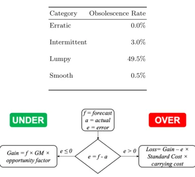
As stated earlier, inventory management focuses on balancing the cost of holding the items in inventory and the penalty of running out. Existing forecast accuracy measurements are unbiased, meaning they penalize over forecasting (i.e. prediction greater than actual) and under forecasting (i.e. prediction less than actual) equally. In a realistic supply chain context the consequences of over or under forecasting may have very different financial impact. For that reason we propose a new measurements which balances the gains of a good prediction (i.e. lead time reduction for instance) versus the negative consequences of over forecasting (e.g. procuring more stock than necessary, which will lead to future obsolescence disposition costs) [16]. The Forecast Economic Gain function is measured in USD dollars, therefore it’s comparable across different dimensions and additive - both clear advantages over other forecast error measurements, which are material specific. On the plus side (gains), we assume a 12.5% in-crease in volume thanks to lead time reduction leading to a higher capture (i.e. quotation win) rate. On the negative side (loss), in this specific business context we must account for obsolescence risk [4]. The probability of not being able to move stock in the future is not the same across the board. By analyzing year-over-year demand behavior, we were able to assess the probability of no demand for next year (we used 2019 for our analysis). Not surprisingly, as displayed in Table 4 in page 16, the probability of experiencing no demand for a full year is close to 50% for the lumpy category. On the opposite side of the spectrum, smooth materials (a lot more predictable) have a very low chance of experiencing no demand i.e. obsolescence rate.

Previous analysis has demonstrated that a lead time reduction equivalent to 90 days can increase the win rate (on quoted business opportunities) by 12.5%. Therefore, one of the assumptions incorporated into the Forecast Economic Gain function is that an accurate forecast reduces the procurement lead time by 90 days increasing the chance of higher sales by a factor of 0.125.

Table 4.Obsolescence Rate Category Obsolescence Rate

Erratic 0.0%

Intermittent 3.0%

Lumpy 49.5%

Smooth 0.5%

Fig. 8.Forecast Economic Gain Function

3

Final Results

3.1 Forecasting Technique comparison using monthly data with random sampling:

Initial comparison of different techniques was performed using monthly data with random sampling of 100 units (SKUs). Based on the maximum Forecast Economic Gain function (FEGf), the selections are (in descending order, from most to popular to least) displayed in Table 5.

The baseline models (Na¨ıve and Zero) outperform all the Time Series and ML models accounting for 64% of the selections (36% and 28% respectively). The second tier is composed by the most promising ML models XGB and Ran-dom Forest (7% each).

The third tier includes the Time Series Models: FB Prophet, Croston and ARIMA. Keras outperformed other techniques for only 2 materials.

Analyzing the selection by category, we see that in the largest category -and most difficult to forecast, Lumpy with 54 materials, the baseline models (Na¨ıve and Zero) are the uncontested winners with 40 selections.

The second most populous category and easiest to forecast, Smooth with 33 ma-terials, the selection is evenly distributed across the board, but Na¨ıve is still the

Table 5.Forecasting Technique Selection (monthly data & n=100) Technique % FEGf Na¨ıve 36% $2,195 Zero 28% $0 XGB 7% $1,299 Random Forest 7% $1,331 FB Prophet 6% $7 Croston 6% $1,752 ARIMA 5% $574 Croston TSB 3% $2,010 Keras 2% $1,014

most popular.

Fig 9 demonstrates how balanced the Na¨ıve Forecasting behaves across 100 ma-terials. On the other hand, Fig 10 shows the high price Keras had to pay for a few materials where it over forecasted heavily.

The summation of the Forecasting Economic Gain function (FEGf) across all 100 materials in the sample per technique (see Table 5) gives us the chance to look at how a forecasting technique performed across all materials and whether the gain of its predictions outweighs the cost (obsolescence due to over forecast-ing).

In accordance to the Forecasting Technique selection percentage, the Na¨ıve base-line method outperforms all other methods. On the other hand, the Zero tech-nique produces zero gains and zero costs by definition.

In contrast to the forecasting technique selection percentage, where Croston TSB was the favorite technique of only 3% of the materials, it produces the second largest gain.

Other Time Series models, FB Prophet and ARIMA, under perform under this dimension.

3.2 Forecasting Technique Selection Comparison Quarterly Data: Final comparison of techniques was done against quarterly data on all materi-als (6415 SKUs). During this analysis, we have leveraged a strategy of training a single model to forecast multiple time series at the same time. Based on combined metrics of Economic Gain Function and RMSLE, the selections are displayed in Table 6.

The LGBM model with exogenous data from quotation information (LGBMq) outperform in all the categories. For smooth category, FB Prophet is performing equally with LGBMq model.

Table 6 gives us the indication on how the techniques performed across all categories based on the Forecasting Economic Gain function, RMSLE and pro-cessing time.

4

Ethics

In our particular case, the only ethical concern was to safeguard customer data and financial information related to the OEM who kindly shared detailed transactions for our study. Having said that, our first line of defense was to main-tain the anonymity of the data provider and ensure it could not be inferred from the datasets utilized. Secondly, due to the sensitivity of the financial informa-tion (i.e. product margins and discounts), customer names were removed from the datasets. Last but not least, data aggregation (monthly and/or quarterly) provides the last line of defense for data privacy and confidentiality.

Table 6.Forecasting Technique Comparison (quarterly data & n=6415) Technique Economic Gain RMSLE Time (in seconds)

Zero $0 1.75 0 Na¨ıve $154,293 1.22 0 Croston $154,409 1.09 239 FB Prophet $210,396 1.14 10,709 Random Forest ($184,219) 1.26 2,434 LGBM $109,324 0.94 33 LGBMq (exogenous) $161,873 0.87 12

5

Conclusions

Similar to what we found in researched literature [9][17][6], machine learn-ing models tend to outperform time series techniques produclearn-ing more accurate predictions closer to the actual data (See Table 5). In our experiment, with 100 sample materials encompassing all 4 different demand patterns, XGB and RF indeed outperform ARIMA. However, when comparing the overall performance against baseline methods (Na¨ıve and Zero), we found that baseline methods ac-tually outperform sophisticated time series models (FB Prophet and ARIMA) and even machine learning models (XGB, RF, Keras RNN). Therefore, based on the overall Forecast Economic Gain, forecasting -as described in this paper- is not a financially attractive option to the business. Our experiment shows that aggregating the demand in quarterly buckets and training single model for fore-casting all the materials yields superior results, especially enhancing demand history with quotation activity as exogenous data in all the 4 categories. As future improvement opportunity, as suggested by Petropulos [7], we propose to consider ensemble (i.e. forecast combinations) and exogenous methods, which consider quotation activity and/or the installed base [1].

References

1. Van der Auweraer, Sarah, B.R.S.A.: Forecasting spare part demand with installed base information: a review. International Journal of Forecasting (2017)

2. Chen, Jing, e.a.: Maintenance, repair, and operations parts inventory management in the era of industry 4.0. International Federation of Automatic Control (2019) 3. Croston, J.D.: Forecasting and stock control for intermittent demands. Operational

Research Quarterly (1970-1977)23, No. 3, 289–303 (1972)

4. Jaarsveld, Willem van, D.R.: Estimating obsolescence risk from demand data - a case study. Report Econometric Institute EI (2010)

5. Kim, Sungil, K.H.: A new metric of absolute percentage error for intermittent demand forecasts. International Institute of Forecasters (2016)

6. Nemati, A, B.A.S.M.T.R.: Demand forecasting for irregular demands in business aircraft spare parts supply chains by using artificial intelligence (ai). International Federation of Automatic Control (2017)

7. Petropoulos, Fotios, K.N.: Forecast combinations for intermittent demand. Journal of the Operational Research Society (2015)

8. Shahrabi, e.a.: Supply chain demand forecasting; a comparison of machine learning techniques and traditional methods. Journal of Applied Sciences (2009)

9. Shahrabi, J, M.S.H.M.: Supply chain demand forecasting; a comparison of ma-chine learning techniques and traditional methods. Asian Network for Scientific Information (2009)

10. Singh, S.R., K.T.: Forecasting aviation spare parts demand using croston based methods and artificial neural networks. Journal of Economic and Social Research (2011)

11. Taylor, Sean, L.B.: Forecasting at scale. Facebook (2017)

12. Teunter, RH, D.L.: Forecasting intermittent demand: a comparative study. Oper-ational Research Society Ltd (2009)

13. Teunter, Ruud, S.A.B.Z.: Intermittent demand: Linking forecasting to inventory obsolescence. European Journal of Operational Research (2011)

14. Vandeput, N.: Data science for supply chain forecast, 1st edition (2018) 15. Waller, D.: Methods for intermittent demand forecasting

16. Zied Babai, Mohamed, S.A., Teunter, R.: Intermittent demand forecasting: An empirical study on accuracy and the risk of obsolescence. International Journal of Production Economics (2014)

17. S¸ahin, Merve, K.R.D.: Forecasting aviation spare parts demand using croston based methods and artificial neural networks. Journal of Economic and Social Research (2013)