Configuration of Deep Neural Networks Using Model-Based Optimization

(1)

Ludwig-Maximilian University of Munich

Master Thesis

Configuration of Deep Neural Networks

Using Model-Based Optimization

A thesis submitted in fulfillment of the requirements for the degree of

Master of Science in Statistics at the

Department of Statistics

Author: Benjamin Klepper

Supervisor 1: Prof. Dr. Bernd Bischl

Supervisor 2: Janek Thomas

Study program: Statistics with Focus on Economics and Social Science

January 3, 2018

(2)

(3)

Declaration of Authorship

I, Benjamin Klepper, declare that this thesis titled “Configuration of Deep Neural Networks Using Model-Based Optimization” and the work presented in it are my own. I confirm that: • This work was done wholly or mainly while in candidature for a research degree at

this University.

• Where any part of this thesis has previously been submitted for a degree or any other qualification at this University or any other institution, this has been clearly stated. • Where I have consulted the published work of others, this is always clearly attributed. • Where I have quoted from the work of others, the source is always given. With the

exception of such quotations, this thesis is entirely my own work. • I have acknowledged all main sources of help.

Date: Signed:

(4)

(5)

Abstract

Deep neural networks have improved the performance results in image recognition, speech recognition and many other domains. Manually configuring the architecture and other hyperparameters of deep neural networks becomes unfeasible for large hyperparameter spaces. Automating this process requires the optimization of an expensive black-box func-tion over a mixed and hierarchical search space. Model-based optimizafunc-tion is a state-of-the-art derivative-free technique for optimizing expensive black-box functions. This thesis extends the standard model-based optimization approach to take into account the high computational costs and search space complexity when configuring deep neural networks. The resulting algorithm’s performance is compared to random search, the standard model-based optimization approach and a hand-designed model on CIFAR-10, Fashion-MNIST

and MNIST rotated with background image. For this purpose, the R machine learning

packagemlr is extended to include functionalities of the deep learning framework MXNet. Of all algorithms, the standard model-based approach achieves the best average rank across all data sets. Nevertheless, all algorithms yield comparable results. On average, the hand-designed model outperforms the automatically configured models. The results indicate that the automatic configuration of kernel and stride sizes for convolutional layers of neu-ral networks is inefficient when choosing the values independently. Seveneu-ral possibilities for improving the performance of the model-based optimization extension are proposed.

(6)

(7)

List of Figures

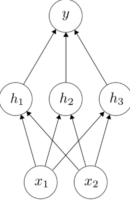
2.1 A multilayer perceptron with one hidden layer. . . 11

2.2 Example of a convolution. . . 13

3.1 Example of sequential model-based optimization. . . 21

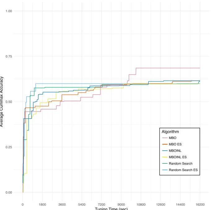
5.1 Tuning runs on CIFAR-10. . . 49

5.2 Average performance on CIFAR-10. . . 50

5.3 Examples of number and type of layer configurations on CIFAR-10. . . 51

5.4 Tuning runs on Fashion-MNIST. . . 52

5.5 Average performance on Fashion-MNIST. . . 53

5.6 Tuning runs on MNIST rotated with background image. . . 54

5.7 Average performance on MNIST rotated with background image. . . 55

5.8 Convolutional configurations of MBO and MBOINL. . . 56

5.9 Performance rank of the algorithms. . . 57

(10)

(11)

List of Acronyms

AI artificial intelligence

CIFAR Canadian Institute for Advanced Research

DACE Design and Analysis of Computer Experiments

EGO Efficient Global Optimization

EI expected improvement

GP Gaussian process

MBO model-based optimization

MBOINL model-based optimization with increasing number of layers

PI probability of improvement

ReLU rectified linear unit

RF random forest

SGD stochastic gradient descent

(12)

(13)

Chapter 1 Introduction

People speculated about programmable computers becoming intelligent when they were first conceived, which was over a hundred years before one was actually built [1]. Cur-rently, artificial intelligence (AI) is a very active, rapidly growing area of research with a wide range of practical applications like speech recognition [2], image recognition [3], ma-chine translation [4], automating repetitive tasks and making medical diagnoses [1]. In its early days, AI was used very successfully to solve problems that are intellectually difficult for humans and which can be formalized by a set of mathematical rules [1]. More challeng-ing, however, are problems that humans solve intuitively but that are hard to formalize, like recognizing objects [1].

Several projects employing a knowledge-based approach to artificial intelligence (attempt-ing to hard-code knowledge in a formal language) have not led to a major success [1]. This suggests that AI algorithms should be given the ability to extract their own knowledge from data [1].

Machine Learning models are models that can acquire knowledge by extracting patterns from raw data. These models can be used to identify objects in images, make product rec-ommendations based on user preferences and select relevant results for web search queries. They are therefore present in many services and products, for example in e-commerce, social networks and also increasingly in cameras and smartphones [5].

While simple machine learning algorithms can help make decisions of a seemingly subjec-tive nature like recommending cesarean delivery or detecting spam email, their performance depends on the representation of the provided data. Ideally, this data would consist of fea-tures that are highly correlated with the output. In contrast, providing pixels of an image for object detection would probably result in poor performance when using simple machine learning algorithms.

As the ability of simple machine learning models to process raw data is limited, profound domain knowledge and careful engineering is required to design and extract features from the original raw data and transform them into a suitable representation to serve as input for the machine learning model. Many learning tasks can be solved by designing and ex-tracting meaningful features from data and applying a simple machine learning algorithm to them [1].

(14)

Prior to deep learning methods, many applications of machine learning combined hand engineered features with linear classifiers, which can only divide the input space into half-spaces separated by a hyperplane [5]. Complex problems like image recognition require the model to be insensitive to irrelevant variations of the input, like the position of an object, but sensitive to relevant variations like the difference between a white wolf and a white wolf-like dog [5]. On a pixel level, a linear classifier would be very sensitive to the former but rather insensitive to the latter and would therefore require pre-designed features. Designing features may prove to be a difficult endeavour. In image recognition it can be difficult to describe a certain object in terms of pixel values as for example angle, position and brightness can vary for different images.

Representation learning refers to methods that can discover suitable representations from the data automatically [5]. In representation learning, machine learning is not only used to construct a mapping from the features to the output but also from the input data to the features (representation). Algorithms equipped with this capability can easily be applied to different kinds of tasks with little manual overhead while yielding very good performance, often better than with manually designed features [5].

Good features should separate the factors of variation in the data, which may be unob-served directly in the data but affect the obunob-served data [1]. These factors can also be concepts or abstractions and can once again be illustrated with the angle, position and brightness of an object in a picture. Depending on the level of abstraction, some factors of variation may be difficult to extract directly from the data.

Deep learning solves this problem by employing a hierarchical approach to learning repre-sentations so that more abstract reprerepre-sentations can be learned from previously learned, simpler representations. Deep learning models are therefore representation learning models with a hierarchy of representational levels and hence several levels of abstraction [5]. This hierarchical concept of representations that build upon each other and become increas-ingly complex allows the computer to learn more complicated concepts. The models are composed of multiple processing layers, each layer often a simple but non-linear module that transforms the representation to a more abstract one. Each layer has certain internal parameters to compute the representation of the data using the previous layer’s represen-tation [5]. An algorithm might first learn to detect different kinds of edges, then to detect shapes using combinations of edges and then to detect objects as combinations of shapes. A graph of the hierarchy of representations is multilayered and deep, hence the name deep learning.

An alternative interpretation of deep learning is that it is a sequential computer program with each layer being the state of the memory after executing a set of instructions in paral-lel. As an instruction in a sequence of instructions can refer to previous ones, the sequential approach offers greater flexibility. The difference in this kind of interpretation is that not all of the parameters in the model encode factors of variation but also state information to help execute the program that in turn produces a meaningful output from the input [1]. In recent years, deep learning has beaten other machine learning techniques not only at image recognition [6, 7] and speech recognition [8, 9] but also other tasks like reconstructing brain circuits [10], natural language understanding [11] and analyzing particle accelerator

(15)

3 data [12].

The applications in practice thus increasingly make use of deep learning methods. When a sufficient number of transformations are composed, complex structures can be learned from data. In image classification, the first layer may represent edges (and whether they are present or absent) at certain locations. The second layer may detect specific arrangements of edges. The third layer may combine these arrangements to parts or objects. There-fore, the higher layers of representation are influenced less by unimportant variation in the data. The representation learned at each layer is extracted from the data without human supervision by using a general learning approach.

Supervised learning is the most common form of machine learning [5]. In supervised learn-ing, the data used for training the model contains a so-called target, giving the correct output value for the feature values associated with it. Using an objective function that measures the error for the correct output and the output values computed by the model, the model adjusts its internal parameters to reduce the error. This objective function is also called performance measure.

In a deep learning model these internal parameters, also called weights, occur in large numbers. To correctly modify the weights, the learning algorithm typically computes the gradient vector which indicates how the error would change if the weights changed by a small amount. The weights are then adjusted in the opposite direction of the gradient (as the gradient gives the direction of the steepest ascent and the error should be minimized). A very commonly used method is stochastic gradient descent (SGD) [5], which consists of repeatedly updating the weights with the average gradient of a random subsample of the training data. The gradient of each sample is a noisy estimate of the average gradient of the complete training data. After training, the performance of the model is measured on a different data set called test set. This provides a more reliable estimation of the model’s ability to generalize (make meaningful predictions for unseen inputs).

Like the majority of machine learning algorithms, neural networks have so-called hyper-parameters, parameters whose values are not learned during training and therefore have to be set in advance. The process of selecting a good (in some meaningful way) setting of hyperparameters is also referred to as tuning. In many cases, tuning the hyperparameters of neural networks proves to be especially difficult for several reasons.

First, neural networks may be sensitive to the hyperparameter setting, therefore it must be chosen carefully.

Second, the tuning process includes optimizing discrete and conditional hyperparameters, especially when configuring the architecture of a neural network. Additionally, the number of tunable hyperparameters can be very high compared to other machine learning mod-els. The resulting hyperparameter space is a high-dimensional and non-trivial hierarchical search space.

Third, training a neural network can be computationally very costly. Designing neural net-works by hand therefore requires expert knowledge and is in many cases not feasible [13]. Naturally, choosing good hyperparameters automatically with an efficient optimization al-gorithm is very desirable.

(16)

Optimization is a field of study that a great deal of research has been devoted to and that finds application in a wide range of areas, e. g., economics or mechanical design [14]. One specific problem setting is the optimiziation of a nonlinear function (the so-called objective function) over a compact set. Common assumptions include that this objective function has a closed analytical form which is known or is cheap to evaluate [15]. In prac-tice, however, the objective function is often a black-box function [15]. These functions can be viewed as systems that produce numeric output given some input without much knowledge about their inner workings being available, also resulting in an unavailability of gradients [16]. Additionally, they may be expensive to evaluate as they often correspond to expensive processes like drug trials or financial investments [15]. Black-box functions also occur for many problems in machine learning, for example when optimizing hyper-parameters of machine learning algorithms (see, e. g., [17, 18, 19]). In this scenario, the inputs of the black-box function could be the hyperparameters of the algorithm and the output one or more performance measures. More complex scenarios are also possible, e. g. optimizing a machine learning pipeline (see [16]). Optimizing a black-box function entails being restricted to obtaining observations by evaluating the function at sampled values and receiving a possibly noisy response. Since evaluations are expensive, it is desirable to optimize the function using a minimal number of evaluations. Due to the function’s nature, optimization techniques that require differentiability or independent parameters are not directly applicable.

A lot of research has been devoted to finding good hyperparameters automatically using various approaches like random search [20], bandit-based approaches [21] and model-based optimization (MBO) (also called Bayesian optimization) [22, 23].

Other possible techniques are, for example, evolutionary algorithms [24, 25] and reinforce-ment learning [26, 27, 28]. However, both of these methods either have high demand for computational resources or are not competitive regarding their performance [13, 29]. MBO is a derivative-free approach for global optimization of black-box functions. Incor-porating a sequential design strategy when applying MBO, also called sequential model-based optimization (SMBO) [30], has become an optimization strategy with state-of-the-art performance [16]. In MBO, the objective function (e. g. the machine learning model’s performance) is approximated using a statistical model (e. g. a Gaussian process (GP)). This so-called surrogate model is then used to propose a new point that is likely to yield good performance according to some pre-defined criterion. Applying the standard MBO approach to tuning neural networks has revealed several areas with potential for improve-ment.

First, only numerical parameters can be tuned with a Gaussian process surrogate model when using a standard kernel. Hutter and Osborne [31] define a kernel for mixed continu-ous and discrete parameter spaces. Building on this, Swersky et al. [32] introduce kernels for Bayesian optimization of conditional parameter spaces. Wang et al. [33] introduce a new technique to eliminate the need for optimizing the acquisition function. L´evesque et al. [34] use model-based optimization for conditional hyperparameter spaces by injecting knowledge about conditions in the kernel. This is illustrated by simultaneously doing

(17)

al-5 gorithm selection and hyperparameter tuning.

Second, the scalability of MBO to higher dimensional parameter spaces can be improved. Wang et al. [35] use random embeddings to improve the scalability of Bayesian optimization to high dimensions for domains of continuous as well as discrete variables. Springenberg et al. [36] introduce an approach of using neural networks as surrogate models to improve the scaling of Bayesian optimization regarding the number of both hyperparameters and evaluations of the objective function.

Third, since training neural networks may become computationally costly, it is desirable to improve the resource allocation in the MBO process. Yogatama and Mann [37] propose a method of MBO that aims to reduce computational time by transferring information between data sets using a common response surface. Klein et al. [37] introduce a Bayesian optimization procedure which models loss and training time with respect to the size of the training set to extrapolate the validation error for a subsample of the training set to the whole training set. Feurer et al. [38] explore a way of transferring knowledge of hyper-parameter configurations between data sets by using a metalearning procedure to propose the initialization of the MBO tuning process. Swersky et al. [39] provide a new technique for Bayesian optimization to decide when the training process of a model should be paused to start with a new one or continue training a previously paused one. This is done for models that are trained in an iterative fashion including neural networks. Illievski et al. [40] introduce a way to make Bayesian optimization for tuning deep neural networks more efficient by using a deterministic surrogate model. Smithson et al. [41] propose tuning neural networks by using Bayesian optimization with multi-objective exploration of the hyperparameter space using a neural network as the surrogate model, aiming to reduce the number of objective function evaluations. Domhan et al. [42] introduce a technique to extrapolate the learning curves of neural networks during training, aiming to determine if the training process should be stopped early to improve resource allocation. Hutter et al. [43] propose an MBO algorithm that can handle categorical parameters by using a random forest based surrogate model. Elsken et al. [13] use network morphisms (introduced as network transformations by Chen et al. [44]) to generate pre-trained models in optimizing the architecture of convolutional neural networks to reduce computational costs. Liu et al. [29] propose configuring the architecture of convolutional neural networks by training architectures with increasing complexity using a SMBO approach with a recurrent neural network surrogate and no acquisition function, matching state-of-the-art performance. Besides these main points, other approaches to extend the MBO framework have been proposed. For example, Wu et al. [45] introduce a new Bayesian optimization algorithm that uses derivative information.

Welchowski and Schmid [46] tune kernel deep stacking networks using a combination of MBO and hill climbing.

This thesis presents an approach to extend MBO for tuning the hyperparameters (in-cluding the architecture) of feedforward and convolutional neural networks by combining MBO with a procedure inspired by hill climbing and multi-fidelity optimization. The new approach is compared to random search and the standard MBO method on CIFAR-10 [47],

(18)

Fashion-MNIST [48] and MNIST rotated with background images (used in [20], a varia-tion of the well-known MNIST data set [49]). To carry out these benchmarks, a dedicated extension of the popular R [50] machine learning package mlr [51] is created to integrate functionalities of the MXNet [52] deep learning framework. All MBO procedures are done using the R package mlrMBO[16].

The remainder of the thesis is structured as follows: The concept of feedforward neural networks is introduced, focusing on fully connected and convolutional layers. Then, an overview of MBO is given and the model-based optimization with increasing number of

layers (MBOINL) algorithm is introduced. Subsequently, the software, namely mlr,

ml-rMBO and MXNet, is described and illustrated by some examples. Finally, benchmark

results are presented, followed by the summary and conclusion. All figures regarding the benchmark results have been created with R using the batchtools [53] package, the figures on neural networks and MBO have been created with Inkscape [54].

(19)

Chapter 2 Deep Neural Networks

2.1 History of Deep Learning

While the field of deep learning received its name fairly recently, its roots are in the 1940s. There have been three main waves of development.

In the 1940s-1960s the first wave was known as cybernetics, where simple linear models were used with a neuroscientific motivation (see, e. g., [55]). The limitations of linear mod-els led to a decline of interest in neuroscientifically inspired learning, causing the first dip in popularity.

The second wave was from the 1980s to the mid-1990s and emerged from connectionism,

which arose in the context of an interdisciplinary study of the mind called cognitive sci-ence, with the central idea that simple computational units achieve intelligence by being connected in a network [1]. A key concept from connectionism isdistributed representation (see [1]): Each input in the representation should be represented by multiple features and each feature should be relevant for the representation of multiple inputs. Suppose the input is an image of either a cat or a dog, which is either brown or black. A possible representation of the input is to have a binary feature for each possible input, resulting in four features (featuresblack cat, black dog,brown cat and brown dog, where exactly one has value 1 and the others have values 0). A distributed representation would be to have a feature for the type of animal (cat or dog) and for the color (brown or black).

Several groups independently discovered a simple way to train multilayer networks during the 1970s and 1980s using SGD [56] [57, 58, 59]: As long as the individual modules from the multilayer stack can be represented by sufficiently smooth functions of inputs and internal weights, the gradients can be obtained by using the so-called backpropagation procedure. The backpropagation procedure is basically an application of the chain rule for derivatives to compute the gradient of the objective function with respect to the internal weights of the multilayer network (by working backwards through the network from layer to layer). Arguably, the work of Rumelhart et al. [59] had the most impact [1]. The second wave of neural networks ended because unfulfilled expectations driven by unrealistic claims of AI ventures coincided with other AI approaches achieving good results [1].

(20)

In the late 1990s neural networks were in large parts ignored by the communities of ma-chine learning, computer vision and speech recognition since the approach was considered infeasible due to the risk of the gradient descent stopping in local minima [5]. Theoretical and empirical results suggest, however, that local minima are rarely a problem. Instead, the search space often contains saddle points where the gradient is zero and more impor-tantly the values of the objective function are very similar. Hence, it does not make a big difference at which saddle point the algorithm is stuck [5].

In 2006 a research collaboration organized by the Canadian Institute for Advanced Re-search (CIFAR) resulted in creating unsupervised learning algorithms (algorithms that learn from data that consists of examples {x} without any corresponding target value) that could create multilayered feature detectors from unlabelled data. A multilayered fea-ture detector would be trained with unlabelled data (also called unsupervised pre-training) and afterwards an output layer would be added, creating a neural network with appropriate initial weight values that could be fine-tuned using backpropagation [5]. The third wave of AI research began in 2006 with a breakthrough in training a so-called deep belief network using a method called greedy layer-wise pretraining [60], which was quickly extended to other types of networks [61, 62].

At the time of writing, the third wave is ongoing and deep learning methods regularly outperform alternative AI methods [1]. However, the focus of the third wave has shifted from unsupvervised learning and generalizing from small datasets to leveraging large la-beled datasets. Accordingly, the focus of this work lies on supervised learning.

Besides new techniques to train deep networks, two factors have played a crucial role in the increasing performance of deep learning methods. One is the increasing availability of appropriate and large datasets for machine learning applications. The other is the availability of computational resources, like faster CPUs, the advent of GPUs and better infrastructure for distributed computing, to run larger models. This has resulted in dra-matically improved predictions and accuracy of recognition as well as an increased variety of successful applications.

2.2 Feedforward Neural Networks

Basic artifical neural networks implement a function y(x;w). The central idea is that the algorithm can learn a relationship between inputs xand targett using provided examples. For a givenx, a trained network should then outputythat is close tot(in some appropriate way). Training a network consists of searching the parameter space of weights for values ofw that produces a function fitting the training data well (and generalizes well to unseen examples). Typically, this so-called performance of the model is measured using some objective function (error function) as a function of w. The training process is therefore a function optimization. Many optimization algorithms not only make use of the objective function but of its gradient (with respect to w) as well. For feedforward networks (see Subsec. 2.2.2), the backpropagation algorithm evaluates the gradient of output y w.r.t. w, and therefore the gradient of the objective function w.r.tw [63].

(21)

2.2 Feedforward Neural Networks 9 The following introduction can be found in [63].

2.2.1 Neuron

Neurons are the most basic building blocks for neural networks. We therefore seek to understand them before moving on to more complex networks. Indeed, a single neuron can be viewed as a very simple supervised neural network.

Assume we have a number I ∈_N of inputs xi and one outputy. In a single neuron, each input is assigned a weight wi. Additionally, there may exist an additional parameter w0 called bias, which can be interpreted as the weight of input x0 = 1. An activity rule is a local rule defining how the activity (output) of a neuron changes. The activity rule of a single neuron has two steps:

• An activation a = w>x, with either w = (w0, w1, ..., wI) and x = (x0, x1, ..., xI) or

w= (w1, ..., wI) and x= (x1, ..., xI). • An activation function f.

A single neuron as a binary classifier could receive a number of input vectors {x(n)_}N n=1 with binary labels {t(n)}N

n=1 and produce an outputy(x;w) between 0 and 1 for each x(n). Note that x(n) _{= (}_x(n) 1 , ..., x (n) I ) orx(n) = (x (n) 0 , x (n) 1 , ..., x (n)

I ). An objective function can be chosen as G(w) = − I X n=1 t(n)ln(y(x(n);w)) + (1−t(n)) ln(1−y(x(n);w)). (2.1)

The activity is then computed as y=f(a). Defining

g(n)_j =−(t(n)_j −y_j(n))x(n)_j , (2.2) we can write gj = ∂G ∂wj = N X n=1 g(n)_j . (2.3)

Therefore the gradient ∂G/∂w can be written as a sum of vectorsg(n)_.

A simple on-line gradient descent training algorithm would be to sequentially put each

observed input example through the network and update the weights w in the opposite

direction of g(n)_{. More precisely, the weights are updated by} ∆wi =η(t−y)x

(n)

i . (2.4)

Here, η is thelearning rate, the length of the step of each update, typically between 0 and 1. Choosing the right learning rate is not a trivial task. A learning rate that is too big might result in the updated weight “jumping” over an optimum. A learning rate that is

(22)

very small however may result in very long computation time during the training phase as the small steps lead to a longer time until convergence.

An alternative to this on-line paradigm would be to use a batch of examples to update the weights. For (x(n)_{, t}(n)_{) (}_n _{= 1}_{, ..., K}₎_{, K} _≤_N_{, the update would be ∆}_w

i =PK_n=1g (n) i . The number of updates times the number of examples in one batch can be larger than the actual number of observations in the training data. In this case, the updating process cycles through the data more than once. Therefore, observations are used multiple times for updates but not necessarily in the batch constellation. One update cycle through the training data is called epoch.

The phenomenon of overfitting occurs when the model fits the training data so well that the generalization ability of the model decreases. A high level interpretation would be that at a certain point during training, random noise in the data is interpreted as signal. As the overall aim is to obtain a model with good generalization, it is desirable to avoid overfitting. An intuitive approach called early stopping (see Subsec. 2.4.2) consists of monitoring a metric (usually some indicator of the ability to generalize) during training and utilizing a stopping criterion (e. g. when generalization worsens) to interrupt the training process. Another approach, called regularization, is to modify the objective function to incorporate a bias against unfavorable solutions w. A thorough overview of regularization for deep learning can be found in [1].

2.2.2 Multilayer Perceptron

A neural network is called afeedforward network if the neurons and their connections form a directed acyclic graph. They consist of a sequence of layers of neurons (where the neurons in each layer are not connected to each other). More precisely, they have an input layer, an output layer and a number of layers in between called hidden layers. They can be seen as a nonlinear parameterized transformation of inputs which can be used for regression as well as classification tasks. A fully connected layer is a layer of neurons where each neuron has all neurons from the previous layer as inputs and its output is in turn input to all the neurons from the subsequent layer. A multilayer perceptron is a feedforward network where all hidden layers are fully connected layers, see for example Fig. 2.1. A regression multilayer perceptron with one hidden layer could have I inputsxi, a hidden layer with

a(1)_j = I X l=1 w(1)_jl xl+θ (1) j , hj =f(1)(a (1) j ), j = 1, ..., nhidden (2.5)

and an output layer with

a(2)_i = nhidden X j=1 w(2)_ij hj +θ (2) i ; yi =f(2)(a (2) i ), i= 1, ..., nout, (2.6)

where nhidden is the number of neurons in the hidden layer, nout is the number of output neurons and f(1) _and _f(2) _{are the activation functions.}

(23)

2.3 Convolutional Neural Networks 11

Figure 2.1: A multilayer perceptron with one hidden layer.

2.3 Convolutional Neural Networks

Convolutional neural networks are a special kind of network for data with grid-like topol-ogy. A very easy example would be 1-D time series data or 2-D image data containing the grey scale pixel values. A more complex example would be 3-D image data, such as actual 3-D images, for example medical CT scans, or 2-D color images with three so-called channels respectively containing the red, green and blue value of a pixel, which could also be viewed as a 2-D grid of vectors. As the name suggests, convolutional neural networks make use of a special linear mathematical operation called convolution. In essence, convo-lutional neural networks are feedforward neural networks that use convolution operations in one of the layers. A simple convolutional network could consist of an input layer, a hidden convolutional layer and an output layer that is fully connected to the outputs of the convolutional layer.

2.3.1 Convolution Operation

The convolution operation can be viewed as an aggregation of (function) valuesx(t) with a weighting functionw(t)

s(t) = Z

x(a)w(t−a) da, (2.7)

denoted by s(t) = (x∗w).

(24)

map. If the domain of x is discrete, the convolution takes the following form: s(t) = ∞ X a=−∞ x(a)w(t−a). (2.8)

In practice, the sum consists of finitely many parts. Convolutions also exist for multiple dimensions. A two-dimensional convolution with discrete domain space, inputI and kernel

K would be S(i, j) =X m X n I(m, n)K(i−m, j−n). (2.9)

2.3.2 Motivation

Convolutions leverage three important ideas: Sparse interactions, parameter sharing and equivariant representations [1].

In contrast to a multilayer perceptron with fully connected layers, a convolutional network employs sparse interactions (also referred to as sparse connectivity or sparse weights) in the sense that the kernel does not take into account all inputs when computing a certain feature map value. For a time series, the kernelw(t) = 1₃₁{−1,0,1}(t) would take the average

of the value at timetand its adjacent values. Therefore, the feature map would simplify to

s(t) = 1₃(x(t−1) +x(t) +x(t+ 1)). These kinds of sparse interactions can lead to reduction of required memory and improved statistical efficiency, as well as fewer computational operations [1].

In parameter sharing, parameters are used for more than one function in a model. Where every connection in a fully connected layer has an individual weight, the weights of the kernel stay the same for every location to which it is applied, leading to memory efficiency.

This form of parameter sharing also leads to so-called equivariance of translation. A

functionf is equivariant to functiong if f(g(x)) =g(f(x)). This means, for example, that for a time series at time t, it would make no difference whether we first apply the kernel and then shift all values one position to the left or first shift the values one position to the left and then apply the kernel.

2.3.3 Convolution and Pooling

A typical convolutional layer consists of three stages:

1. Apply several convolutions in parallel to obtain a set of activations.

2. Apply an activation function to the activations to obtain a set of activities.

3. Apply a pooling function that maps a location of the activities to a local summary statistic.

(25)

2.3 Convolutional Neural Networks 13 An example of pooling is the so-called max pooling where the maximum of a number of adjacent values is taken. Pooling often leads to approximate invariance of the repre-sentations with respect to small translations of input (if we swap to adjacent values, the maximum of a region is likely to stay the same). This invariance is useful if we care more about the existence of a certain feature rather than its exact location. Since pooling sum-marizes responses over neighborhoods of values, statistical efficiency can be improved if we compute the statistics only for regions spaced k pixels apart instead of 1 pixel apart. This is also referred to as stride of size k. Assume we have values x1, ..., x8, then max pooling with kernel size 4 and stride 2 would give us max({x1, ..., x4}), max({x3, ..., x6}) and max({x5, ..., x8}).

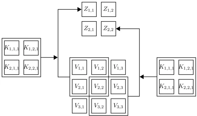
The convolutions used for neural networks in practice are usually different from the stan-dard discrete convolution [1]. Usually, many convolutions are applied in parallel to extract different kinds of features, for example different kinds of edges in the same region of an image. These different convolutions are also referred to as filters or channels. The input itself is often not just a grid but a grid of vectors. To illustrate this on an example, assume we have 2-D data V = (Vj,k). We want to apply the 3-D kernel tensor K = (Kj,k,l) where

Figure 2.2: Example of a convolution. The 2×2 sized kernel K of the first filter is applied to the 2-dimensional input V ∈_R3×3 _{with stride 1 to produce the 2}_×_{2 sized output} _Z_.

Kj,k,l is the connection of an input unit with the output unit of the j−th filter with an offset ofkrows andl columns between output and input unit (see Fig. 2.2 for an example).

(26)

Therefore output Z = (Zj,k) can be written as

Zj,k = X

j,m,n

=Vl,j−1+m,k−1+nKl,m,n. (2.10) For the convolution operation, we can also skip over some positions of the kernel in order to reduce computational costs. With stride s (sample only every s pixels) we have

Zj,k = X

j,m,n

=Vl,(j−1)s+m,(k−1)s+nKl,m,n. (2.11)

Another essential feature of convolution is zero padding the input V (adding rows and

columns of zeros at the margins). As the width of representations shrinks every layer when using convolutions, zero padding allows control over the kernel width and the size of the output independently without having to choose between fast shrinking of dimensions or small (enough) kernel sizes.

2.4 Initialization, Regularization and Optimization

2.4.1 Weight Initialization

Training deep learning models with current techniques is an iterative procedure and re-quires an initial set of values. These values can have a substantial impact on the speed of convergence, the quality of the found solution and the occurence of numerical difficulties [1]. It is not yet well defined which properties initial values should possess, therefore most initialization strategies are simple and heuristic [1]. One well-known property, however, is symmetry breaking. When initialized with the same weights, units with similar inputs and activation functions will, in essence, learn the same representation [1]. Initializing weights by sampling from a high entropy distribution is both cheap and unlikely to assign the same initial values. Popular choices are the uniform and the Gaussian distribution. Biases are typically set to values that are chosen heuristically [1].

2.4.2 Early Stopping

Early stopping is the most common form of regularization and requires almost no change in the training process [1]. When training models with a large effective capacity, over-fitting can occur. This can be counteracted by early stopping. The idea is to monitor the generalization error during the training phase and stop training if the generalization error is increasing or has not decreased for a certain amount of time or update iterations. Monitoring the generalization error requires a validation set, which cannot be used for training. In cases where little data is available for training, this may be rather undesirable. However, there are strategies to still make use of the validation data during training (see [1] for details).

(27)

2.4 Initialization, Regularization and Optimization 15

2.4.3 Dropout

Dropout [64] is a regularization method that is applicable for almost all models using distributed representation. It is computationally inexpensive as well as powerful [1]. In bagging, a number of different data sets are created by sampling with replacement from the original data set. Subsequently, the same number of models are trained, where one model is trained on exactly one data set. Dropout can be seen as an approximation of training (and evaluating) a bagged ensemble of exponentially many neural networks [1]. For each batch of data during training a kind of binary mask is randomly created. This binary mask determines for each input unit and hidden unit whether it is included or not. The binary values are sampled independently with a predefined probability (which is therefore a hyperparameter). The mask for each batch is independent from all the other masks created. In some sense, an ensemble of all sub-networks of the original network is trained. For a more in-depth introduction to dropout, please refer to [1]. Dropout has proven to be more effective than other standard computanionally inexpensive regularizers such as weight decay [64]. Although the actual cost of applying dropout during training is low, the cost for the complete system might end up being significant [1]. As dropout is a form of regularization, it reduces the effective capacity of the model and may therefore create the need to increase the model size, resulting in a potentially more expensive training and evaluation process.

2.4.4 Batch Normalization

Batch normalization [65] is an optimization technique that is actually not an algorithm but an adaptive reparameterization method. Deep models consist of a hierarchy of layers and their training involves updating certain weights. In some sense, the gradient update of the parameters is done under the implicit assumption that the weights of the other layers do not change when, in reality, the layers are actually updated simultaneously [1]. Batch normalization reduces the problem of coordinating these updates. It can be applied to individual input and hidden layers. The idea behind it is to reparameterize the activations of a layer for a given batch update by subtracting the mean and dividing the result by the standard deviation. Note that the output of each neuron is reparameterized separately and the mean and standard deviation are computed with respect to the different values coming from the batch data. An important point is that the back-propagation should also go through these operations. For more information on batch normalization please see [1].

2.4.5 Momentum

Training a neural network with SGD can be slow. Momentum is an optimization technique designed to improve the amount of required training time for high curvature (of the objec-tive function w.r.t. the parameters), small and consistent gradients and noisy gradients. The idea of momentum can be explained informally by using the analogy of a ball rolling through the space that should be optimized. At a given moment, the negative gradient at

(28)

the position of the ball gives the direction of steepest descent and therefore the direction in which the ball tends to roll. However, it does not always roll in the direction of the negative gradient since it may be in motion rolling towards a direction given by previous negative gradients pointing in other directions than the current one. Furthermore, if the descent is rather flat but always points in the same direction, the ball picks up more and more speed along the way. More formally, the step update is not only the negative gradient multiplied by the learning rate but also includes a exponentially decaying moving average of past gradients. Let α∈[0,1), ∈[0,1) (learning rate) and gθ denote the gradient at θ. Then

v ←αv−gθ, (2.12)

θ←θ+v. (2.13)

The hyperparameter α determines how quickly the contribution of v decays. For a more

thorough introduction to momentum, please refer to [1].

2.5 Hyperparameter Selection

A large part of deep learning algorithms have many hyperparameters that influence a ma-jority of its behaviour concerning computational time, memory resources and the resulting model quality (in terms of the ability to generalize) [1]. Hyperparameters can be chosen either automatically or manually. Manual selection requires a thorough understanding of how the learning algorithm works and the hyperparameter’s influence on this process while automatic selection may require less knowledge about the algorithm but more computa-tional resources.

2.5.1 Manual Hyperparameter Tuning

To achieve good generalization of the model, the primary goal in manual hyperparameter tuning is to adjust the effective capacity of the model according to the complexity of the application. The effective capacity of the model describes the ability of the model to capture increasingly complex relationships between the representation and the target. It is constrained by the representational capacity of the model (what relationships could be captured), the learning algorithm’s ability to minimize the cost function (if the model is trained in a suboptimal way it may not utilize its full capabilities) as well as regularization. The generalization error as a function of the hyperparameters typically follows a U-shaped curve [1]. On one end of the spectrum, the effective capacity is very low, which leads to underfitting and hence a high training error as well as a high generalization error. On the other end of the spectrum, the effective capacity is too high, resulting in overfitting. This shows in a low training error but a high generalization error. Some hyperparameters cannot explore the entire U-shape of the curve. Discrete hyperparameters, for example, can only

(29)

2.5 Hyperparameter Selection 17 capture a finite set of points. Other hyperparameters may have boundaries preventing them, such as regularization hyperparameters, which can usually only substract capacity and are therefore likely to be bounded in (at least) one direction. The learning rate is a hyperparameter of particular interest, as the training error is a U-shaped function of the learning rate. When too high, it can even increase the training error and values that are too small can slow training down significantly or lead to stagnation of the training error. It may therefore be the most important hyperparameter with respect to finding a suitable value [1]. Usually, a large, well regularized model is among the most performant ones [1]. When the training error is low, another approach to achieve good generalization is to use more training data. This approach is more of a brute-force nature and comes with an increase in computational expenses.

2.5.2 Automatic Hyperparameter Tuning

Ideally, the deep learning algorithm receives data and computes a desired output with-out any manual tuning. Neural networks, however, often have a lot of hyperparameters and may benefit substantially from tuning them [1]. In most instances, tuning manually requires expertise and experience, both of which are not always present for every appli-cation. Tuning hyperparameters can be viewed as an optimization problem where the generalization error is optimized with respect to the hyperparameters. Algorithms for tun-ing hyperparameters can have hyperparameters themselves, e. g. search ranges, but these are usually easier to choose as similar choices work well for a wider range of tasks.

Grid search is a simple approach where the user selects a finite set of values for each hy-perparameter. The model is then trained with every setting of the Cartesian product of these value sets to find the one with the best generalization. Note that as the set for each hyperparameter should be finite, the user needs to provide a discrete selection of sample points also for continuous hyperparameters. The result of using the grid search algorithm can be improved when it is applied repeatedly, where the next grid is placed around the current best setting. A major drawback of grid search are the high computational costs, as they grow exponentially with the number of hyperparameters. This can be lessened to some extent by using parallelization since there is almost no communication needed between different entities evaluating the search grid.

Random Search is comparably simple to implement, arguably more convenient to use and converges faster to favorable values [20]. Sample points are chosen according to a prede-fined probability distribution (e. g. a uniform distribution). Unlike grid search, continuous hyperparameters are not discretized which results in the exploration of a larger set of val-ues without adding computational costs. Furthermore, less experiment runs are wasted [1]. When the influence of two different values for a hyperparameter only differs marginally, the setting is effectively run twice in grid search as the algorithm will evaluate both values with similar values of the remaining hyperparameters. This is unlikey to happen in a practical setting with random search if both values of the hyperparameter in question are evaluated as the remaining hyperparameters are unlikely to be the same.

(30)

non-differentiability of certain components. A derivative-free optimization approach is MBO, where the generalization error (or value of some performance measure) is modeled w.r.t. the hyperparameters. A new proposal is then made based on optimizing within the model. A common technique for determining the relevance of a new proposal is to consider both the expected generalization error as well as the model’s uncertainty around the expectation.

(31)

Chapter 3 Model-Based Optimization

3.1 History of Model-Based Optimization

The following overview of the origins of MBO is drawn primarily from [15].

An early work (and possibly the earliest according to [15] and [66]), incorporating an ap-proach that resembles MBO is [67] using Wiener processes for searching a one-dimensional and unconstrained parameter space. The Wiener process interpolates the data points lin-early in a piecewise manner with a quadratic variance model which is zero at each sample [66]. Kushner discussed the weakness of local optimizers (in particular gradient-based op-timization algorithms) regarding converging to local optima and argued that it would be desirable to have the algorithm search the entire parameter space for each iteration. Similar to MBO, the approach of [67] proposes that the points are chosen sequentially according to the maximization of an improvement criterion, namely the probability of improvement (see Subsec. 3.5.1), and including a component that incorporates a trade-off resembling the exploration-exploitation trade-off (see Subsec. 3.2). This technique was later extended, e. g., in [68, 69]. A multidimensional MBO approach was published in [70], using linear combinations of Wiener fields and maximizing a critierion similar to expected improvement function (see Subsec. 3.5.2) [15]. A review of this work was published in [71]. Related work was published under the name Kriging (see Sec. 3.4.1). The technique, which was further advanced and primarily made popular by [72] (according to [15]), is named after the South African geologist (and student at the time of conducting his research) D. G. Krige who de-veloped the technique [73]. Its goal is interpolating a random field using a linear predictor, the errors are modelled with a Gaussian process. Krige’s work “formed the foundation for an entire field of study now known as geostatistics” [66] (see, e. g., [74, 75]). In the late 1980s, Kriging was applied to deterministic computer experiments [76, 77]. The resulting approach was named Design and Analysis of Computer Experiments (DACE). Specific techniques used in DACE deviated from the geostatistical approach in concentrating on a “small” part of the knowledge available [66]. MBO using Gaussian processes has been applied in the discipline of experimental design (see Sec. 3.6), for example by Jones et al. [30] who proposed a SMBO algorithm called Efficient Global Optimization (EGO) (see

(32)

Sec. 3.6). Several consistency proofs for variants of this algorithm exist ([78, 79]).

3.2 General Framework

MBO or Bayesian optimization is a powerful strategy for optimizing black-box functions that is very efficient in terms of required function evaluations (see [15]). Let f : X → _R

denote a black-box function, where the input space is X = X1 ×X2 ×...× Xd. For

i ∈ {1, ..., d}, Xi can either represent the domain of a categorical variable with finitely many values Xi = {vi1, ..., vit}, t ∈ N, or the domain of a bounded numeric variable

Xi = [li, ui], li ∈ R, ui ∈ R and li < ui. Since f should be optimized, we can assume without loss of generality that f should be minimized, so essentially the goal is to find x∗

such that

x∗ = arg min x∈X

f(x). (3.1)

We assume thatf is expensive to evaluate, limiting the number of function evaluations by a budget.

Let Ds = {xi, f(xi)|i ∈ {1, ..., s}} for s ∈ N. In MBO, the knowledge of Ds is incor-porated using Bayes’ theorem (which explains the term Bayesian optimization) to improve the assumed distribution over the space of objective functions:

P(f|Ds)∝P(Ds|f)P(f). (3.2)

P(f) is theprior, representing the belief about the space of objective functions. P(Ds|f) is thelikelihood, representing how likely the present data is given the belief about the function space. P(f|Ds) is the posterior, essentially representing the updated belief about function space after observingDs. Every update, prior knowledge and evidence is used to maximize the posterior, so each evaluation decreases the distance between the true optimum of f

and the expected optimum of f using the posterior P(f|Ds) [15]. An informative prior can be used to express belief or knowledge about attributes of the objective function like the most likely locations of the maximum, even without actually knowing the function [15]. In practice, the generic SMBO algorithm looks as follows (see, e. g., [16]):

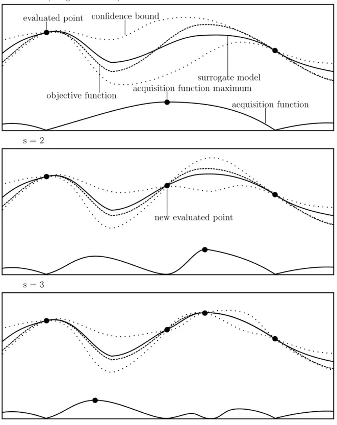
In the beginning, an initial design is generated by sampling points fromX and evaluating

f at these points. In each iteration, the objective function is (cheaply) estimated with a surrogate model (see Sec. 3.4). An acquisition function (see Sec. 3.5) is then used to effi-ciently determine the next sample location, as can be seen in Algorithm 1. The acquisition function is defined on X and utilizes the surrogate model. It represents a trade-off be-tween exploration (sample points in areas with high uncertainty aboutf) and exploitation

(sample points at or near the expected optimum of f), for example by taking the mean

and the variance of the surrogate model into account. The acquisition function is usually easy to optimize (see [15]) and its optimum gives the point of the next evaluation of the

(33)

3.2 General Framework 21

evaluated point confidence bound

objective function

surrogate model

acquisition function acquisition function maximum

new evaluated point s = 1 (design size k = 2)

s = 2

s = 3

(34)

Algorithm 1 Sequential Model-Based Optimization.

1: Generate initial design D0 ={(xi, f(xi))|i∈ {1, ..., k}, xi ∈X}, k ∈N.

2: for s= 1,2, ...do

3: Fit a regression model (the surrogate model, see Sec. 3.4) to Ds−1.

4: Use the model to determine xs (often by optimizing an acquisition function, see

Sec. 3.5).

5: Evaluate f atxs to obtain f(xs).

6: Define Ds =Ds−1∪ {xs}.

objective function. See Fig. 3.1 for an example. The SMBO algorithm terminates when a predefined termination criterion is fulfilled. This can, for example, be a total number of evaluations of f or SMBO iterations, a time budget for evaluations of f, or reaching a certain objective value. SMBO is modular and the generic approach can be extended in various ways, e. g. optimizing an objective function f with multi-dimensional output [80] [16] or proposing multiple points for one iteration of s in Algorithm 1 [81, 82].

3.3 Initial Design

The surrogate models are fitted iteratively after new evaluations of f. To fit an initial surrogate model (for s = 0 in Algorithm 1), an initial design {(x1, f(x1)), ...,(xk, f(xk))} consisting of sampled values of X and the corresponding evaluated values of f is created. Choosing the initial design may affect the optimization process, as for example a large initial design may result in an undesired amount of computing time or function evaluations for points that are not part of the actual optimization process (in the sense that they do not optimize the acquisition function at some stage). Conversely, a small design may result in a poor fit of the surrogate model and consequently suboptimal proposals for the next

points to evaluate. This may also occur if the design does not cover X appropriately.

One way to generate an initial design is to use space-filling Latin Hypercube Designs [83], which ensures that all portions of the range are represented adequately for every input variable. Additionally, they are computationally cheap to generate and can handle many input variables [76]. Possible choices for the size of the design are 2∗d and 4∗d, whered

denotes the number of tuned hyperparameters.

3.4 Surrogate Model

Surrogate models provide a functional relationship to the objective function while being computationally favorable (see [66]). A deciding factor for the choice of the surrogate model is the structure of the input space X. For input spaces with exclusively numeric variables (X ⊂_R), Kriging (see Sec. 3.4.1 and Sec. 3.6) provides state-of-the-art performance and is hence recommended [16]. In practice, the parameter space rarely consists solely of numeric parameters, but often contains categorical parameters as well as hierarchical dependencies

(35)

3.4 Surrogate Model 23 resulting in conditional parameters. For search spaces that include categorical variables,

random forests [43] can be used to model f without encoding categorical variables as

(discrete) numeric variables. The Kriging approach can be extended for hierarchical input spaces by utilizing suitable kernel functions for both numeric and categorical variables [31], but this is still an ongoing process of research [32]. However, random forests are again a viable alternative. Hereafter, let ˆf denote the surrogate model.

3.4.1 Kriging and the Gaussian Process

Originally developed by Krige [73] for analyzing mining data using statistics-based tech-niques, Kriging has provided a basis for and been used in geostatistics since the 1950s [66, 15]. Detailed introductions and examinations can be found in [84, 66, 85]. An al-ternative introduction to Kriging is given in [86]. While limited to a numeric-only input domain, Kriging is still arguably the most popular choice for surrogate models as it pro-vides both flexibility and a local uncertainty estimator [16]. Assume we have observations

{(xi, yi)|i ∈ {1, ..., k}} consisting of input xi and corresponding output yi = y(xi) and that their relationship is given by

y(x) = f(x) +. (3.3)

In contrast to many machine learning models, the usual assumption in Kriging is that the residuals are not independent and identically distributed iid∼ N(0, σ2

) but a function of

x. They are assumed to be spatially correlated in the sense that the if error i for sample point xi is high, the errors for sample points near xi are expected to be high as well. Therefore, in its essence, Kriging combines linear regression with a stochastic model fitted to the resulting residuals, namely(x)∼ N(0, σ2(x)). The type of linear regression model is determined by the type of Kriging method used and can range from the zero function (simple Kriging) to a polynomial function (universal Kriging) and other models.

The GP is an extension of the multivariate Gaussian distribution. It is a stochastic process with infinite dimensions where any finite subselection of dimensions follows a multivariate Gaussian distribution [15]. A GP can be viewed as a distribution over functions, analogous to a Gaussian distribution being a distribution of a random variable over its possible values. Furthermore, just as a Gaussian distribution is specified by its mean and covariance, a GP is specified by its mean function and covariance function. Intuitively, it can be useful to think of a GP as a function, which returns the mean and variance of a Gaussian distribution over the possible values for the input valuex [15].

While Kriging and MBO are closely related, there are some key differences in practice regarding the way models are fitted (see, e. g., [15, 66]). However, the term Kriging often refers to MBO with a GP surrogate model. For a more in-depth introduction to Kriging see, e. g., [86].

(36)

3.4.2 Random Forest

A random forest (RF) for regression is a model which consists of a large collection of regression trees [87]. Regression trees are similar to decision trees but return a numeric value rather than a categorical value [43]. A prediction value is produced by aggregating the individual results in a suitable fashion. Regression trees can capture complex interactions in the data and have relatively low bias if grown sufficiently deep [87]. As the covariates are selected randomly in the tree-growing process, the correlation between the trees is reduced without increasing the variance too much. Regression trees can handle categorical input variables well. This property transfers to RFs, which, in addition, usually yield more accurate predictions than regression trees [43].

An algorithm of a RF for regression can be found in [87]: 1. For b = 1 to B:

(a) Draw a bootstrap sample Z∗ of size N from the training data.

(b) Grow a random forest tree Tb to the bootstrapped data by recursively repeating the following steps for each terminal node of the tree until the minimum node size nmin is reached.

i. Select m covariates at random from the p covariates. ii. Pick the best covariate split-point among them. iii. Split the node into two child nodes.

2. Output the ensemble of trees {Tb}B1.

A prediction at a new point x is made via aggregation: ˆ f_rfB(x) = 1 B B X b=1 Tb(x). (3.4)

Note that in order to use certain acquisition functions (see for example Subsec. 3.5.2 and Subsec. 3.5.3), an uncertainty estimate needs to be computed. While this can be achieved in multiple ways, the jackknife estimator works reliably according to [16]. As the random forest is not a spatial model and does not come with a native uncertainty estimate out-of-the-box, the computed estimate is less intuitive in contrast to the Gaussian Process.

3.5 Acquisition Function

The purpose of the acquisition functionu, also called infill criterion, guides the optimization process in the sense that for a given surrogate model, its optimum is proposed as the next evaluation point for the objective function f. Therefore, the desired point is either

arg max x∈X

(37)

3.5 Acquisition Function 25 or

arg min x∈X

u(x|Ds), (3.6)

depending on whether the acquisition functionuis maximized or minimized. Conditioning on Ds refers to ˆf(x|Ds), which is the surrogate model fitted to the available evaluations

Ds of f. The acquisition function typically also contains some trade-off between explo-ration, sampling points in regions with high uncertainty, and exploitation, sampling points in regions with favorable values of the surrogate model, by combining the posterior mean ˆ

µ(x|Ds) and the posterior deviation ˆs(x|Ds) or the posterior variance ˆs2(x|Ds) in a suit-able formula. Under the assumption that high values of ˆs(x|Ds) suggest that few of the evaluated points lie in or close to the region of concern, points with high values of ˆs(x|Ds) are of interest. Additionally, these points should have low ˆµ(x|Ds) when minimizing and high ˆµ(x|Ds) when maximizing the acquisition function (see [16]). As there are several ac-quisition functions, it can be unclear which one to use. Broch et al. [88] propose a method of utility selection where a portfolio of acquisition functions combined with a multi-armed bandit strategy is used instead of a single acquisition function.

3.5.1 Probability of Improvement

Kushner [67] suggested using the probability of improvement (PI) as the acquisition func-tion. Note that in this case, the acquisition function should be maximized. For a max-imization of the objective function and a GP as a surrogate model the probability of improvement is PI(x) = P(f(x)≥y_max(s) ) (3.7) = Φ µˆ(x|Ds)−y (s) max ˆ s(x|Ds) ! , (3.8)

with ymax(s) = max{f(xi)|(xi, f(xi)) ∈ Ds} the best evaluated value observed so far and Φ(·) the cumulative distribution function of the Gaussian distribution. However, this formulation puts great emphasis on exploitation. Points that potentially result in a high improvement but with a high uncertainty are unfavored in comparison to points that offer little improvement with high certainty. To regulate exploration and exploitation, the trade-off parameter ξ≥0 can be added (see [15]):

PI(x) = P(f(x)≥y(s)_max+ξ). (3.9)

In this setting, greater values of ξ put greater emphasize on exploration and vice versa. However, as Jones [86] points out, the emphasis on exploration or exploitation is highly sensitive to the choice of ξ, therefore choosing a suitable ξ may be a difficult task. For a more detailed analysis of the probability of improvement, please refer to [86].

(38)

3.5.2 Expected Improvement

A popular (and arguably the most popular according to [16]) acquisition function is the expected improvement (EI). In contrast to the PI, the EI criterion takes the magnitude of the potential improvement into account. The expected improvement can be defined as

EI(x) = E(I(x)), (3.10)

where the random variable I(x) is the potential improvement at x over the current opti-mum. In the case of minimizing the objective function this is

I(x) = max{y_min(s) −Y(x|Ds),0}, (3.11)

where y(s)_min = min{f(xi)|(xi, f(xi)) ∈ Ds} and Y(x|Ds) is a random variable represent-ing the posterior distribution at x. When usrepresent-ing a Gaussian process, Y(x|Ds) follows a Gaussian distribution, Y(x|Ds) ∼ N(ˆµ(x|Ds),ˆs2(x|Ds)). In this case, let Φ and φ be the distribution and the density function of the Gaussian distribution, respectively. Then EI can be expressed as (see [30, 16])

EI has proven to be a well-balanced and highly effective acquisition function [30] and can even ensure global convergence [89].

3.5.3 Confidence Bound Criteria

A pragmatic approach to combine ˆµ(x|Ds) and ˆs(x|Ds) is to use a confidence bound as the acquisition function. For minimizing the objective function, the lower confidence bound is

LCB(x) = ˆµ(x|Ds)−λˆs(x|Ds), (3.13)

with λ≥0 balancing the trade-off between exploration and exploitation. Higher values of

λ put higher emphasis on exploration and vice versa. The special case λ = 0 illustrates the case in which all emphasis is put on exploitation. Analogously, the upper confidence bound for the case of maximizing the objective function is

UCB(x) = ˆµ(x|Ds) +λˆs(x|Ds). (3.14)

3.5.4 Expected Improvement per Second

The main objective of applying MBO to tuning is to find a good setting of hyperparameters. Acquisition functions like EI are greedy in the sense that at every iteration the next proposal

(39)

3.6 DACE and EGO 27 (ideally) yields the best progress in terms of the acquisition function. Snoek et al. [23] argue that most of the time in practice the concern is not to make progress in as few iterations as possible, but rather to make progress in as little time as possible. They therefore suggest to use the expected improvement per second as the acquisition function. Let c(x) denote the duration function that gives the duration of evaluating the objective function f for a set of hyperparameters x. Most likely, c is a black-box function as well. Snoek et al. propose to model log(c) using a Gaussian process. Under the assumption that

c and f are independent, one can compute the predicted expected inverse duration easily and hence the expected improvement per second.

3.5.5 Optimizing the Acquisition Function

To propose the next evaluation point forf, the acquisition function needs to be optimized. One characteristic of the acquisition function u(·) is that samples can be attained cheaply. While still a black-box optimization problem, this drastically simplifies the optimization in contrast to the objective function. Various approaches for optimization exist, like the branch and bound algorithm proposed by Jones et al. [30] or the multistart approach by Lizotte [90]. Another alternative is thefocus search approach proposed by Bischl et al. [16].

3.6 DACE and EGO

DACE was introduced by Sacks et al. [76] and is a discipline focused on solving problems posed by the optimization task of a black-box function [16]. In this context, a computer experiment is defined as running a computer model or code a number of times with various inputs. The output of the code is assumed to be deterministic, i. e., rerunning the model with the same input parameters should yield the same output. For optimization, an efficient predictor should be fitted to the evaluated input values and the corresponding deterministic output to predict the output at untried inputs. To achieve this, the deterministic output is modelled as the realization of a stochastic process. This provides a statistical basis for choosing input parameters of the experiment as well as an estimate of uncertainty for the model’s prediction. Indeed, DACE is Kriging (with a specific kind of kernel, see, e. g., [90, 30]) applied to experimental design [15].

The EGO algorithm introduced by Jones et al. [30] is a SMBO approach that combines the DACE model with the EI as acquisition function (see, e. g., [15, 90]). EGO is limited to optimizing noise-free functions with real-valued parameters [43]. Nonetheless, it has proven to be highly effective [16]. Since the publication of EGO, several extensions to the algorithm have been made (see, e. g., [66, 91]).

Configuration of Deep Neural Networks Using Model-Based Optimization

Ludwig-Maximilian University of Munich

Master Thesis