The Selective Decision Tree Classifier: A Novel Classifier based on Feature Selection

(1)

The Selective Decision Tree Classifier:

A Novel Classifier based on Feature Selection

A Thesis Submitted to the

College of Graduate and Postdoctoral Studies

in Partial Fulfillment of the Requirements

for the degree of Master of Science

in the Department of Computer Science

University of Saskatchewan

Saskatoon

By

Jennafer Neiser

(2)

Permission to Use

In presenting this thesis in partial fulfilment of the requirements for a Postgraduate degree from the University of Saskatchewan, I agree that the Libraries of this University may make it freely available for inspection. I further agree that permission for copying of this thesis in any manner, in whole or in part, for scholarly purposes may be granted by the professor or professors who supervised my thesis work or, in their absence, by the Head of the Department or the Dean of the College in which my thesis work was done. It is understood that any copying or publication or use of this thesis or parts thereof for financial gain shall not be allowed without my written permission. It is also understood that due recognition shall be given to me and to the University of Saskatchewan in any scholarly use which may be made of any material in my thesis. Requests for permission to copy or to make other use of material in this thesis in whole or part should be addressed to:

Head of the Department of Computer Science 176 Thorvaldson Building 110 Science Place University of Saskatchewan Saskatoon, Saskatchewan Canada S7N 5C9 Or Dean

College of Graduate and Postdoctoral Studies University of Saskatchewan

116 Thorvaldson Building, 110 Science Place Saskatoon, Saskatchewan S7N 5C9

(3)

Abstract

Living in the era of big data, it is crucial to develop and improve techniques that aid in data processing, such as data reduction. Feature selection is a data reduction technique that generates subsets of data that can be used to build machine learning models. Machine learning utilizes the processing power of a computer to build classification models from the inputted features. By pre-selecting the most relevant features in a data set, machine learning techniques can build simpler and more accurate models.

A novel method of classification based on feature selection is proposed, the Selective Decision Tree classifier (SDTC). The SDTC is derived from the Selective Bayesian classifier (SBC). Both classifiers use Decision Trees (DTs) to rank the features of a data set. DTs are built to organize features in a tree structure, with the most predictive features at the top of the tree, branching down into features that eventually lead to a classification. Features are evaluated and ranked into the levels of the DT. Both classification methods select features from the upper levels of a DT, and those features are fed into a machine learning model built to classify data. The SDTC allows for different depths of levels to be selected, whereas the SBC uses a fixed depth of three levels. To allow for greater scalability of data sets, the SDTC uses DTs as the final machine learning model, whereas the SBC uses the Naive Bayesian model.

The SDTC is applied to three data sets. The first data set is the Level of Service Inventory (LSI) data set that details over 72,000 responses to a recidivism risk assessment test and whether those individuals recidi-vated. The second data set is provided by the Saskatoon Police Service and contains information on missing children cases. The third data set provides the scores and reaction times recorded from the Computerized Assessment of Mild Cognitive Impairment (CAMCI) test taken by individuals as a pre-diagnostic tool for Alzheimer’s disease and dementia. To demonstrate where the SDTC excels at building better predictive models, two other classification models were built from the data sets, DTs and the SBC.

When comparing the SDTC to a DT model, the advantages of feature selection are clearly evident as demonstrated by the improved accuracy. Using the LSI data set, the SDTC selected a single feature out of 43 and obtained over a 76% accuracy, compared to the 71% accuracy obtained by a DT model using all the features. The highest accuracy, 92%, was seen using the SDTC on the Missing Persons data set, almost a 7% increase using only two of the 90 features when compared to DTs. Using the CAMCI data set, the SDTC achieved a 60% accuracy using only 12 of the 33 features, compared to a 58% accuracy obtained by DTs using all the features. The flexibility of the SDTC also gave it distinct advantages and in some cases improved accuracy in its predictive potential when compared to SBC. The SDTC outperformed the SBC on two of the three data sets. The highest increase in accuracy when comparing the SDTC and the SBC was obtained using the Missing Persons data set; the SDTC achieved 92% accuracy, a 7% higher accuracy than the SBC. The demonstrated capability of the SDTC supports its potential for analyzing a variety of data sets and obtaining a deeper understanding of how DT structures can be used for feature selection.

(4)

Acknowledgements

I would like to acknowledge the support of the Computer Science Graduate Studies Department for their constant help and knowledge provided. I would like to acknowledge my parents for the support they provided me through constant love and words of perseverance. I would like to thank my husband, Brandon, for his constant patience and encouragement during the many hours of writing and research. I would like to thank my supervisor Dr. Raymond J. Spiteri. I would also like to recognize the agencies that provided me and the team I work with ethical access to the data worked with in this thesis: Ontario Ministry of Community Safety and Correctional Services, Saskatoon Police Services, Psychological Software Tools, Inc. (Pittsburgh, PA), the Psychology Department at the University of Saskatchewan, and the Centre for Forensic Behavioural Science and Justice Studies at the University of Saskatchewan.

(5)

List of Tables

3.1 Re-offense Raw Data Table for Naive Bayesian Example . . . 20

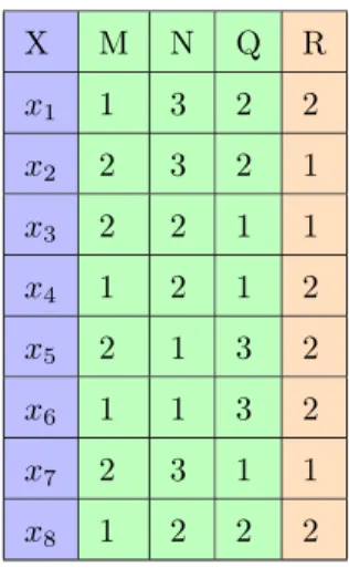
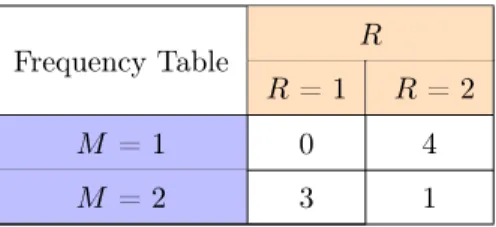
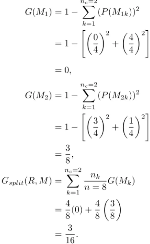
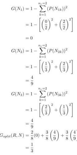
3.2 Frequency Table . . . 21

3.3 Raw Data . . . 25

3.4 Target Feature . . . 25

3.5 Frequency Table . . . 26

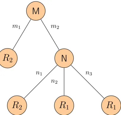
3.6 Raw Data for Gini Example . . . 28

3.7 Frequency Table forM . . . 29

3.8 Frequency Table forN . . . 30

3.9 Frequency Table forQ . . . 31

4.1 SDTC Results for LSI Data . . . 41

4.2 The Overlay of Features Selected at Depth 3 . . . 42

4.3 Statistics for the Best Selected Model and the Original Full Model in Percent (%) . . . 42

4.4 LSI-R:SV Comparison (%) . . . 44

4.5 LSI-R:SV Feature Comparison . . . 44

4.6 SDTC Results formissing_again . . . 46

4.8 SDTC Results forgang_involvment . . . 49

4.10 SDTC Results for CAMCI . . . 53

(8)

List of Figures

3.1 Decision Tree Classification . . . 23

3.2 A DT Example . . . 23

3.3 DT Model Produced from Gini DT Method . . . 33

3.5 Selective Bayesian Classifier (Ratanamahatana and Gunopulos,2002) . . . 35

3.6 A DT Example . . . 36

4.1 Confusion Matrix (Townsend,1971) . . . 39

4.2 Re-offence Distribution . . . 40

4.3 Total Score Distribution . . . 40

(9)

List of Abbreviations

AD Alzheimer’s Disease AUC Area Under the Curve

CAMCI Computer Assessment of Mild Cognitive Impairment CART Classification and Regression Tree

CT Classification Tree DT Decision Tree Classifier LSIT Latest-Substring Index Tree LSI Level of Service Inventory

LS/CMI Level of Service/Case Management Inventory

LSI-R:SV Level of Service Inventory - Revised: Screening Version MCI Mild Cognitive Impairment

MMSE Mini Mental State Examination NBD Naive Bayes with Discretization

NBK Naive Bayes with Kernel Density Estimation RBFN Radial Basis Function Network

SBC Selective Bayesian classifier SDTC Selective Decision Tree classifier

SPECT Single Photon Emission Computed Tomography SPS Saskatoon Police Service

(10)

1 Introduction

Transitioning from the data explosion era to the big data era leaves many new and ever-changing problems for researchers to face (Cai and Zhu,2015). Data scientists are no longer working with data units of GB or TB, but larger units like PB (1 PB = 210 _{TB), EB (1 EB}_{= 2}10 _{PB), and ZB (1 ZB} _{= 2}10 _{EB). A major}

challenge when working with big data is ensuring the quality of the data and consequently any models built with the data. The more data under consideration, the harder it is to judge data quality within a reasonable amount of time (Cai and Zhu, 2015). Data analytics plays a part in the processing of big data to improve the data quality. By improving data quality, the efficiency of data utilization will increase, and the risk of poor classification models being built and used will decrease.

When working with a data set that has many features (high dimensionality), there can be features that do not add to the predictive power or accuracy of a model. Features that do not contribute to the overall accuracy of a model are redundant and ultimately unneeded. Neglecting to remove irrelevant or redundant features can lead to over-fitting and longer training times for machine learning models (Brownlee, 2016b). Also, working with smaller groups of selected features often leads to simpler models that are easier to interpret. Accordingly, feature selection is often an important process to perform on big data sets to help improve the quality of the data for the classification models being built.

This thesis explores a novel classification method based on selecting the most important features from a data set: the Selective Decision Tree classifier (SDTC). The SDTC is derived from a technique called the Selective Bayesian classifier (SBC) (Ratanamahatana and Gunopulos,2002). The SDTC first uses Decision Trees (DTs) to determine which features of a data set are the most important. Using only these selected features, a DT is applied a second time to build a final classification model. The goal is that minimal prediction accuracy is lost and the number of features used to build a classification model is reduced. By achieving this goal over multiple data sets, the argument that SDTCs are a valid way to improve data quality is strengthened. Also by applying the SDTC to the three data sets used in this thesis, advances in usable prediction models and feature understanding can be made in those areas of study.

1.1 Machine Learning

Since the beginning of the computer era, machine learning has been used to discover facts and theories about data by enhancing predictive tests (Michalski et al.,2013). There are many trusted machine learning methods that have been developed, e.g., DTs (Quinlan, 1993, 1986), Naive Bayesian classification (Elkan,

(11)

1997), and Support Vector Machines (Gunn et al., 1998). Machine learning methods can be used to build models that classify data; those classifications can be interpreted to inform predictions. DTs are the main machine learning method used in this thesis. A DT is built using a set of data consisting of features; the features are layered into a tree structure that can be used for classification. Where the features are placed in the tree is determined by a splitting criterion. For example, consider a data set that represents a series of responses to a set of questions used to determine whether or not an individual might commit a crime. The questions become the layered features of the DT, and the responses to the questions are the data used to build the DT. The DT model classifies whether or not an individual is likely to commit a crime.

1.2 Feature Selection

Feature selection is the process of eliminating features or dimensionality in a data set while still retaining the accuracy of a model built with the entire data set. Often there are features in large data sets that do not provide meaningful information and can be considered redundant. Removing these features reduces the chances that the model built is over-fit to the data used (Brownlee, 2016b). A model is over-fit when the performance of the model built with the testing data declines greatly when used to classify testing or real world data (Cawley and Talbot,2010). The feature selection method, SDTC, uses DTs to both select features from a data set and to build a final classification model. The SDTC is derived from the SBC (Ratanamahatana and Gunopulos,2002).

1.2.1 Selective Decision Tree Classifier

The SDTC uses DTs for ranking and selecting features and for building the classification model. The SDTC refines the initial steps of the SBC and replaces the final model with a DT. In this thesis, the DT steps were tested with both Gini and Entropy DTs (Buntine and Niblett, 1992; Quinlan, 1993). The difference between a Gini and Entropy DT is that they use different splitting criteria to determine where features are placed in the DT, resulting in different models being built. These two DT splitting criteria have some of the lowest error rates when compared to other DTs using different splitting criteria tested over multiple data sets (Buntine and Niblett, 1992). In this thesis, the results obtained by both DTs exhibited little variation in accuracy, but there was some variation in the features selected.

The SDTC was tested using three different data sets. The results obtained from the SDTC were compared to the results of a DT built with the three data sets. Comparing the results from DTs and the results from SDTCs gives an indication of how well the feature selection method works and whether it is beneficial to use. The SDTC was also compared to the SBC. This comparison shows where the SDTC is an improvement from the SBC and where they perform similarly. The rest of this chapter briefly describes the data sets and highlights the results obtained.

(12)

1.3 Data Sets

Multiple data sets are used to determine the capabilities of the SDTC. The first data set is comprised of recidivism risk assessment scores from the Level of Service Inventory (LSI) test. The second data set is comprised of data collected by the Saskatoon Police Service (SPS). The final data set is comprised of test scores from the Computerized Assessment of Mild Cognitive Impairment (CAMCI).

1.3.1 LSI

In this thesis and generally speaking, recidivism is referred to as the tendency of a convicted criminal to re-offend. Recidivism risk assessment tools are designed in an attempt to take into consideration the many variations in human behaviour when predicting the likelihood of an individual to re-offend (Andrews and Bonta,2010). TheLevel of Service/Case Management Inventory (LS/CMI) recidivism risk assessment tool was used in Ontario, Canada, from 2010 to 2011, and the results were recorded for72,726individuals. These

records make up one of the data sets used in this thesis. The LS/CMI is known generally as the LSI tool because it is one of many variation of the tool. The LS/CMI is comprised of 43 yes/no questions that are used to determine a risk score (Andrews et al.,1995). The higher the score obtained with the LSI tool, the greater the risk of an individual to re-offend. Questions in the data set are referred to as features and have a binary value of 1 for yes or 0 for no. The SDTC is applied in an attempt to reduce the number of features that are required to accurately provide a risk score.

The 43 LSI features are grouped into eight categories: Criminal History (8features), Education/Employment

(8 features), Family/Marital (4 features), Leisure/Recreation (2 features), Companions (4 features),

Sub-stance Abuse (8features), Pro-Criminal Attitudes (4features), and Antisocial Pattern (4features) (Andrews and Bonta, 2010). The number of features in each category can be interpreted as the importance of that category; i.e., a larger number of questions in a category correlates to a heavier impact that category has on the total score.

1.3.2 Missing Youths

SPS is in the process of implementing the Saskatchewan Police Predictive Analytics Lab (SPPAL) in part-nership with the Ministry of Corrections and Policing and the University of Saskatchewan. The purpose of this lab is to aid the officers and community safety partners in their normal duties by providing user friendly predictive analytics tools to them. The lab is currently working on an inaugural project on Missing Persons. The data provided by the SPS contained 434 missing youths cases with 91 features for each case. The data used with the SDTC were obtained from the provided Missing Youths Database located in the SPPAL.

(13)

1.3.3 CAMCI

The CAMCI is a mild cognitive impairment test administered as a computerized tool. A patient performs a series of tests on a tablet while the program records scores and reaction times for each of the tests (Saxton et al., 2009). CAMCI is a computerized version of paper-and-pencil tests combined with a virtual reality shopping trip where the patient must remember a series of tasks. CAMCI is intended for older individuals who have not been previously diagnosed with a mild cognitive impairment. In total, the test takes on average 1484 seconds or 24.73 minutes to complete; a long time for a clinician to administer a test to a single person. The goal is to derive the key features of the CAMCI test to allow for a shorter pre-diagnostic tool.

The data set used contains 33 features and 580 cases. The data are obtained from Psychological Software Tools, Inc. (Pittsburgh, PA), and the participants were adults living in western Pennsylvania. The features in the data set consist of the reaction times and scores obtained for each test the participant took. There are also features that record the participants age, schooling level, and gender.

1.4 Ethics

Some of the data in this thesis are highly sensitive, and great care was taken to uphold a high ethical standard. The results given in this thesis do not divulge aspects of the data that could be seen as sensitive or proprietary. The University of Saskatchewan ethics file that contains the necessary permissions to work with the data is BEH# 16-166.

1.5 Contributions

The previously discussed data sets were used to test the SDTC. The results obtained from the classification models were interpreted, and the potential advances in the various fields of study were stated. The rest of this chapter briefly discusses the results and how they can benefit the fields of study to which they pertain.

1.5.1 LSI

Working with the data set of LSI scores, the SDTC was used to identify the crucial features, creating a reduced question set. Reducing the question set can improve the ease of tool administration and potentially allow for the re-allocation of resources to individuals according to their risk of recidivism. For example, being able to provide higher-risk individuals with more resources, such as rehabilitation counseling, can lower the chance of an individual recidivating. Another potential advantage is that removing less relevant data can lead to more efficient computations, saving time and resources. A further potential advantage for researchers is that building a model with a smaller set of features can result in the model being simpler, thus easier to understand (Brownlee, 2016a). With a simpler model, a greater number of unspecialized people would be able to interpret the model and how it can be used.

(14)

It was found that there is no loss in accuracy when the SDTC is used compared with the a DT model built with all 43 of the LSI features, demonstrating that the SDTC is a valid way to select features. Using SDTCs, the set of features used to build the model can be reduced to a single feature, for which an accuracy of 76% is obtained, an increase of over 4% from the DT model. The SDTC model also obtained a 33% sensitivity and a 95% specificity, compared to the model built with all features that obtained a 24% sensitivity and a 92% specificity. It is interesting to compare the features selected by the various frameworks of the SDTC tested, as there are many that overlap. Looking at these features, conclusions can be drawn regarding the importance of the features that overlap in the data set.

1.5.1.1 LSI Screening Test

The LSI recidivism risk assessment test has a short form version called the Level of Service Inventory - Revised: Screening Version (LSI-R:SV) used to screen out individuals who are least likely to re-offend (Andrews and Bonta,1998). LSI-R:SV contains a subset of 9 questions or features from the original 43. If an individual scores from 0 to 2 they are at minimum risk, if they score from 3 to 5 they are at medium risk, and if they score from 6 to 8 they are at maximum risk. At minimum risk the full LSI is desirable, at medium risk the full LSI is strongly recommended, and at maximum risk the full LSI is mandatory (Andrews and Bonta, 1998). This test was put together theoretically, but it has not been extensively tested and validated. By comparing the accuracy, specificity, and sensitivity of the SDTC and the LSI-R:SV, the LSI-R:SV can be validated, confirming the features it contains are the most well-suited for the task, or it can be improved using other features selected by the SDTC.

Using the all of the LSI-R:SV features to build a DT, an accuracy of 74% was obtained. The best model built using SDTCs achieved a slightly lower accuracy of 73%. The sensitivity of the LSI-R:SV model was 35% compared to the 15% SDTC obtained. The specificity of the LSI-R:SV model was 92% compared to the 99% SDTC obtained. The features used in the SDTC models and LSI-R:SV varied greatly.

1.5.2 Missing Youths

With feedback and input from the officers at SPS, two questions were asked of the missing youths data. The first being which children, once found, are likely to run away again. Habitual runaways or missing youths make up a majority of the missing youth cases the officers at SPS encounter. The second question asks whether or not a missing child is likely to be involved with gang activity. With answers to these two questions, officers may be able to have a deeper insight into how to approach new missing youths cases and finding the missing children.

Using the SDTC, features were extracted and used to build a predictive model that gives Missing Persons officers possible answers to their questions. The SDTC models built for both questions out performed the DT models built with all 91 features in the data set. For question one, the SDTC model obtained a 92% accuracy, a 79% sensitivity, and a 100% specificity compared to a DT built with all features that obtained a

(15)

84% accuracy, a 73% sensitivity, and a 92% specificity. For question two, the SDTC model obtained an 88% accuracy, a 50% sensitivity, and a 95% specificity compared to a DT built with all features that obtained a 83% accuracy, a 50% sensitivity, and a 90% specificity.

1.5.3 CAMCI

The SDTC was able to obtain a higher predictive accuracy than regular DTs on the CAMCI data set. Each component of the CAMCI test takes different times to complete; the goals were to reduce the total completion time by selecting a subset of components, and to increase the accuracy of the test. To accomplish this, the average time associated with each component was used to determine the length of the test. Each component or piece of the test may have multiple features associated with it, i.e., score or reaction time. If a feature of a component was selected, the average time to complete that component was added to the total time it would take to complete the CAMCI test. It was found that the accuracy could be improved by almost 3% while reducing the time of completion by 3 minutes. The shortest completion time was 14 minutes, reducing the completion time by over 10 minutes, while still increasing the accuracy by 1%. The accuracy of the best SDTC was 59% compared to a DT built with all features that obtained a 56% accuracy. The best SDTC obtained a 75% sensitivity and a 39% specificity. A DT built with all the CAMCI features obtained a 70% sensitivity and a 39% specificity.

1.6 Outline

This thesis contains the research methods used and results obtained when using the SDTC on the LSI data set, the missing youths data set, and the CAMCI data set. Chapter 2 is a summary of other papers that consist of important information to comprehend aspects of this paper. Chapter 3 is a description of the machine learning methods used, including DT and SDTC. Chapter 4 is a write up of the procedures followed to obtain the given results, a detailed description of the data sets used, and a write up and interpretation of the results and how they are beneficial to the various fields the data relates to. Chapter 5 is a summary of the final results and future work.

(16)

2 Literature Review

This section introduces concepts and background information associated with each of the main topics permeating this thesis. Section 2.1 discusses machine learning topics as a whole and how they have been developed to enhance predictive tests. Section 2.2 discusses feature selection and the SDTC method. The SDTC method combines machine learning techniques with feature selection to produce a classification model. Section 2.3 provides background information about recidivism risk assessment tools and how machine learning has been used to improve them. Section 2.4 provides background information on the techniques that Missing Persons officers and officials currently use to solve missing persons cases, including missing youth cases. Section 2.5 provides background information on how machine learning has been used to improve cognitive impairment pre-diagnostic tests.

2.1 Machine Learning

Machine learning methods are designed to build models used for the classification of data. Classifications can be used to aid in predictions or to determine likely outcomes of scenarios. There are a vast number of data sets and machine learning methods that can be combined to build models that provide classifications. There are many possible combinations of methods and data sets, but not all will suit an individuals needs or have a good predictive accuracy. This section provides applications for some commonly used machine learning methods and how the machine learning methods performed.

Machine learning methods can be used to build classification models and understand a variety of prob-lems. For example, one problem is to build a model that classifies whether a product review is positive or negative (Pang et al., 2002). A study done by Pang et al. employed a model developed from words that a human intuitively assumes are present in good or bad product reviews. This model proved to be poor, obtaining only a 64% accuracy and resulted in many product reviews being classified as ties, both good and bad. This human model was then compared to a basic model built from frequency counts of the known reviews (Pang et al.,2002). The frequency counts model was able to achieve a higher accuracy and fewer ties, validating that machine learning had potential to greatly improve the accuracy of human-based classification. Next, three machine learning models were built and compared to determine which had the best accuracy on the data being analyzed (Pang et al.,2002). It was found that from the three models built, Support Vector Machines (SVMs) performed the best, achieving the highest accuracy. A Maximum Entropy model achieved the next highest accuracy, and a Naive Bayesian model performed the worst. Pang et al. did note that even

(17)

though SVMs performed the best, the difference in accuracy between SVMs and the other two methods was small.

In (Nguyen and Armitage,2008), different machine learning methods are applied and other literature was surveyed in an attempt to build models that classify Internet traffic. All machine learning methods sort or prioritize features differently, resulting in a variation of outcomes and predictions (Nguyen and Armitage, 2008). Nguyen and Armitage report the findings ofWilliams et al. where a variety of supervised machine learning methods were applied including Naive Bayesian with Discretization (NBD), Naive Bayesian with Kernel Density Estimation (NBK), C4.5 DT, Bayesian Network, and Naive Bayesian Tree. It was found that all methods but NBK achieved greater than 95% accuracy. Further, it was found that C4.5 DT is the fastest computationally, followed by NBD. Feature reduction or selection was also greatly improved the performance. Nguyen and Armitage also reported the findings of Erman et al.. It was found that when comparing AutoClass, a clustering technique, to Naive Bayesian classification, AutoClass performs better than Naive Bayesian in terms of precision and recall. Computationally, Naive Bayesian was significantly faster when compared to AutoClass. Naive Bayesian took 0.06 seconds compared to the 2070 seconds reported for AutoClass. Overall, Nguyen and Armitage found that when used properly, many machine learning methods have the potential to build successful models that can correctly classify Internet traffic. A second point that Nguyen and Armitage noted was that DTs performed well across many of the surveyed studies.

DTs are a predominant machine learning method used in this thesis, and therefore it is important to note where they excel. There are three areas identified as key characteristics of machine learning methods, and DTs excel in all of them; the strategies used, the representation of knowledge, and the application domain of the system (Carbonell et al., 1983). DTs are used to classify data and answer questions using a variety of strategies; Entropy and Gini splitting criteria being two of the most popular strategies. The way a DT model is built embeds the knowledge used to build it into the structure of the final model. A DT is built top down, guided by the repetition of patterns in the data used to train and build the model (Quinlan, 1986). The structure consists of a series of features, starting with the root of the tree, or most significant feature, and branching down until a final classification is reached. DTs can be used on a wide variety of data sets to answer different questions from many fields of study, giving them a wide application domain. A detailed example and explanation of how a DT is built is found in section 3.2.

The following two subsections highlight elements of machine learning that are important to understanding this thesis. Section 2.1.1 reviews the importance of data cleaning. Section 2.1.2 reviews the Random Forests machine learning method (Breiman,2001;Liaw et al.,2002). The SDTC is similar to this method, but it is important to note the key differences.

2.1.1 Data Cleaning

There is no shortage of data in the world, from online sources to data collected privately, and as the world advances more of the data sets collected are becoming large (Cai and Zhu,2015). When working with large

(18)

amounts of data, it is important that all portions of the data add information or have relevance to the data set and the model being built, ensuring data quality. Data quality can be ensured in numerous ways, some of which involve the removal of redundant data or adding missing pieces of important data. There are many instances where data quality has proved extremely valuable in different areas of study (Batista and Monard, 2003;Yang et al.,2003). The remainder of this section reviews studies where this fact is demonstrated.

In (Batista and Monard,2003), the benefits of treating missing data were explored. Without the proper treatment of missing data, unwanted biases can be added into the data. Batista and Monardexplored missing data treatment techniques on four distinct data sets. The majority of data sets did not initially have missing data, and the few items that were missing from the initial data sets were removed entirely. Missing data points were then randomly input at different percentages for the data sets. The missing values were treated using mean or mode imputation, the C4.5 DT and CN2 methods, and k-nearest neighbors to replace or substitute the missing data (Batista and Monard, 2003). It was found that using k-nearest neighbors to replace the missing values yielded lower error rates and was beneficial when compared to not using a method to improve the data quality. There were some limitations found when replacing missing data points. One limitation being, if the missing data have similar information to other data fields already present, filling in the missing data can be useless or even harmful to the prediction capabilities of the model (Batista and Monard,2003).

In (Yang et al.,2003), Web-log data are used to build a model that can predict a user’s actions based on their past actions. Building a model to predict the behaviours of people can be highly complex, and because of this, a method to build a concise and clean model is required. Yang et al. used an association rule-based model to predict the next actions a user will take on a Web browser. To ensure the usability of this model, redundant information was removed from the prediction model using an algorithm that was developed called Latest-Substring Index Tree (LSIT) (Yang et al.,2003). When using web data, there are many data points that are unneeded but recorded some being image requests or documents not requested directly by the user. By using the LSIT data quality enhancing method,Yang et al. were able to condense the classification model without decreasing its accuracy. The method of selecting the critical pieces of a data set and disregarding the rest while still keeping the accuracy of a classification model is called feature selection. Section 2.2 gives a deeper understanding and more evidence that feature selection is a useful and beneficial tool when building classification models with machine learning.

2.1.2 Random Forests

A random forest uses DTs to build a classification model (Breiman,2001). A set of independently constructed DTs are built using a bootstrap sample method of the data set (Liaw et al.,2002). These DTs are not built using the best splitting feature among all features like a typical regression DT. The best splitting feature is determined from a randomly selected subset of the data’s features. The final classification is determined by a majority vote of all the DTs constructed (Breiman,2001). The two aspects of a random forest that contain

(19)

variability are the number of DTs in the forest and the number of features to be considered when obtaining the best splitting feature. Since their introduction byBreiman in 2001, random forests have been applied to many areas to aid in classification and feature analysis (Tribby et al., 2017; Melnychuk et al.,2017).

A study analyzing a person’s choice of walking route utilized random forests to build a model that dramatically improved the achievable results compared to previously built models (Tribby et al.,2017). The GPS data used by Tribby et al. were first processed to understand when trips were taken, the route, and other features. The final data set contained many features (Tribby et al.,2017). The random forest technique was used to select features that were important to an individual choosing a walking route and compared them to features in a well-known theory-driven method. Twenty features were selected using the random forest method, whereas the theory-driven method used six features. The greater number of features used by the random forest method allowed researchers to more deeply understand how people chose walking routes. The random forest showed that a walking route is more likely to be chosen if it has offices, graffiti, and on-street parking. It was noted by the researchers that “these variables appear to be proxies for unmeasured variables” (Tribby et al.,2017).

The way fisheries are managed has a large impact on the fish population, but it is unclear which aspects of the many management systems have the greatest impact (Melnychuk et al., 2017). The research done by Melnychuk et al. used random forests to help assess which attributes of fishery management systems contribute the most to the fish population. It was found that there were three main variables that made a positive impact. The first had to do with the wealth of the country the fisheries were located, the more wealthy the better the fishery management and fish population. The second pertained to the volume of fish caught, the more fish caught the more resources that are used to better the fisheries. The third feature has to do with the resources and money the country invests into the fisheries. Random forests allowedMelnychuk et al. to determine important features that impact the management and success of the fisheries.

Random forests are similar to the novel method, SDTC, introduced in this thesis. It is important to highlight the key differences between the two methods to ensure the SDTC technique makes changes to the already developed random forest technique. Random forests and SDTCs both use multiple DTs in their algorithms, both with the ultimate goal of feature selection and classification. They key difference in the feature selection aspect is that the SDTC selects features according to the depth level in a built DT, utilizing the structure and the way features are ranked in a DT as a whole. In contrast, random forests use the best splitting feature of a random subset of the original feature set when building each DT in the forest. The other key difference between SDTC and random forests is the way they classify data. SDTCs build a final DT model using the selected features it obtained in the first step of the algorithm. In contrast, random forests take a majority vote from the many DTs built in the model (Breiman, 2001). The two methods try to accomplish the same goal of feature selection and classification using DTs but in different ways.

(20)

2.2 Feature Selection

Feature selection is an important step in preparing and ensuring the quality of the data to be used by a machine learning method to build a model. The irrelevant and redundant features are removed from consideration and the most relevant features are left. Feature selection has a wide field of application, from genetics to diagnosing diseases to text mining (Salas-Gonzalez et al., 2010; Li et al., 2004; Mugunthadevi et al.,2011;Chandrashekar and Sahin, 2014).

Genes are complex structures that contain information about the processes of a human body. The cell’s job is determined by the production of proteins made up of amino acids. Li et al. studied these cells and their structures to develop a feature selection and classification method for tissue classification. Tissues have multiple classes and can be challenging to classify because of this. The difficulty is due to the fact that the data are highly dimensional and the sample size of the data set is generally small. Due to the high dimensionality of the data, feature selection is important. The Rankgene program (Su et al.,2003) was used, allowing for eight feature selection methods to be tested: information gain, twoing rule, sum minority, max minority, Gini index, sum of variances, one-dimensional SVM, and t-statistics. The results showed that there was no feature selection method that outperformed the rest (Li et al.,2004). It was found that over various combinations of data sets, machine learning models, and feature selection methods, feature selection does improve the accuracy of the machine learning model being used (Li et al.,2004). How the machine learning model performed in conjunction with the feature selection method seemed to be complicated and hard to explain on a general level. It was found that the choice of the machine learning method had a larger impact than the feature selection method on the accuracy of the classification model (Li et al.,2004).

Text mining is used to sift through massive collections of documents and extract meaningful information. Feature selection is a clear tool to aid in this process. Mugunthadevi et al. explored how feature selection methods perform when applied to text mining problems. The goal of their study was to cluster documents into groups that share a similar topic. Using feature selection reduces the dimensionality of the feature space and provides a better understanding of the data, improving the clustering result (Sebastiani, 2002). Mugunthadevi et al. report on work by Zamir and Etzioni where an object-rich subtree is developed to locate irrelevant objects that are then eliminated. With the remaining features, a directed graph was built. The directed graph placed nodes describing classes of structurally similar pages and branches between the pages. Mugunthadevi et al. documented that Xu et al. put forward a new feature selection method that utilized expectation maximization, cluster validity, and Davies–Bouldin’s index. The report indicates clear advantages to this approach over human categorization. Feature selection is a tool that gives clear advantages to text mining problems (Mugunthadevi et al.,2011).

A survey on feature selection methods was done by Chandrashekar and Sahin. A multitude of feature selection methods from filtering methods to technical algorithms were discussed and defined. After weighing pros and cons, a modified Genetic Algorithm called CHCGA (Eshelman, 1991) was chosen as the feature

(21)

selection method to be used. After the features were selected, two different classifiers were used, SVM and a Radial Basis Function Network (RBFN, a feed-forward neural network). Using seven different data sets to test their method, it was found that using CHCGA and SVM performed better than CHCGA and RBFN on five of the seven data sets. Overall, it was found that feature selection provides evident benefits when building classification models, such as providing insight into the data, more accurate classifier models, enhanced generalization, and the identification of irrelevant variables (Chandrashekar and Sahin, 2014).

The feature selection technique presented in this thesis is the SDTC derived from the SBC. SBC uses Naive Bayesian as its final machine learning model, whereas SDTC uses DTs as its final model. The following Section 2.2.1 details the feature selection technique SBC and the experiments done by Ratanamahatana and Gunopulos.

2.2.1 Selective Bayesian classification

The SBC is a feature selection and machine learning method developed by Ratanamahatana and Gunopulos. The goal of this method is to improve the capabilities of the Naive Bayesian classifier, which performs poorly on data that has correlated features. The SBC shuffles the given training data set, and selects a 10% sample to build a DT model. Using the built DT model, it selects the top three layers of features as relevant. The SBC repeats this process five times and builds a final Naive Bayesian classifier using the relevant features selected. A more detailed description of this process can be found in Section 3.5.

The SBC was tested on ten different data sets. For each data set various splits of training and testing were tested for three different classification methods, Naive Bayesian, an Entropy DT, and SBCs itself. It was reported that SBCs did better than the other methods tested in most circumstances. DTs performed better than SBC on three of the ten data sets and Naive Bayesian did not outperform SBC on any of the data sets. It was found that when the features that are closer to the root of an Entropy DT are used to build a Naive Bayesian model, it outperforms a Naive Bayesian model built with all the features (Ratanamahatana and Gunopulos,2002).

There are some limitations to the method that Ratanamahatana and Gunopulos developed. This study proposes methods to fix these limitations. Looking back to the results presented, it was found that DTs did outperform SBCs on three data sets. This led to the idea that using DTs as the final model in place of the Naive Bayesian classifier could lead to improvements in accuracy of the final model. Another limitation of this study was that the way the features were selected from the DT was fixed. It was reported that the features selected were those present in the first three layers of the DTs. Adding variation to the depth level of layers selected could lead to a more customizable algorithm. This customization capabilities could lead to an algorithm that is more successful on varying data sets. Lastly, the way the training data are split up to create the five DTs allows for overlapping data to be used to build them, and all data in the training set are not utilized. The change proposed is to split the data into five distinct pieces, building a DT from each split of data. All of these changes to SBCs are implemented in SDTCs, the method explored in this thesis.

(22)

2.3 Recidivism Risk Assessment Tools

Criminal justice research in Canada focuses on four key principles: risk, need, responsibility, and professional discretion (Correctional Service of Canada, Policy and Research Sector, Research, 2015; Andrews et al., 2006). Retaining theses four principles helps to ensure that Canadian researchers do not turn the field of criminology into “one preoccupied with the art of punishment and the science of oppression” (Correctional Service of Canada, Policy and Research Sector, Research, 2015). Recidivism risk assessment tools are one aspect of using algorithms and statistics to aid in this endeavor. There are many versions of recidivism risk assessment tools, some using machine learning methods and others built theoretically by psychologist, criminologist, and correctional professionals (Andrews and Bonta, 2010; Ting et al., 2017; Tollenaar and Van der Heijden,2013;Ozkan,2017).

In Singapore, a large amount of recidivism risk assessment data was collected by probation officers. Ting et al. developed a model from the data to help classify youth offenders by the probability of re-offense. The classified higher risk youth offenders would then be provided rehabilitation efforts. The model built from the data consisted of a large collection of classification trees called a random forest model. A random forest is a classifier made up of decision trees, this is called an ensemble classifier (Breiman,2001;Zhang et al.,2003). The initial data was split into 60% training and 40% testing to help ensure the model was not over-fit to the data. A model that is over-fit to data demonstrates high predictive capabilities that cannot be reproduced in the real world. The accuracy of the random forest model was 65%. The area under the curve (AUC) score obtained by the built model was 0.69 where a logistic regression model only achieves an AUC score of 0.62 (Ting et al.,2017). The findings illustrate that machine learning models are competitive with traditional conventional statistics (e.g., logistic regression) (Ting et al.,2017).

Tollenaar and Van der Heijden surveyed whether a statistical, machine learning, or data mining classi-fication model predicts recidivism best. There are two types of features that can be used to build a model, static or dynamic. Static features do not change over time, or change in one direction (like age), and are used in actuarial risk assessments. Dynamic features can change dramatically overtime, for example having an education, or the type of friends an individual associates with. Using three sets of data (general recidivism, sexual recidivism, and violent recidivism), eleven models were tested and compared using a combination of static and dynamic features. It was seen that on general recidivism data, logistic regression (McCullagh and Nelder, 1989) performs marginally better than the other models, and neural networks do best in terms of calibration error of the model. For sexual recidivism, the linear discriminant analysis model (Fisher, 1936) seemed to perform the best. For violent recidivism, there were a few models that performed well: logistic regression, adaptive boosting (Freund and Schapire,1997), and partial least squares (Wold,2004). The con-clusion was that there is no model that always performs better than the rest, and that the model that may perform best in one situation may not perform well in another (Tollenaar and Van der Heijden,2013).

(23)

The initial step in the research was to select a set of features that build a good predictive model. The features were selected by removing the highly correlated features and then applying the Least Absolute Shrinkage and Selection Operator methods (Tibshirani,1996). The final set of data used to build the models contained 80 features. The models tested were logistic regression, random forest, SVMs, XGBoost, neural networks, and search algorithms. Three different models obtained the best accuracy, sensitivity, specificity, AUC, false negative rate, false positive rate, and precision. XGBoost scored highest in accuracy and AUC. Support vector machines scored the highest in sensitivity and false negative rate. Logistic regression had the highest score in precision, specificity, and false positive rate. The paper concluded that logistic regression is sufficient for being able to perform adequately across all metrics, but ultimately all the methods scored closely, and that from one data set to another, the best model may change (Ozkan,2017).

2.3.1 LSI

The Level of Service Inventory (LSI) risk assessment tool is used to understand and measure the risk at which a criminal is to re-offend (Andrews et al.,1995). The tool is administered to individuals upon release from custody and at designated time intervals thereafter. The LSI tool is comprised of forty-three questions that are also referred to in this thesis as features. Each question has a response of “yes” or “true” and assigned a value of1, or “no” or “false” and assigned a value of0. These values are then totaled to produce an LSI score.

The higher the LSI score, the higher the risk of recidivism. The score of 22 is the value at which the rate

of recidivism crosses the 50%threshold. Accordingly, individuals with scores of22 or higher are considered

to be at risk to recidivate. Versions of the LSI tool have been used for more than twenty-five years, with increasing popularity in the recent years (Wormith, 2011). With this increase in use, it is crucial to ensure the tools have as much predictive accuracy as possible while being a reasonable length to facilitate practical administration. The LSI has been studied for predictive validity, but few machine learning methods have been applied and tested (Girard and Wormith,2004;Oraji,2016).

Girard and Wormith studied the Level of Service Inventory - Ontario Revision (LSI-OR) for predictive validity. LSI-OR is an empirically and theoretically developed test (Andrews et al.,1995). The LSI-OR test was administered by classification officers or community probation officers for the study. The total number of offender records and LSI-OR tests administered was 698. After removing female and young offenders from the data set because of their small sample size there were 630 valid data entries. The recidivism rate of the data set consisting of only adult male offenders was 54.4%. The AUC score of the LSI-OR test for general recidivism was 0.70. It was found that the predictive validity of the test was similar to other case studies, and the findings supported the use of this version of the LSI test.

Oraji studied the LSI-OR data and applied the Naive Bayesian machine learning method. The data set used had 72,725 records with 48 features for each of them. The study focused on improving the predictive capabilities at the mid range scores of the LSI-OR test. The mid range scores predict recidivism with close to 50% accuracy, a score showing the unreliability of the predictive test. Applying Naive Bayesian classification

(24)

allowed for a slight increase in accuracy for these mid range scores. Looking at the capabilities of Naive Bayesian and the LSI-OR test, the accuracies able to be achieved are very similar, 75% for LSI-OR and 74% for Naive Bayesian.

2.4 Missing Persons

A missing person can refer to an individual who has been missing for a few hours to someone who has been missing for months and is presumed dead. In the context of this thesis, a missing youth or person is an individual who has just been reported missing and who is presumed to be alive. When children in particular go missing, it can be a traumatic and intense situation. Understanding why children run away or go missing is key. Bonny et al. analyzed the characteristics that lead to individuals (both children and adults) going missing, and determined that abuse and violence in the home are strong indicators. Knowing this, it is important to develop proper procedures to apply classification methods to data that detail child abuse and neglect. This topic was researched extensively byRussell andSledjeski et al. Repeat missing persons are also a problem for justice workers; understanding why individuals go missing again helps build predictive models to indicate when an individual is likely to go missing again.

In (Russell,2015), it was considered how predictive analytics might aid in making decisions about child protection and the precautions that need to be taken when interpreting the results of various methods. Child protection agencies have many questions that could be answered by predictive or classification models, such as why some families may be more at risk to experience maltreatment or on whom should the protection agencies focus. There are four well-established standards by which predictive models in child protection are judged: validity, equity, reliability, and usefulness (D’andrade et al., 2008). Russell reported that predictive models have been used in many aspects of child protection, but primarily for assessing the risk of a family to have neglect or violence in the future. The paper did not mention models being used to directly impact missing children cases, but efforts to forward intentional predictive modeling and to ensure safe data analytics are being used.

Sledjeski et al. looked for a pattern-centric approach to predicting and classifying which families are at risk for recurrent maltreatment. Classification and Regression Trees (CARTs) were used to model this problem. The data are comprised of features that fall into one of five domains and a classifier that labels families as low, moderate, or high risk for recurrent maltreatment. Variable-centric statistical techniques have been relied on in previous efforts to classify recurrent maltreatment (Sledjeski et al.,2008). A new insight to the problem was hoped to be achieved by using CARTs, a pattern-centric approach. Sledjeski et al. found that CARTs correctly identified “88% of recurrent cases (sensitivity) and 36% of the non-recurrent cases (specificity)”, compared to the 37% sensitivity and 89% specificity obtained using logistic regression. CARTs do a better job at predicting recurrent maltreatment cases but worse at predicting the non-recurrent cases. This is why it is important to choose the machine learning technique that best suited the problem being explored.

(25)

Fyfe et al. reported on the processes and challenges surrounding a police investigation of a missing persons case. In many places, police officers receive an unmanageable amount of missing persons reports; the UK alone receives over 300,000 missing persons reports in a single year (NPIA, 2011). Teenagers make up the majority of missing persons reported. All cases have the potential of being a larger or more severe problem, but 80% of missing persons are found within 24 hours. Without a way to initially differentiate severe and not severe cases, all cases are dealt with in the same basic approach (Fyfe et al.,2015). When the missing person is reported, the reporter is asked a series of questions in an attempt to determine how at risk the missing individual is to be exploited or harmed. A police officer makes the final judgment of how at risk the individual is. Further investigation and inquiries are made according to the risk level given to the case. The longer the case stays open and the higher the risk at which an individual is, the more officers and other resources are assigned to the case. Once the missing person is found, a routine interview is preformed to gain information on where the individual has been and what caused them to go missing. Fyfe et al. reported in detail about the aspects of a missing persons investigation, making it clear that there are many complex and intensive decisions made at many points by officers; decisions that could be aided using feature selection and machine learning methods.

2.5 Cognitive Impairment Pre-Diagnostics Test

Alzheimer’s disease (AD) is a serious disease that is forcasted to quadruple in prevalence in the older popula-tion in the next 50 years (Evans et al.,1989;Brookmeyer et al.,1998,2007). The key characteristics identified to indicate mild cognitive impairment (MCI) or the first step towards AD are: a change in cognition, impair-ment in a cognitive domain, remaining independent in daily life activities, and no significant impairimpair-ment in social or occupational functioning (Albert et al.,2011;McKhann et al.,2011;Sperling et al.,2011). To help aid in diagnosing AD, machine learning methods have been employed in the field. DT and SVMs have been successfully used to build classification models to aid in AD diagnosis (Salas-Gonzalez et al.,2010;Dana and Alashqur,2014). Further, a more advanced technique, random forest, has been used for feature selection and diagnosing AD (Gray et al.,2013). Random forests use many layers of DTs to build a classification model.

Dana and Alashqur reported on the effectiveness of DTs for pre-diagnosing AD. Through their research, they demonstrated the effectiveness and simplicity of a DT applied to the problem. The data set used consisted of information on an individual’s gender, age, genetic causes, brain injury, and vascular disease. Dana and Alashqurfound that these were the main contributors that seem to cause AD. The data set consisted of 17 data entries. The DT method used was an entropy DT. The approach was modeled theoretically, going through how the DT would be built when pertaining to the data used. Dana and Alashqur reported that DTs look like a promising avenue to continue researching, but they did not report on accuracy because of the small sample size of their data set. They used the entirety of the data set to construct the DT, they did not allow for extensive testing of their model with a testing set of data, but they did provide a framework

(26)

for future researchers to build off of.

A computer-aided technique developed to improve the accuracy of diagnosing early Alzheimer-type de-mentia was developed by Salas-Gonzalez et al. using SVMs and classification trees (CTs). The data used in the study were single photon emission computed tomography (SPECT) images of normal control brains and brains known to have AD. The data set used by Salas-Gonzalez et al. contained 41 normal SPECT images and 38 SPECT images with AD. The features used to train the models were voxels. A voxel is a unit that measures a point in three-dimensional space associated with medical images. Voxels can contain a variety of values representing the opacity, colour, or scalar value associated with a given pixel in the SPECT image. Which voxels to be used was determined by a threshold value. The higher the threshold used, the more extreme valued the voxels were, and the fewer voxels that were selected per image. Multiple thresholds were tested for each model. The leave-one-out method was used to train and test the models; using all but a single image to train the models and attempting to classify it, repeated for each image in turn. The results show that SVM was able to obtain a higher accuracy when the threshold was low, but CTs were only able to obtain a higher accuracy when the threshold was high (Salas-Gonzalez et al.,2010).

Using a random forest technique, Gray et al. developed a multi-step process to combine four sets of data that could contain indicators of early AD and a classification model. The four sets of data used were cerebrospinal fluid, magnetic resonance imaging, positron emission tomography, and genetic features. A random forest was first applied to each data set, and the results were used to derive the similarities between the data set. These similarities were then used for manifold learning. Manifold learning uses the measures of similarities the random forest classifier provides to determine the most important features for each data set (Gray et al.,2013). Gray et al. were able to select subsets of features using a complex manifold learning method and random forests to successfully build a classifier for AD. Using this model, Gray et al. were able to classify AD patients with 89% accuracy.

2.5.1 CAMCI

The Computer Assessment of Mild Cognitive Impairment (CAMCI) was developed and tested by Saxton et al. The test is comprised of a series of small tasks the patient performs on a tablet that are scored and the data recorded. The sensitivity and specificity of the test were compared with a more widely used clinical examination, the Mini Mental State Examination (MMSE) (Nasreddine et al., 2005). CAMCI was used to collect data on a group of individuals who were above the age of 60 and who had no previous diagnosis of MCI or AD. The final data set consisted of 524 participants. The CAMCI data were then used to build a CART using IBM SPSS software (SPSS, IBM,2013). Using 10-fold cross validation, the final tree obtained 86% sensitivity and 94% specificity (Saxton et al., 2009) These scores were much higher than the scores of MMSE, which achieves a sensitivity of 45% and a specificity of 80% (Nasreddine et al.,2005).

The scores obtained by CAMCI were remarkably high and attracted attention from the AD community. Ursenbach et al. took particular interest in testing the reproducibility of the work by Saxton et al.. The

(27)

method described by Saxton et al. was reproduced in programming languages R (R Core Team, 2014) and python (Pedregosa et al., 2011). The sensitivity and specificity obtained by both methods were drastically lower than the reported 86% sensitivity and 94% specificity. It was found that this difference was caused by Saxton et al. reporting on a DT that was over fit to their data. With close inspection of the method they used in SPSS, it was found that the final DT for the 10-fold cross validation method trained and tested with all the data as opposed to a DT trained with a training set of data and tested with a separate testing set of data. To support their theory,Ursenbach et al. produced a method in which the DT produced is trained and tested with all the data. The results obtained were much closer to the reported results, 92% sensitivity and 96% specificity for R and 89% sensitivity and 98% specificity for Python. Upon finding this error in Saxton et al. analysis and method, a new method was proposed. Using a Logistic Regression model, a sensitivity of 76% and a specificity of 72% were obtained (Ursenbach et al.,2018). The conclusions warn readers to be cautious when applying machine learning methods and to fully understand what model outputs represent and can be interpreted to mean before reporting on results.

(28)

3 Machine Learning

Machine learning is a useful tool often used when dealing with large sets of data. It can extract meaningful information from data that can then be used to create a classification model. A classification model is used to determine the likely outcomes of unknown events in data (Kotsiantis et al.,2007). This section introduces the underlying machine learning methods used in this study, namely the Naive Bayesian and DT classification methods. Further information and detail on the specified algorithms can be found in, e.g., (Elkan, 1997) and (Quinlan,1993). The coding language and package used for the algorithms comes from the Scikit-learn library for python (Thirion et al., 2016). Section 3.1 describes Naive Bayesian classification. Section 3.2 outlines two DTs. Section 3.3 describes the feature selection process and the two feature selection methods used.

3.1 Naive Bayesian Classification

Bayes’ theorem describes the probability of an event occurring based on past knowledge of conditions (fea-tures) and whether they were true or false at the time of the event. The Naive Bayesian classifier is built off of this theorem with further assumptions of independence between the features using what is called the probability function. The probability function for Bayes’ Theorem is

P(c|x) = P(x|c)P(c)

P(x) ,

wherexis the value of a predictor andcis a given class. P(c|x)is the posterior probability of a class given a

predictor and is calculated from the likelihood or probability of the predictor given the class,P(x|c), the prior

probability of the class, P(c), and finally the prior probability of the predictor, P(x). The Naive Bayesian

classifier is simpler to build than some classification methods because it does not use complicated iterative classification methods and therefore works well for large data sets (Sayad,2010–2017).

A detailed example is now given to provide a basic understanding of how the Naive Bayesian classification process works.

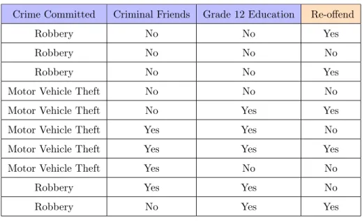
The raw data used in this example can be seen in Table 3.1. There are three features, “Crime Committed”, “Criminal Friends”, and “Grade 12 Education”, that correspond to different outcomes of the classification feature “Re-offended” (“Yes” and “No”).

For a set of features, X, the prediction value, Xmk, of the classification feature, Xm, for each class, k

(29)

Crime Committed Criminal Friends Grade 12 Education Re-offend

Robbery No No Yes

Robbery No No No

Robbery No No Yes

Motor Vehicle Theft No No No

Motor Vehicle Theft No Yes Yes

Motor Vehicle Theft Yes Yes No

Motor Vehicle Theft Yes Yes Yes

Motor Vehicle Theft Yes No No

Robbery Yes Yes No

Robbery No Yes Yes

Table 3.1: Re-offense Raw Data Table for Naive Bayesian Example

When there are multiple features,m1,m2, ...,m|X|, the equation for the prediction value is,

Xmk=argmaxxj∈XP(xj)

|X|

Y

i=1

P(mi|xj),

where |X| is the number of elements in the data set X. It is applied to all classifications, Xmk, and the

largest resulting value is the final classification, likely or not likely to re-offend. The P(mi|xj)is given by

P(mi|xj) =

nc+wp

n+w ,

where n is the number of data matching the desired classification value xj, nc is the number of data that

match both the desired classification value xj and the feature valuemi, pis the prior estimate of the value

ofP(mi|xj), andwis called the equivalent sample size1and adds a weighted respective of the observed data

to the valuep. For a deeper explanation of this formula see (Kubat,2015). In this example, the value ofwis

chosen to be 3 for all calculations because there are three features other than the classification feature in the data set, and thepvalue is0.5to reflect that the values of each feature in the data set are binary (Meisner, 2003).

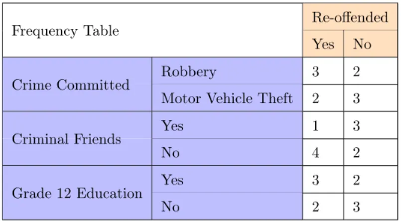
From the raw data in Table 3.1, a frequency table is calculated that details the number of times an instance has occurred when certain conditions are present; see Table 3.2. The Naive Bayesian classifier assumes the instances and conditions are independent of each other; this is the naive aspect of the classifier.

To give a full classification or prediction, theXmkvalue must be calculated for all classification outcomes

given the predictor, and the resulting outcome is the highest probability value. For this example, the goal is to determine if an individual is likely to re-offend or not when they have committed a robbery, have criminal friends, and do not have a grade 12 education.

1_{This value is also referred to as the m-estimate, not to be confused with the variable}_m_{that represents a feature in the}

(30)

Re-offended Frequency Table

Yes No

Robbery 3 2

Crime Committed

Motor Vehicle Theft 2 3

Yes 1 3 Criminal Friends No 4 2 Yes 3 2 Grade 12 Education No 2 3

Table 3.2: Frequency Table

The probability, P(mi|xj), for the outcome or class “Yes” and the attributes or predictors “Robbery”,

“Criminal FriendsY es”, and “Grade 12N o” is calculated in equation (3.1) using the values in the frequency

table. Lastly, the Xmk value is calculated using the calculated probabilities.

P(Robbery|Yes) =3 + 3∗0.5 5 + 3 = 0.56

P(Criminal FriendsY es|Yes) =

1 + 3∗0.5 5 + 3 = 0.31 P(Grade 12N o|Yes) = 2 + 3∗0.5 5 + 3 = 0.43 P(Robbery) = 5/10 = 0.5 P(c) =P(Yes) = 5/10 = 0.5

Xmk=P(Robbery|Yes)∗P(Criminal FriendsY es|Yes)∗P(Grade 12N o|Yes)∗P(Yes)

= 0.56∗0.31∗0.43∗0.5 = 0.037

(3.1)

The results for the firstXmk,P(Yes|Robbery), are calculated, the next value to be calculated determines

(31)

probability values to determine theXmk value for P(No|Robbery), P(Robbery|No) = 2 + 3∗.5 5 + 3 = 0.43 P(Criminal FriendsY es|No) = 3 + 3∗.5 5 + 3 = 0.56 P(Grade 12N o|No) = 2 + 3∗.5 5 + 3 = 0.56 P(c) =P(No) = 5/10 = 0.5

Xmk=P(Robbery|No)∗P(Criminal FriendsY es|No)∗P(Grade 12N o|No)∗P(No)

= 0.43∗0.56∗0.56∗0.5 = 0.069

(3.2)

The two results are then compared, and the higher value has the greater probability of happening, ultimately classifying the data as re-offending or not. The posterior probability for notre-offending is 0.069 and for re-offending after committing a robbery is 0.037. The posterior probability fornotre-offending after committing a robbery is greater; therefore the Naive Bayesian classifier classifies an individual as not likely to re-offend if they have committed a robbery, have criminal friends, and do not have a grade 12 education. This classification process is more complicated as the number of features in the data set increases, but it works well for large amounts of data.

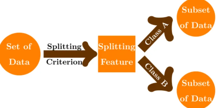
3.2 Decision Trees

DTs are a supervised machine learning method that classify data using a tree-like structure. DTs fall into the category of a supervised machine learning method because the training data used to build the model contain the classification feature (Marsland, 2015). DTs learn simple decision rules from the training data and structure these rules to form the tree-like model. The DT model can be used to classify new sets of data. Figure 3.1 is a visual representation of the DT method. A DT is a classifier that contains nodes that are directly connected to the root node at the top of the tree by edges. Each node with an outgoing edge is called a test node; these nodes represent features in the data set. Nodes with no outgoing edges are called leaves; these nodes give a classification result. After the tree is built, it can be used to classify outcomes from a given data set.

The Selective Decision Tree Classifier: A Novel Classifier based on Feature Selection