Questioni di Economia e Finanza
(Occasional Papers)
Pro-cyclicality of capital regulation: is it a problem? How to fix it?
by Paolo Angelini, Andrea Enria, Stefano Neri, Fabio Panetta and Mario Quagliariello
Number
74
Oct
ober 20
Questioni di Economia e Finanza
(Occasional papers)
Number 74 – October 2010
Pro-cyclicality of capital regulation: is it a problem? How to fix it?
The series Occasional Papers presents studies and documents on issues pertaining to the institutional tasks of the Bank of Italy and the Eurosystem. The Occasional Papers appear alongside the Working Papers series which are specifically aimed at providing original contributions to economic research.
The Occasional Papers include studies conducted within the Bank of Italy, sometimes in cooperation with the Eurosystem or other institutions. The views expressed in the studies are those of the authors and do not involve the responsibility of the institutions to which they belong.
PRO-CYCLICALITY OF CAPITAL REGULATION: IS IT A PROBLEM? HOW TO FIX IT
?
by Paolo Angelini*, Andrea Enria**, Stefano Neri*, Fabio Panetta* and Mario Quagliariello**
Abstract
We use a macroeconomic euro area model with a bank sector to study the pro-cyclical effect of the capital regulation, focusing on the extra pro-cyclicality induced by Basel II over Basel I. Our results suggest that this incremental effect is modest. We also find that regulators could offset the extra pro-cyclicality by a countercyclical capital-requirements policy. Our results also suggest that banks may have incentives to accumulate countercyclical capital buffers, making this policy less relevant, but this finding is depends on the type of economic shock posited. We also survey different policy options for dealing with procyclicality and discuss the pros and cons of the measures available.
JEL Classification: E32, E44, E58. Keywords: Basel accord, pro-cyclicality.
________________________
*
Banca d’Italia, Economic Outlook and Monetary Policy Department.
**
Contents
1. Introduction ... 7
2. The macro framework ... 9
2.1 Main features of the model... 10
2.2 Key changes to the analytical framework ... 11
3. The pro-cyclicality of the Basel II framework: Is it a problem?... 13
3.1 Baseline results... 14
3.2 Robustness ... 18
3.3 Summary ... 19
4. Assessing costs and benefits of countercyclical measures... 20
4.1 Instituting a countercyclical capital requirement ... 20
4.1.1 Countercyclical management of capital requirements ... 21
4.1.2 Would banks voluntarily adopt a countercyclical capital policy rule? ... 24
4.2 Increasing banks’ regulatory capital ... 25
5. Technical Discussion ... 30
6. The policy debate on countercyclical tools ... 31
6.1 Review of the main proposals... 31
6.1.1 Smoothing the inputs of the capital function... 31
6.1.2 Strengthening stress tests... 31
6.1.3 Adjusting the capital function ... 32
6.1.4 Smoothing the output of the capital function ... 32
6.1.5 Buffers based on risk-sensitive conditioning variables... 33
6.1.6 Countercyclical provisioning... 33
6.2 Critical assessment of the proposals ... 34
6.3 The proposals of the Basel Committee ... 36
7. Conclusions ... 37
References ... 40
7
1. Introduction1
Since the end of the 1980s, following the implementation of the Basel rules, G10 countries have introduced bank capital requirements based on risk-weighted assets. At the microeconomic level, the reasons for capital regulation include potentially excessive
risk-taking by bank managers induced by flat-premium deposit insurance schemes2 and
insufficient monitoring of lending policies by small, dispersed depositors.3 From a
macroeconomic perspective, risk-based capital requirements are one of the tools available for reducing the externalities associated with bank failures (in terms, for example, of public funds
needed in case of systemic crises or contagion across intermediaries).4
While there is strong rationale for their adoption, a potential drawback of risk-based capital requirements is that they could amplify the cyclical fluctuations of the economy (i.e. they may generate pro-cyclicality). In theory, in a frictionless economy they should not, but imperfections in capital markets do exist, and an accelerator mechanism may generate feedback from bank capital to the real economy (Adrian and Shin 2008). Therefore, risk-based capital requirements could generate pro-cyclicality, because risk itself is cyclical both
in quantity and in value.5 The debate on the additional pro-cyclicality generated by capital
regulation, however, is still open. To conclude that capital regulation has pro-cyclical effects one should check, first of all, that it induces cyclicality in the minimum regulatory capital requirement under Pillar I, and that such cyclicality survives the supervisory review process under Pillar II (in principle, the regulator could take steps to attenuate it). Second, it should be ascertained that the banks’ response to the regulatory changes does not offset the additional pro-cyclicality (e.g. via voluntary accumulation of countercyclical capital buffers). Finally,
one should check that any resulting additional cyclicality in bank lending affects real activity.6
Although our knowledge about each of these conditions is very limited, in the aftermath of the current financial crisis a consensus has emerged that the Basel II capital rules should be amended. Widely discussed proposals, to be implemented once the crisis is over and phased in gradually, would focus on the level and the dynamics of bank capital. They include: strengthening the capital base of banks; implementing mechanisms for building capital buffers and forward-looking provisions in periods of buoyant growth for use in downturns;
1 The views expressed in the paper do not necessarily reflect those of the Bank of Italy. We wish to thank F.
Saccomanni for providing us with the incentive to work on the paper, as well as K. Regling and H. H. Kotz (our discussants at the Conference “An Ocean Apart? Comparing Transatlantic Responses to the Financial Crisis” jointly organized by Banca d’Italia, Bruegel and PII.E. with the support of the European Commission and held in Rome, 10-11 September 2009), E. Gaiotti and A. Gerali for useful comments on a previous draft. All remaining errors are our own.
2 See Kohen and Santomero (1980), Kim and Santomero (1988), Rochet (1992). 3 See Dewatripont and Tirole (1994).
4 See Kashyap and Stein (2004).
5 The amount of risk tends to increase during contractions, partly reflecting the process of accumulation
during expansions (Borio et al. 2001). Similarly, the price of risk – that is, investors’ risk aversion – decreases during upswings and increases during downswings (Lowe 2002).
6 These conditions have been pointed out by a number of authors. See Taylor and Goodhart (2004) for
8
harmonising the definition of eligible capital and improving its quality; complementing Basel II rules with non-risk-based limits to leverage; introducing liquidity requirements (G20, 2009; FSF, 2009). The challenge is not reaching an agreement on general principles, but translating principles into concrete measures, which can be applied consistently across jurisdictions. The current state of the debate prompts a series of considerations. First, the above-mentioned proposals for reform are generally analysed on a piecemeal basis, in the absence of a consistent framework that would allow a more structured approach to capital regulation. Moreover, the proposals pursue the twofold objective of increasing the resilience of the financial system and mitigating the pro-cyclical effects of capital regulation, at times without clearly distinguishing between the two. Finally, in our view, the recent contributions by regulators (Basel Committee 2010b, Macroeconomic Assessment Group 2010) and by the private sector (Institute of International Finance 2010) on the macroeconomic impact of the regulatory reform can be enriched with further cost-benefit analyses.
Moving from these considerations, this paper seeks to deal with these issues in a systematic way. We believe that a comprehensive framework should address the following fundamental questions: (i) Does the new Basel II regime really increase the pro-cyclicality of the banking system, and if so, by how much? (ii) Higher capital requirements would clearly strengthen the resilience of the financial system; could they also help attenuate the cyclical effects of credit on GDP, consumption and investment? (iii) What room is there for the management of countercyclical capital requirements? (iv) What is the macroeconomic cost (e.g. in terms of
GDP growth) of policies to attenuate pro-cyclicality?7
To address these questions we cast the regulator problem within a macroeconomic model. Specifically, we build on the DSGE model developed by Gerali et al. (2009) to examine the functioning and possible shortcomings of risk-based capital regulation and potential policy measures designed to mitigate pro-cyclicality. The model features a simplified banking sector with capital, capturing the basic elements of banks’ balance sheets: on the assets side there are loans to firms and households; on the liabilities side, deposits held by households and capital. We support this model by introducing heterogeneity in the creditworthiness of the various economic operators. We also introduce risk-sensitive capital requirements and quantify the extent to which they induce excessive lending and excessive GDP growth in booms, the reverse in downturns. We assess the effectiveness of stylised countercyclical tools on the basis of the model. In particular, we look at the response of the key macroeconomic variables to higher capital requirements and to passive and active countercyclical capital policies. A final section is devoted to the practical aspects of the implementation of countercyclical capital rules. In particular, we focus on two tools: (i) the accumulation of Basel II capital buffers calibrated on downturn conditions (e.g. adopting simple correction factors based, for instance, on the ratio between downturn and current PDs); (ii) dynamic provisioning based on through-the-cycle expected losses. We argue that these tools may complement each other and are an essential element in any countercyclical toolkit.
The paper makes two main contributions to the literature. First, it studies the role of capital regulation in the context of a macroeconomic model, which allows us to examine the general
7 A fifth crucial issue, which we do not address here, concerns the systemic nature of certain risks: risk-based
capital regulation that only refers to individual banks underestimates systemic risk by neglecting the macro impact of banks reacting in unison to a shock (Brunnermeier et al. 2009).
9
equilibrium effects of changes in bank capital regulation. The DSGE model used in the paper belongs to a new class that explicitly comprises a (simplified) financial sector and features a meaningful interaction between this sector and the real economy. However, a caveat is needed. Our model is still far too simplified to be able to capture a number of essential elements of the financial sector, some of which arguably played an important role during the current financial crisis – e.g., maturity mismatches, derivative products, liquidity issues, heterogeneity across financial institutions. Regarding these clear weaknesses, it is worth recalling that the financial sector was entirely absent in the DSGE models of the previous generation. The financial accelerator mechanism of Bernanke, Gertler and Gilchrist (1999) has only recently been reconsidered in standard medium-scale DSGE models. One possible reason why the empirical literature, in particular, has generally not considered this mechanism is that it does not significantly amplify the effects of monetary policy shocks.
Second, we supplement this simplified but rigorous framework with a discussion of the main policy proposals. This approach stands in sharp contrast both with the existing literature on financial stability issues, typically based on reduced-form, partial-equilibrium models, and with the theoretical macroeconomic literature, typically not concerned with the practical implementation of policy proposals. We are aware of only one paper that studies the additional pro-cyclicality introduced by Basel II relative to Basel I in a similar macroeconomic framework: Aguiar and Drumond (2009). They find that the amplification of monetary policy shocks induced by capital requirement becomes stronger under Basel II regulation.
2. The macro framework
Until recently, the financial sector was largely overlooked in macroeconomic modeling. Seminal contributions, starting from Bernanke, Gertler and Gilchrist (1999), have begun to fill the gap by introducing credit and collateral requirements in quantitative general equilibrium models. More recently, models have begun to be designed to study the role of financial intermediaries in general and banks in particular (Christiano, Motto and Rostagno 2007, and Goodfriend and McCallum 2007). These models, however, mainly emphasise the demand side of credit. The credit spread that arises in equilibrium (called the external finance premium) is a function of the riskiness of entrepreneurs’ investment projects and/or their net wealth. Banks, operating under perfect competition, simply accommodate the changing conditions from the demand side.
Gerali et al. (2009) instead build on the idea that conditions from the supply side of the credit markets are key to shape business-cycle dynamics. Starting from a standard model, featuring credit frictions and borrowing constraints as in Iacoviello (2005) and a set of real and nominal frictions as in Christiano et al. (2005) or Smets and Wouters (2003), they add a stylised banking sector with three distinctive features. First, banks enjoy some degree of market power when setting rates on loans to households and firms. Second, the rates chosen by these monopolistically competitive banks are adjusted only infrequently – i.e. they are sticky. Third, banks accumulate capital (out of retained earnings), as they try to maintain their capital/assets ratio as close as possible to an (exogenously given) optimal level. This optimal level might derive from a mandatory capital requirement (like those explicitly set forth in the Basel accords). In a deeper structural model, the optimum level might relate to the equilibrium outcome from balancing the cost of funding with the benefits of having more ‘skin in the
10
game’ to mitigate typical agency problems in credit markets. The model is estimated with Bayesian techniques using data for the euro area from 1998 to 2009.
Banks make optimal decisions subject to a balance-sheet identity, which forces assets (loans) to be equal to deposits plus capital. Hence, factors that affect the impact of banks’ capital on the capital/assets ratio force banks to modify their leverage. Thus, the model captures the basic mechanism described by Adrian and Shin (2008), which has arguably played a major role during the current crisis.
In this paper we modify the model by Gerali et al. (2009) to study the role of capital regulation. More specifically, we assume that credit risk differs across categories of borrowers and introduce risk-sensitive capital requirements. We then show how optimal lending decisions of banks, and hence the macro environment, are affected by different regulations. We refer readers to the original paper for a more thorough description of the basic features of the model.
2.1 Main features of the model
The model describes an economy populated by entrepreneurs, households and banks. Households consume, work and accumulate housing wealth, while entrepreneurs produce goods for consumption and investment using capital bought from capital-good producers and labour supplied by households.
There are two types of households, which differ in their degree of impatience, i.e. in the discount factor they apply to the stream of future utility. This heterogeneity gives rise to borrowing and lending in equilibrium. Two types of one-period financial instruments, supplied by banks, are available to agents: saving assets (deposits) and loans. Borrowers face a collateral constraint that is tied to the value of collateral holdings: the stock of housing for households and physical capital for entrepreneurs.
As mentioned above, the banking sector operates in a regime of monopolistic competition: banks set interest rates on deposits and on loans in order to maximise profits. The balance sheet is simplified but captures the basic elements of banks’ activity. On the assets side are loans to firms and households. On the liabilities side are deposits held by households and capital. Banks face a quadratic cost of deviating from an ‘optimal’ capital to assets ratio .8
(1) bt t t b b L K K , 2 ,
where Kb,t is bank capital, Lt is total loans and b is a parameter measuring the cost of
deviating from . The lattercan be thought of as a minimum capital ratio established by the
8 The adjustment cost adopted in equation 1 is quadratic, and hence symmetric. An alternative, more realistic
version should be asymmetric – the cost of falling below a regulatory minimum is arguably higher than the cost of excess capital. However, the first-order approximation of the model which we use throughout the current version of the paper would make such alternative adjustment cost immaterial for the results. In future work we plan to introduce an asymmetric adjustment cost (see Fahr and Smets 2008 for an application of downward nominal wage rigidities) and look at a second order approximation of the model, or simulate the nonlinear model.
11
regulator, plus a discretionary buffer. When the capital ratio falls below , cost increases are
transferred by banks onto loan rates:
(2) t t t b t t b b t i t markup L K L K R R 2 , , , i=H, F
where Rt is the monetary policy rate and markup captures the effects of monopolistic power of
banks on interest rate setting.9 Equation 2 highlights the role of bank capital in determining
loan supply conditions. On the one hand the bank would like to extend as many loans as possible, increasing leverage and thus profits per unit of capital. On the other hand, when
leverage increases, the capital/assets ratio falls below and banks pay a cost, which they
transfer on the interest rates paid by borrowers. This, in turn, may reduce credit demand and hence bank profits. The optimal choice for banks is to choose a level of loans (and thus of leverage) such that the marginal cost of reducing the capital/assets ratio exactly equals the
spread between i
t
R and Rt . The presence of stickiness in bank rates implies that the costs
related to the bank capital position are transferred gradually to the interest rate on loans to
households and firms. Bank capital is accumulated out of retained profits π, according to the
following equation:
(3) Kb,t
1b
Kb,t1b,t1where the term bKb,t1 measures the cost associated with managing bank capital and
conducting the overall intermediation business.
Monetary policy is modelled via a Taylor rule with the following specification: (4) Rt
1R
R
1R
t
y
yt yt1
RRt1The values of the parameters of the model are reported in Gerali et al. (2009).
2.2 Key changes to the analytical framework
We have made a few changes to the basic framework of Gerali et al. (2009) in order to adapt it to our purposes. Specifically, we assume that loans to firms and to households are
characterised by different degrees of riskiness captured, in a reduced form, by weights, F
t
w and
H t
w , which we use to compute a measure of risk-weighted assets.10 The capital adjustment
cost (1) is modified as follows:
9 In practice, a dynamic version of equation 2, in which bank rates are sticky, is employed in the model (see
Gerali et al. 2009). It is assumed that banks, at any point in time, can obtain financing from a lending facility at the central bank at a rate equal to the policy rate Rt. A no-arbitrage condition between borrowing from the
central bank and from households by issuing deposits implies that in equilibrium a dynamic version of equation 2 must hold.
10 The model does not contemplate defaults, as they are ruled out as equilibrium outcomes (see Kyiotaki and
Moore, 1997, and Iacoviello, 2005), but the device we adopt does mimic the effect of capital requirements based on risk-weighted assets.
12 (5) H bt t H t F t F t t b b v K L w L w K , 2 , ,
where total loans Lt is replaced by the sum of risk-weighted loans to firms ( F
t
L ) and
households ( H
t
L ).
Note that setting F
t
w = H
t
w =1 in expression 5 simulates the Basel I regime for loans to the
private sector, whereas allowing the weights to vary over time captures the essence of the risk-sensitive Basel II mechanism. Under it, the inputs of the capital function can change through the cycle, reflecting either the rating issued by rating agencies or banks’ own internal risk assessment models (the IRB approach). Under this second interpretation, we model the weights so as to roughly mimic their real-world setting by banks. We assume simple laws of motion of the form:
(6)
i t i t t i i i i i t w Y Y w w 1 1 log log 4 1 i= F, Hwhere the lagged term i
t
w1 models the inertia in the adjustment of the risk-weights and the
parameteri (<0) measures the sensitivity of the weights to cyclical conditions proxied by the
year-on-year growth rate of output.11
It is important to note that appropriate choices for the parameters in equation 6 also allow us to study the system dynamics under the two main rating systems allowed by the regulation: ‘point in time’ (PIT) v. ‘through the cycle’ (TTC). Essentially, to assess borrowers’ creditworthiness under Basel II, banks can either use ratings supplied by external rating agencies, or produce their own internal ratings. Regardless of the source, ratings can be attained via either a PIT or a TTC approach. PIT ratings represent an assessment of the borrower’s ability to discharge his obligations over a relatively short horizon (e.g. a year), and so can vary considerably over the cycle. The TTC approach focuses on a longer horizon, abstracting in principle from current cyclical conditions. TTC ratings are therefore inherently
more stable than PIT ratings, although their predictive power for default rates is lower.12
Within our framework, the TTC approach could be approximated by choosing a large value
for ρ and a small one for in (6). At the limit, in this simplified setting a pure TTC system
coincides with the Basel I framework.
Summing up, the results in the following sections can be interpreted as a comparison between the Basel I and Basel II frameworks, but also as a comparison between the PIT and the TTC approaches within the Basel II framework. While for the sake of brevity our comments refer mainly to the first interpretation, the second should also be kept in mind.
A final remark concerns the interpretation of , the ‘optimal’ capital/assets ratio appearing in
equations 2 and 5. As mentioned above, can be thought of as a minimum capital ratio
established by the regulator – e.g. the 8 percent benchmark imposed by the Basel regulation, plus a buffer. The buffer captures the idea that banks tend to voluntarily keep their capital
11 The results illustrated below remain broadly unchanged if the business cycle is measured using the deviation
of output from its steady-state level.
13
above the regulatory minimum, to avoid extra costs related to market discipline and
supervisory intervention, or to meet market expectations (e.g. to maintain a given rating).13
This twofold interpretation of , as a regulatory instrument and as a capital buffer held by
banks, has a key role in the present paper and must be borne in mind for the interpretation of our results. We shall come back to it in the following sections.
3. The pro-cyclicality of the Basel II framework: Is it a problem?
Whereas there is a relatively broad consensus that Basel I – like any capital regulation – increased the cyclicality of the financial system, the issue of how much additional
pro-cyclicality Basel II generates relative to Basel I is still open.14 This issue is hard to address
empirically, in view of the extremely recent application of Basel II (in Europe most banks deferred it to 2008). What scanty evidence there is derives from counterfactual and simulation exercises, or from comparisons with similar past experiences of regulatory change. Many authors argue that this extra pro-cyclicality may be substantial. However, the result often depends on the credit-risk estimation techniques chosen. In addition, other authors observe that banks hold capital buffers in excess of the regulatory minimum, and that this could enable
them to smooth or even eliminate the impact of the new regulation on lending patterns.15
Overall, a tentative summary of the available literature is that Basel II may increase the pro-cyclicality of bank lending, but that this conclusion must be treated with caution. Furthermore, as we argued in the introduction, little if any evidence is yet available on the impact of the new regulation on the real economy – i.e. on GDP and its components, and lending – which is what ultimately matters to assess pro-cyclicality.
This section develops that analysis. Specifically, we use the model augmented with the estimated versions of (6) to compare the model dynamics under Basel I and Basel II, and assess whether Basel II induces extra swings in bank variables and the key macro variables, and the size of these swings. To this end, we compute impulse-response functions to various shocks. We focus on technology shocks, which are arguably the main drivers of the business cycle, but we also consider monetary policy and demand shocks.
We use the parameterisation of the model reported in Gerali et al. (2009). To make the model operational we need to estimate the parameters of (6). Taking this equation to the data presents several challenges, due to the fact that no historical time series for the weights or the risk-weighted assets is available yet. To obtain estimates of the parameters of (6) we proceed as follows. We use data on delinquency rates on loans to households and non-financial companies in the US as proxies for the probabilities of default on these loans (similar data for the euro area were not available to us). We input these time series into the Basel II capital requirements formula, and using a series of assumptions concerning the other key variables of
13 See Furfine (2001).
14 The Basel Committee was well aware of the potential pro-cyclical effects of the new regulations. The
‘through the cycle’ philosophy that permeates the accord, and several explicit provisions therein, were meant to curb pro-cyclicality. However, the evidence suggests that the implementation did not fully conform to the regulation’s spirit. See Cannata and Quagliariello (2009).
15 See Panetta et al. (2009) and Drumond (2008) for reviews of the literature on the pro-cyclicality of capital
14
the formula (loss given default, firms’ size, loan maturity) we are able to back out time series
for the weights F
t
w , H
t
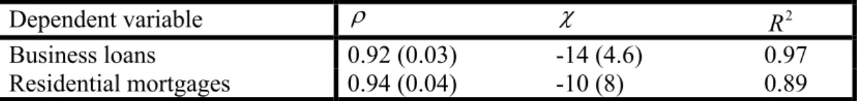
w . Next, we estimate equation 6 using these series. The regressions
suggest that the sensitivity of the risk weights to the cycle (the parameter χ) is relatively
strong for commercial and industrial enterprises but not statistically different from zero for residential mortgages. Details on the methodology used to obtain the weights are reported in the Appendix 1.
3.1 Baseline results
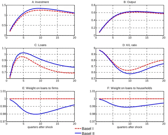
Figure 1 shows the results for the technology shock, modelled as an unexpected increase in total factor productivity (TFP). Consider first the results under Basel I (represented in the figure by the dashed red lines).
The top two panels report the response of the key macroeconomic variables. The main effect works through investment: firms react to the positive technology shock by increasing investment by about 1 percent above its steady-state level in the first year (panel A). The expansion of output is relatively more muted and delayed (panel B), reflecting a more gradual pick-up in consumption. The increase in investment drives up the demand for loans, so that one year after the shock loan growth is about 0.9-1.0 percent above steady state (panel C). Figure 1 - Impulse responses to a positive technology shock: Basel I v. Basel II
0 5 10 15 20 0 0.5 1 1.5 A: Investment 0 5 10 15 20 0 0.2 0.4 0.6 0.8 B: Output 0 5 10 15 20 0.7 0.8 0.9 1 1.1 C: Loans Basel I Basel II 0 5 10 15 20 8.5 8.6 8.7 8.8 8.9 9 D: K/L ratio 0 5 10 15 20 0.97 0.98 0.99 1 1.01
E: Weight on loans to firms
quarters after shock
0 5 10 15 20 0.97 0.98 0.99 1 1.01
F: Weight on loans to households
quarters after shock
Note: The impulse responses are measured as percentage deviations from steady state, except for the K/L ratio (measured in percentage points) and the weights wi (normalised to 1 and measured in levels).
15
The ratio between bank capital and assets declines over the first two or three years. The minimum value, close to 0.4 percentage points below the 9 percent steady-state value, is reached after 10 quarters (panel D). The decline reflects the increase in loans in the denominator (panel C), as well as a contraction of bank profits, which affects the numerator via the bank capital accumulation equation (3). The decline in profits is related to the decrease in the policy rate by the central bank in response to the decline in inflation, and to the presence of a mark-up on the loan rates and a mark-down on deposit rates. The mark-up and the mark-down are sticky. Hence, as the policy rate is reduced by the central bank, the interest
rate margin falls and, since the price effect dominates the quantity effect, so do profits.16
Notice that by construction the weights i
t
w in panels E and F do not move, as under Basel I
they are fixed at 1.
Consider next the same exercise under Basel II (represented by the solid blue lines). In a nutshell, the system’s responses are qualitatively similar, but slightly more pronounced than
in the Basel I scenario. The reduction in the risk weights i
t
w is the key driver of the system’s
enhanced response. Both weights decline in the two years after the shock, reflecting improved macroeconomic conditions and the related decrease in the riskiness of the loans. The sharper
decline of F
t
w is due to its higher sensitivity to cyclical conditions (a higher i in (6)). This
drives the ratio between banks’ capital and risk-weighted assets away from the desired value
. To boost loans and reduce this gap, banks reduce interest rates on loans more aggressively
than under Basel I.
The response of bank credit is always above the corresponding curve under the Basel I framework. The effect is relatively small, however. A similar reaction emerges for banks’
capital/assets ratio.17 The expansion in bank credit boosts investment growth: the deviation
from steady state peaks about two years after the shock, at about 1.4 percent, compared with about 1.3 under Basel I. The effect on output is also magnified but muted.
Figure 2 shows the results for an expansionary monetary policy shock. The effects on the macroeconomic variables are qualitatively analogous to those in Figure 1: in the first 8-10 quarters the curves for Basel I are systematically below those for Basel II. However, the difference is negligible, as the curves virtually overlap. The limited impact of Basel II reflects
the behaviour of the time-varying weights i
t
w: whereas the technology shock described in
Figure 1 induces a large and persistent decline in the weights, the monetary policy shock causes a reduction of the risk weights that is too small and short-lived to alter the dynamics of the bank and macro variables significantly. In turn, this is due to the small and short-lived reaction of output to a monetary policy shock (a relatively common finding in the DSGE literature). The small additional pro-cyclicality induced by Basel II according to the exercises in Figure 2 echoes several findings in the literature, according to which financial frictions do not significantly amplify the transmission of monetary policy shocks (see, among others, De Fiore and Tristani 2009, De Graeve 2008 and Iacoviello 2005). At the same time, our result is in contrast with Aguiar and Drumond (2009), the only other paper which focuses on the Basel I v Basel II issue within a DSGE framework. They find that, in the case of a monetary policy shock, the impact of Basel on the model dynamics in general and on output in particular is
16 Empirically, the differential between loan and deposit rates is countercyclical. See e.g. Aliaga-Diaz and
Olivero (2008) for evidence on the US.
16
larger than in our case (both for the effect of Basel I, and for the Basel II v. Basel I differential).18
As a third experiment, we examined a positive demand shock, modelled as a decrease in the intertemporal discount factor that induces both types of household to anticipate consumption and reduce savings. This type of disturbance, which directly affects households’ inter-temporal first-order conditions, is commonly considered in estimated medium-scale models (see Primiceri et al. 2006 and Smets and Wouters, 2007). One of its characteristics, in these models, is that it typically generates opposing movements in consumption and investment. This does not match the pattern observed in reality, as in most economies the correlation, along the business cycle, between consumption and investment is strongly positive. Thus, the quantitative importance of these shocks for the business cycle tends to be relatively modest, and the positive correlation between consumption and investment may reflect other, more important drivers of the business cycle (e.g. technology shocks, which push consumption and investment in the same direction).
Figure 2 - Impulse responses to a positive monetary policy shock: Basel I v Basel II
0 5 10 15 20 -0.2 0 0.2 0.4 0.6 A: Investment 0 5 10 15 20 -0.05 0 0.05 0.1 0.15 B: Output 0 5 10 15 20 -0.2 0 0.2 0.4 0.6 C: Loans Basel I Basel II 0 5 10 15 20 8.9 8.95 9 9.05 9.1 D: K/L ratio 0 5 10 15 20 0.97 0.98 0.99 1 1.01
E: Weight on loans to firms
quarters after shock
0 5 10 15 20 0.97 0.98 0.99 1 1.01
F: Weight on loans to households
quarters after shock
Note: the impulse responses are measured as percentage deviations from steady state, except for the K/L
(measured in percentage points) and the weights wi (normalised to 1 and measured in levels).
18 This difference may be due to alternative modeling choices. Aguiar and Drumond (2009) build on the
Bernanke, Gertler and Gilchrist (1999) framework, whereas our model is based on the financial accelerator mechanism of Kyiotaki and Moore (1997).
17
The debate on this issue is clearly beyond the scope of this paper. For our purposes, it is important to remark that following this type of demand shock investment falls, and so does bank lending; these movements are attenuated (i.e. the contraction is more modest) under Basel II. Overall, output growth is (slightly) stronger under Basel II, as the growth in
consumption offsets the fall in investment.19 Thus, using the strict GDP-based interpretation
of the definition of cyclicality proposed in the introduction (an arrangement is pro-cyclical if it amplifies the pro-cyclical fluctuations of the economy), we can still conclude that adoption of Basel II produces a (modest) increase in pro-cyclicality. However, the muted contraction of bank loans (and investment) under Basel II makes one wonder whether simply looking at the behaviour of output is the proper thing to do.
Summing up, our findings suggest that the transition from Basel I to Basel II can amplify the dynamics of bank lending and of the capital/asset ratio and, ultimately, the fluctuations of the real economy. Furthermore, recalling that our exercises in Figures 1 and 2 can also be interpreted as a comparison between the PIT and TTC rating approaches under Basel II, our evidence also suggests that the PIT approach introduces extra pro-cyclicality relative to the TTC. Our key finding, however, is that the magnitude of this amplification effect is relatively small.20
This assessment has to be qualified with two caveats. First, there are at least two reasons why, ceteris paribus, the above exercises may overestimate Basel II’s incremental pro-cyclicality. One is that they only partially incorporate banks’ optimal response to shocks and regulatory changes. As we discuss below, several authors contend that forward-looking banks will react to Basel II by holding voluntary countercyclical buffers. By contrast, we have assumed so far
that (the parameter pinning down the steady-state value of banks’ capital/assets ratio) does
not vary over time. We shall address the issue of a time-varying in section 5.1. Another
potential source of overestimation is that our estimates of equation 6 are based on quarterly delinquency rates, and should therefore approximate a pure PIT approach.
Second, several shortcomings of the model may have an ambiguous impact on the magnitude of the effect we are investigating, thereby increasing the confidence interval around our assessment. Other features not yet discussed are likely to generate an underestimation of this effect. We discuss them in section 5.
19 The decrease in households’ discount factor makes them more impatient and causes an increase in
consumption and output, and a reduction in savings (deposits fall by around 0.6 percent). The fall in deposits forces banks to reduce lending to firms (who cut investment spending) and to households. The initial increase in spending on capital goods reflects the large increase in the price of firms’ installed capital stock. The fall in risk-weighted loans and the slow increase in bank capital, resulting from higher profits, raises the capital/asset ratio above the desired value . As for the technology shock, both weights decline in response to the demand shock. Profits increase under Basel I but fall under Basel II. This difference reflects the response of loan rates, which increase more under Basel I than under Basel II.
20 Our assessment of the pro-cyclicality of capital regulation may be affected by the parameter measuring the
18 3.2 Robustness
Our results are sensitive, inter alia, to the estimated values of and , whose point estimates are subjected to particular uncertainty, for the reasons just mentioned. Therefore, we now assess the sensitivity of our findings to alternative values for ρi and i, the key parameters in equation 6. We gauge the impact of modifying these parameters on output and bank loans, the key variables that characterise the results of Figures 1 and 2. We replicate the exercise
underlying the figures under different values of ρi and i. These figures are judgmental – i.e.
they are not estimated – and their only aim is to test the robustness of our results. In Table 1 we only report the results for the technology shock, as those for the monetary policy shock remain virtually unchanged.
For ease of comparison, the intersections of the rows and columns labelled ‘baseline’ report results from Figure 1, Basel II scenario. For instance, consider the effect of the technology
shock on output (left-hand side of the table). Using the baseline estimates of i and i one
obtains a maximum deviation of investment from its steady-state value of 0.6 percent. This value is the maximum of the impulse-response curve of output under the Basel II regime, reached after about 7 or 8 quarters (Figure 1.B). Likewise, the maximum effect on loans, 1 percent of the steady-state value, reached after 5 quarters, can be read from Figure 1.C.
Table 1 - Sensitivity of results to parameterisation of equation (6): technology shock
(Maximum effect;percentdeviations from steady state) Effect on output (0.6 under Basel I) Effect on loans (1.0 under Basel I) i i 0.70 Baseline 0.97 0.70 Baseline 0.97 Baseline 0.6 0.6 0.6 1.1 1.0 1.0 i Baseline * 5 0.7 0.7 0.7 1.9 1.4 1.1 Baseline* 10 0.8 0.9 0.7 3.1 2.4 1.5
Note: The baseline values for i and i (i=F, H) are those reported in the appendix, and used in Figures 1 and 2.
The estimated is in the range 0.90-0.93 (that is, it is greater than 0.7 and less than 0.97) for both households and firms.
The other cells of the table report the results of three exercises. First, we keep the
autoregressive parameters i fixed at their estimated baseline levels, and increase the
sensitivity i of the weights to the business cycle. Second, we move the autoregressive
parameters i above or below their estimated baseline levels while keeping the i at their
baseline values. Finally, we allow both parameters to differ from the baseline. Note that the
low-i, high-i cells can also be interpreted as corresponding to a version of the PIT rating
approach more extreme than that under our Basel II baseline scenario in Figures 1 and 2. By
contrast, the high-i, low-i cells could be viewed as capturing a TTC less extreme than under
our Basel I scenario in Figures 1 and 2.
Overall, this robustness check confirms the results of Figures 1 and 2. Consider first the effect on output (left-hand side of the table). In all cases the introduction of Basel II increases the pro-cyclicality relative to Basel I. Pro-cyclicality is also increased when moving from less to more PIT rating systems, i.e. moving from the upper-right to the lower-left corner of the table
19
(although a slight non-monotonicity appears in the figures: the effect under i=0.7 is slightly
larger than under the baseline value, which is above 0.9). The magnitude of the effects
induced by the Basel II regulation is almost insensitive to the autoregressive parameter i,
relatively more sensitive to the H, F parameters: assuming that the true values of these
parameters are 10 times larger than the estimated baseline, the pro-cyclical effect on output increases from 0.6 to 0.9 in terms of maximum deviation from the steady-state value. Overall,
the effects would remain modest even if we were to admit that our baseline i was
significantly underestimated.
Next, look at the effect on lending, on the right-hand side of the table. The above effects are
confirmed from a qualitative viewpoint, but become more sensitive to the choice of i and i.
In reaction to the technology shock, lending increases to a maximum of 2.3 percent of the
steady-state value when i are 10 times larger than the estimated baseline, compared with 1
percent when the baseline values are used.
We also check the sensitivity of the results to the estimated value of b, the parameter
measuring the cost of deviating from the optimal capital/assets ratio in (1). To this end, we
increase this parameter up to 10 times its baseline value, and compute the impulse responses for technology, monetary policy and demand shocks. These simulations reveal that the effect of this parameter is relatively large in the Basel I scenario (following a technology shock, the
expansion of loans and investment is smaller if b is larger); however, the difference between
Basel II and Basel I is only marginal.
3.3 Summary
In this section we have shown that the shift from Basel I to Basel II increases the pro-cyclicality of bank lending – i.e. that the reaction of macroeconomic variables such as output and investment to shocks is relatively larger under the Basel II than the Basel I regime. However, our results indicate that the magnitude of this amplification effect depends on the type of shock considered, and appears contained.
This conclusion is subject to a series of caveats. To begin with, the magnitude depends on a number of model features (discussed in section 5), which make our estimate particularly uncertain at this stage. In addition, admitting that the extra pro-cyclicality induced by Basel II is small does not imply that nothing should be done about it: if the cost of eliminating it were likewise small, then it would be optimal to address the problem. Finally, Aguiar and Drumond (2009), who employ a similar DSGE framework to address the issue, find that the amplification effect induced by Basel II is larger than suggested by our estimates.
Therefore, in the rest of the paper we consider possible remedies to the pro-cyclicality induced by the Basel II regulation, assessing their costs and benefits.
20
4. Assessing costs and benefits of countercyclical measures
A number of policy proposals to reduce the pro-cyclicality induced by Basel II have been advanced. Section 6 reviews and discusses these proposals in some detail. In short, they can
be grouped under the following headings: (i) smoothing the inputs of the capital function (for
instance, banks could be required to mitigate the cyclicality of their PIT estimates of the PDs,
or to go over to TTC estimation methods); (ii) adjusting the capital function (for instance,
some parameters such as the confidence level or the asset correlations could be appropriately
changed over the cycle); (iii) smoothing the output of the capital function (i.e. allow capital
requirements to move in an autoregressive or countercyclical fashion); (iv) adopting
countercyclical capital buffers; (v) adopting countercyclical provisions.
For the purposes of this section, it is enough to remark that the model with which we work does not allow us to distinguish among these proposals (as it makes no distinction between capital and loss provisions, say). However, it does allow us to assess their macroeconomic effects if one is willing to overlook the (important) technical differences among them, and concentrate instead on their common denominator. In our view, the common denominator is the idea that capital (or provisions) should be adjusted in a countercyclical fashion.
In the next subsection we gauge the effects on pro-cyclicality of countercyclical (regulatory or voluntary) capital buffers. In section 4.2 we assess the impact of higher capital requirements.
4.1 Instituting a countercyclical capital requirement
So far, we have worked under the assumption that the key parameter is time-invariant. This
is in keeping with the current policy framework, under both Basel I and II, and with the idea that banks like to keep voluntary capital buffers constant at the lowest possible value.
However, a natural extension is to consider a time-varying . Within our framework, this
represents the most straightforward way to assess the effect of countercyclical capital requirements. Consider the following equation:
(7) t
1
1
logyt logyt4
t1where the parameter measures the steady-state level of . In (7), we assume that t adjusts
to year-on-year output growth, our measure of the business cycle, with a sensitivity equal to
the parameter . Assuming that the latter is positive amounts to imposing a countercyclical
regulatory policy: capital requirements increase in good times (banks hold more capital for the amount of loans they provide to the economy), and decrease in bad times.
Note that adding (7) to the model affects the cyclical pattern of the main variables but not their steady-state levels, and is therefore neutral in this sense. The reason is that the steady
state of the model is affected only by the value of and not by the dynamics of , which are
influenced by the sensitivity of capital requirements to output. Therefore, in what follows we focus on the effects of adopting (7) on the dynamics of the economy.
21
Recall from section 2 that has a twofold interpretation: as a capital requirement and as a
buffer voluntarily held by banks. This interpretation carries over to t and to equation (7): the
regulator might decide to institute a countercyclical capital requirement; alternatively, banks might voluntarily choose to hold countercyclical capital buffers. In the following section, we look at these two interpretations.
4.1.1 Countercyclical management of capital requirements
Is there room for countercyclical capital requirements? At first sight, the answer seems to be no, within our model as well as in general: the Taylor rule, which closes the model, is the natural countercyclical tool, and it would seem that any new instrument for that purpose should at best be collinear with monetary policy, and at worst conflict with it (e.g. if the responsibility for the new instrument were assigned to another authority and co-ordination between the two authorities were limited). But models, including ours, feature several frictions, some of which are related to the presence of nominal rigidities (prices and wages) and others to the presence of borrowing constraints on households and firms. Therefore, an additional instrument might improve upon the result attainable when only monetary policy is available.21
The literature has only very recently started studying optimal monetary policy in the context of models with financial frictions. Cúrdia and Woodford (2009) find that in the simple new Keynesian (NK) model with time-varying credit (arising because of financial frictions) the optimal target criterion (i.e. the optimal monetary policy) remains exactly the same as in the basic NK model: the central bank should seek to stabilise a weighted average gap between inflation and output. In the context of a similar small-scale model, De Fiore and Tristani (2009) show that in the presence of a credit channel, near-full inflation stabilisation remains optimal in response to specific shocks.
In this section we interpret equation (7) as a simple capital requirement reaction function,
where the parameter measures the steady-state level of capital requirements t and >0
measures its sensitivity to the business cycle. As in section 3, we look at the effects of the introduction of (7) on the dynamics of the model by examining the responses to various shocks. For comparison, the figures report the curves from Figures 1 and 2 obtained under Basel I, a useful baseline since we have seen that its pro-cyclicality is a lower bound.
The results are in Figure 3.
21 Woodford (2003) shows that in a simple economy with one friction, optimal monetary policy is capable of
restoring the first best allocation. However, Erceg, Henderson and Levin (2000) show that in an economy with staggered wage and price setting, strict inflation targeting can induce substantial welfare costs. This result suggests that when more than one friction is present, policymakers may want to resort to multiple instruments to maximise society’s welfare.
22
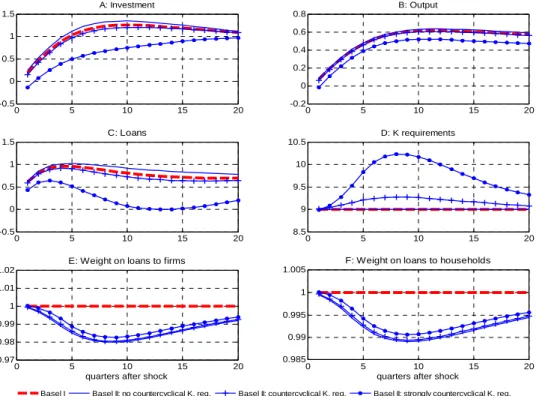
Figure 3 – Impulse responses with passive v countercyclical capital requirements 3.1 Positive technology shock
0 5 10 15 20 -0.5 0 0.5 1 1.5 A: Investment
Basel I Basel II: no countercyclical K. req. Basel II: countercyclical K. req. Basel II: strongly countercyclical K. req.
0 5 10 15 20 -0.2 0 0.2 0.4 0.6 0.8 B: Output 0 5 10 15 20 -0.5 0 0.5 1 1.5 C: Loans 0 5 10 15 20 8.5 9 9.5 10 10.5 D: K requirements 0 5 10 15 20 0.97 0.98 0.99 1 1.01 1.02
E: Weight on loans to firms
quarters after shock
0 5 10 15 20 0.985 0.99 0.995 1 1.005
F: Weight on loans to households
quarters after shock
3.2 Expansionary monetary policy shock
0 5 10 15 20 -0.1 0 0.1 0.2 0.3 0.4 A: Investment
Basel I Basel II: no countercyclical K. req. Basel II: countercyclical K. req. Basel II: strongly countercyclical K. req.
0 5 10 15 20 -0.05 0 0.05 0.1 0.15 B: Output 0 5 10 15 20 -0.1 0 0.1 0.2 0.3 0.4 C: Loans 0 5 10 15 20 8.9 9 9.1 9.2 9.3 9.4 D: K requirements 0 5 10 15 20 0.97 0.98 0.99 1 1.01 1.02
E: Weight on loans to firms
quarters after shock
0 5 10 15 20 0.985 0.99 0.995 1 1.005
F: Weight on loans to households
quarters after shock
Note: The impulse responses are measured as percentage deviations from steady state, except for the capital requirement (measured in percentage points); the responses of weights wi are normalised to 1 and measured in
levels. To ease the interpretation, in panel 2 the curves have been computed using a value of i in (5) five times
23
As usual, we start with a positive technology shock. Consider the responses of investment, in panel 3.1.A. The two top lines illustrate the reaction under Basel I (blue) and Basel II (dotted red). They are exactly those reported in Figure 1, for ease of comparison. The two new lines are obtained with a countercyclical management of the capital requirement – i.e. simulating the model augmented with equation (7). Specifically, the solid blue curve labelled ‘Basel II:
countercyclical K requirement’ is obtained by setting = 0.90 and = 20 in (7). The figure
clearly shows that this policy can undo the extra pro-cyclicality induced by Basel II relative to Basel I, and indeed, can improve upon Basel I. How is this stabilisation achieved? The basic mechanism is the same as illustrated in section 3. The stabilisation policy attenuates lending growth (panel C). In turn, this is due to the fact that the expansion of output drives up the
capital requirement t. The above parameterisation for and in (7) causes t to
gradually increase from its steady state of 9 percent to a maximum of 9.3 percent after about 8 quarters (panel D).
The response of output, in panel B, confirms this message from a qualitative viewpoint, although the small size of the effects, documented in section 3, causes the curves to be very similar. Notice that in this case the risk weights in panels E and F are hardly affected, and consequently play a minor role.
To assess the sensitivity of the results we simulated the model setting =100. The resulting
responses are labelled ‘Basel II: strongly countercyclical K requirement’. A look at the usual sequence of panels in figure 5.1 reveals significant changes. The responses of investment and output are now well below the Basel I benchmark, indicating that the attenuation of pro-cyclicality is now relatively marked. This effect is obtained with a 1.2 percentage point increase in the capital ratio, from the steady-state value of 9 percent to a peak of 10.2 percent after about two years. The order of magnitude of this increase is plausible.
According to the interpretation that we adopt in this section, equation 7 is a policy reaction function. Hence its parameters could be chosen optimally, so as to minimise pro-cyclicality, say, or maximise welfare. We leave this task for future research. The point of the simple exercise just described is to show that a countercyclical capital requirement policy can achieve relatively powerful results.
Panel 2 of Figure 3 replicates the exercise for a monetary policy shock. Overall, the results of panel 1 are qualitatively confirmed. As in previous sections, the difference across the different regulatory regimes turns out to be small for this type of shock. In this case, the ‘countercyclical K requirement’ policy manages to improve on the passive policy, but still leaves more pro-cyclicality than under the Basel I framework. To improve on the latter, the
‘strongly countercyclical K requirement’ policy should be adopted.22
Overall, our results suggest that introducing policy tools that allow building up and using buffers of resources in a countercyclical fashion may yield benefits, relative to an
22 As with previous cases, we also consider a demand shock. The results (not reported) confirm the analysis of
the previous sections. Conditioning on this type of shock, the success of the countercyclical K requirement policy is clear cut if one sticks to the strict definition of pro-cyclicality (output increases, and the increase is attenuated under the countercyclical policy); it is ambiguous if one considers the entire economy (loans and investment decline, and the decline is sharper under the countercyclical policy).
24
environment in which the only policy instrument is the interest rate. The practical implementation of this countercyclical capital requirements policy is the subject of section 6. As we shall see, such a policy need not be discretionary – i.e. its implementation need not require periodic meetings of a board, as it could be based on rules.
4.1.2 Would banks voluntarily adopt a countercyclical capital policy rule?
In our simplified framework, t can be thought of as comprising a buffer voluntarily held by
banks (e.g. to face unexpected losses) because the current version of the model does not distinguish between capital and provisions. Therefore, one may view equation 7 as an admittedly rough way to let banks – not the regulator – choose a (possibly countercyclical) capital buffer. Indeed, as mentioned above, various authors (Repullo and Suarez 2008 and Tarullo 2008) argue that forward-looking banks will find it optimal to manage their excess capital buffers in a countercyclical fashion, and that this endogenous response could
significantly offset the extra pro-cyclicality induced by the new regulations.23 If this were the
case, regulatory intervention on capital requirements could prove to be largely superfluous. A straightforward way to check whether this is the case within our framework is to look at bank profits (the interest rate margin, more precisely) under Basel II, with and without the countercyclical capital policy (7). Clearly, if banks can increase profits by voluntarily adopting countercyclical capital buffers, they will not wait for the regulator to intervene before implementing such a policy.
Figure 4 reports the impulse response of banks’ gross profits (i.e. before capital depreciation) to the usual technology and monetary policy shocks under the four regimes discussed in the previous section: the Basel I and Basel II regimes underlying Figures 1 and 2; and the Basel II regime with the countercyclical and ‘strongly’ countercyclical policy (7) underlying Figure 3. Look at the first panel, reporting the response of bank profits to a technology shock. Gauged with the yardstick of bank profits, the worst regime is Basel II with fixed capital buffers; next comes the Basel I regime; then, the Basel II with time-varying, countercyclical capital buffers (‘countercyclical K requirement’). The best is Basel II with strongly countercyclical K requirement. Thus, it seems that a countercyclical accumulation of voluntary capital buffers would be in the banks’ own interest.
Next, consider panel 2, reporting the response of profits to the expansionary monetary policy shock. Here the results become ambiguous. Specifically, the ordering of the curves depends on the time horizon: a policy of countercyclical capital build-up would initially harm profits. When a countercyclical policy is implemented, capital requirements are increased exactly when the capital/assets ratio falls because of the expansion in lending. As a consequence, the fall in bank loan rates induced by the expansionary monetary policy is partly offset by the increase in costs related to the banks’ capital position (see equation 2) and, consequently, profits fall by a larger amount. Overall, the figure suggests that banks would shy away from such a policy. As usual, we also considered a positive demand shock. The indications from the related figure (not reported) are in line with that of panel 1.
23 Repullo and Suarez (2008) suggest that these buffers would range from about 2 percent of total assets in
25
Summing up, several authors argue that, faced with the Basel II regulatory change, banks will find it optimal to offset the additional pro-cyclicality at least partially by appropriate voluntary capital buffers. Our analysis provides only partial support for this argument. As is often the case in the context of analyses conducted with DSGE models, the effectiveness of certain economic actions is not uniquely determined but conditional on the type of shock posited. As such, our results lend support to the view that a policy of countercyclical capital requirements, enforced by a regulator, would not be superfluous.
Figure 4 - Impulse responses of bank profits under alternative regulatory regimes
0 2 4 6 8 10 12 14 16 18 20
-10 -5 0 5
(1) Positive technology shock
0 2 4 6 8 10 12 14 16 18 20 -1.5 -1 -0.5 0 0.5 1 1.5
(2) Expansionary monetary policy shock
quarters after shock
Basel I Basel II: no countercyclical K. req. Basel II: countercyclical K. req. Basel II: strongly countercyclical K. req.
Note: The impulse responses are measured as percentage deviations from steady state. To facilitate interpretation, in panel 2 the curves have been computed using a value of i in (5) five times larger than the
baseline.
4.2 Increasing banks’ regulatory capital
Due to the crisis, proposals to raise the regulatory minimum capital above 8 percent and to improve capital quality have regained popularity. It is widely acknowledged that excessively low capital levels were helped to propagate the financial crisis. Relatively small losses, concentrated in time and affecting many intermediaries at once, triggered a deleveraging that had far-reaching consequences. Clearly, the adjustment could have been much less dramatic if the capital base had been larger – i.e. if the system’s leverage had been lower. However, in the current policy debate proposals to increase banks’ regulatory capital are seldom explicitly motivated with the need to reduce pro-cyclicality (see FSF 2008 and 2009 for example). This is probably due to the fact that the link between pro-cyclicality and the level of capital is not obvious. Intuitively, one could think that, as long as the cost borne for deviating from the
26
minimum requirement is unchanged, it is immaterial whether the minimum is set at 8 percent
or some much higher level.24
Within our model an increase in does have an effect on the dynamics of the key
macroeconomic variables.25 In more intuitive terms, the effect of ν on the system dynamics
may be seen as working through bank leverage: raising ν increases the steady-state value of
the capital/assets ratio, reducing leverage. While this should univocally attenuate the accelerator effect and therefore reduce pro-cyclicality, in practice we will see that the result is ambiguous. Thus, we have first assessed whether higher capital requirements increase or decrease pro-cyclicality. Next, we look at the macroeconomic costs of higher capital requirements.
For the first task, we use the baseline parameterisation of our model to compute impulse-response functions of bank variables and key macroeconomic variables to different shocks,
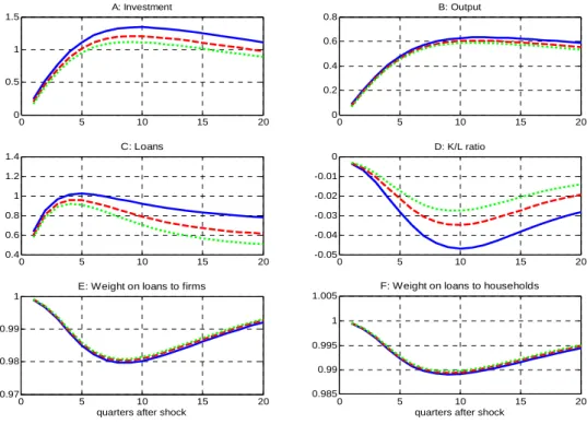
adopting several different, plausible values for . Figure 5.1, the counterpart of Figure 1,
reports the reaction to a positive technology shock. The curves labelled =0.09 are those of
the baseline exercises in Figure 1, reported for ease of comparison. The figure suggests that higher capital requirements attenuate the reaction of the key bank variables: the curves for
loans and the capital/assets ratio corresponding to higher are relatively closer to zero
(panels C, D).26 In turn, the dynamics of loans affect investment (panels B, C) and output.
Figure 5.2 replicates the same exercise for an expansionary monetary policy shock. Since under the baseline parameterisation the curves virtually overlap in all the panels, we plot the
responses obtained setting χi 5 times larger than the baseline; this magnifies the differences
without altering their sign. The results appear now to be reversed, although they are not clear-cut.
24 This point is well summarised by Brunnermeier et al. (2009): “requirements based on minimum capital
ratios do not provide resilience, since they cannot be breached. They represent a tax, not a source of strength”. Accordingly they suggest introducing higher target levels of capital, with a specific, rule-based ladder of increasing sanctions.
25 There are two indirect (and technical) effects. First, the depreciation parameter δ
b in equation (3) is
determined by the parameter ν (via a series of conditions discussed in Gerali et al. 2009, which we have omitted from section 2). Thus, increasing ν causes a decline in δb which affects the dynamics of capital
accumulation via (3). Second, looking at the log-linear approximation to equation 2 used to derive the impulse response functions presented throughout the paper, one can see that a higher implies that a given deviation of the capital/assets ratio has a greater effect on the interest rates set by banks.
26 The curves in Figure 3 are derived from models with different steady states. They are comparable because
27
Figure 5 - Impulse responses under different levels of capital requirements (1) positive technology shock
0 5 10 15 20 0 0.5 1 1.5 A: Investment
Basel II: = 0.09 Basel II: = 0.12 Basel II: = 0.15
0 5 10 15 20 0 0.2 0.4 0.6 0.8 B: Output 0 5 10 15 20 0.4 0.6 0.8 1 1.2 1.4 C: Loans 0 5 10 15 20 -0.05 -0.04 -0.03 -0.02 -0.01 0 D: K/L ratio 0 5 10 15 20 0.97 0.98 0.99 1
E: Weight on loans to firms
quarters after shock
0 5 10 15 20 0.985 0.99 0.995 1 1.005
F: Weight on loans to households
quarters after shock
(2) Expansionary monetary policy shock
0 5 10 15 20 -0.2 -0.1 0 0.1 0.2 0.3 A: Investment
Basel II: = 0.09 Basel II: = 0.12 Basel II: = 0.15
0 5 10 15 20 -0.05 0 0.05 0.1 0.15 B: Output 0 5 10 15 20 -0.1 0 0.1 0.2 0.3 0.4 C: Loans 0 5 10 15 20 -10 -5 0 5x 10 -3 D: K/L ratio 0 5 10 15 20 0.97 0.98 0.99 1 1.01 1.02
E: Weight on loans to firms
quarters after shock
0 5 10 15 20 0.985 0.99 0.995 1 1.005
F: Weight on loans to households
quarters after shock
Note: The impulse responses are measured as percentage deviations from steady state, except for the capital requirement (measured in percentage points); the responses of weights wi are normalised to one and measured in
levels. To facilitate interpretation, in panel (2) the curves have been computed using a value of i in (5) five