A Computation-Efficient CNN System for High-Quality Brain Tumor Segmentation

A Computation

-

Efficient CNN System for High

-

Quality Brain

Tumor Segmentation

Electrical and Computer Engineering

Presented in Partial Fulfillment of the Requirements for the Degree of Master of Applied Science at

Concordia University Montreal, Quebec, Canada

August 2020

CONCORDIA UNIVERSITY SCHOOL OF GRADUATE STUDIES

This is to certify that the thesis prepared By: Yanming Sun

Entitled: A Computation-Efficient CNN System for High-Quality Brain Tumor Segmentation

and submitted in partial fulfillment of the requirements for the degree of

Master of Applied Science (Electrical and Computer Engineering)

complies with the regulations of this University and meets the accepted standards with respect to originality and quality.

Signed by the final examining committee:

________________________________________________ Chair Dr. W.-P. Zhu

________________________________________________ External Examiner Dr. A. Ben Hamza (CIISE)

________________________________________________ Internal Examiner Dr. W.-P. Zhu

________________________________________________ Supervisor Dr. C. Wang

Approved by: ___________________________________ Dr. Y.R. Shayan, Chair

Department of Electrical and Computer Engineering

_______________ 20___ __________________________________ Dr. Mourad Debbabi, Interim Dean,

Gina Cody School of Engineering and Computer Science

iii

Abstract

A Computation-Efficient CNN System for High-Quality Brain Tumor Segmentation Yanming Sun

Brain tumor diagnosis is an important issue in health care. Automated brain tumor segmentation can help timely diagnosis. It is, however, very challenging to achieve high-quality segmentation results, because the shapes, sizes, textures and locations of brain tumors vary from patient to patient. To develop a Convolutional Neural Network (CNN) system for a high-quality brain tumor segmentation at the lowest computation cost, the CNN should be custom-designed to extract efficiently sufficient critical features particularly related to the tumors from brain images for the multi-class segmentation of tumor areas.

In this thesis, a CNN system is proposed for brain tumor segmentation. The system consists of three parts, a pre-processing block to reduce the data volume, an application-specific CNN (ASCNN) to segment tumor areas precisely, and a refinement block to detect false positive voxels. The CNN, designed specifically for the task, has 7 convolution layers, and the number of output channels per layer is no more than 16. The convolutions combined with max-pooling in the first half of the CNN are performed to localize brain tumor areas. Two convolution modes, namely depthwise convolution and standard convolution, are performed in parallel in the first 2 layers to extract elementary features efficiently. In the second half of the CNN, the convolutions combined with upsampling are to segment different tumor areas. For a fine classification of pixel-wise precision, the feature maps are modulated by adding the weighted local feature maps generated in the first half of the CNN. The system has only 11716 parameters to be trained and, for a patient case of (240x240x155 x3) voxels, it requires only 21.14G Flops to complete the test. Hence, it is likely the simplest CNN system, so far reported, for brain tumor segmentation.

The performance of the proposed system has been evaluated by means of CBICA Image Processing Portal with samples from dataset BRATS2018. Requiring a very low computation volume, the proposed system delivers a high segmentation quality indicated by its average Dice scores of 0.75, 0.88 and 0.76 for enhancing tumor, whole tumor and tumor core, respectively, and the median Dice scores of 0.85, 0.92, and 0.86. Its processing quality is comparable to the

iv best ones so far reported. The consistency in system performance has also been measured, and the results have demonstrated that the system is able to reproduce almost the same output to the same input after retraining.

In conclusion, the proposed CNN system has been designed to meet the specific needs to segment brain tumors or other kinds of tumors in medical images. In this way, the redundancy in computation can be minimized, the information density in data flow increased, and the computation efficiency/quality improved. This design demonstrates that a CNN system can be made to perform a high-quality processing, at a very low computation cost, for a specific application. Hence, ASCNN is an effective approach to lower the barrier of computation resource requirement of CNN systems in order to make them more implementable and applicable for general public.

v

Acknowledgements

I would like to express my best appreciation to my supervisor Dr. Chunyan Wang for her support during my study in Concordia University. She always gives me brilliant guidance. Moreover, her focus on details in research influences me deeply. It is my great honor and fortune to work under her supervision.

I would also like to thank my colleagues, Yunlong Ma, Bao Zhu, and Mingze Ni, for the help in the last two years.

vi

Contents

List of Figures ... viii

List of Tables ... xi

List of Acronyms and Abbreviations ... xii

List of Symbols ... xiii

1. Introduction ... 1

1.1 Background and Challenges ... 1

1.2 Motivation and Objective ... 3

1.3 Scope and Organization ... 4

2. Background and Relevant Work ... 6

2.1 Introduction ... 6

2.2 Fundamentals of CNN ... 6

2.2.1 2D Convolution and Convolution Modes ... 6

2.2.2 Critical Components for CNN ... 8

2.2.3 Basic Blocks for CNN ... 11

2.2.4 Training Process and Important Setups ... 13

2.3 CNNs for Brain Tumor Segmentation ... 14

2.3.1 U-Net Based CNNs for Brain Tumor Segmentation ... 14

2.3.2 Other Forms of CNN for Brain Tumor Segmentation ... 19

2.4 Summary ... 20

3. Proposed System... 22

3.1 Introduction ... 22

3.2 Pre-Processing – Reduction of Data Volume ... 23

vii

3.2.2 Detection and Removal of Tumor-Free Slices ... 26

3.3 CNN ... 28

3.4 Post-Processing – Refinement ... 33

3.5 Summary ... 34

4. Performance Evaluation ... 35

4.1 Introduction ... 35

4.2 Dataset and Training ... 35

4.2.1 Dataset ... 35

4.2.2 Training Details ... 36

4.3 Testing and Performance Evaluation ... 37

4.3.1 Performance Metrics ... 37

4.3.2 Testing Results ... 39

4.3.3 Compare with State-of-the-Art Methods ... 50

4.4 Summary ... 52

5. Conclusion ... 54

viii

List of Figures

FIGURE 1.1COMPLICATED STRUCTURE OF HUMAN BRAIN [1]. ... 1

FIGURE 1.2T2 SLICES FROM TWO PATIENT CASES.(A)HGG/BRATS18_2013_2_1,NO.91ST SLICE. (B)HGG/BRATS18_2013_7_1,NO.101ST SLICE. ... 2

FIGURE 1.3 BRAIN IMAGES AND GROUND TRUTH OF TUMOR FROM TWO PATIENT CASES. THE IMAGES IN THE FIRST ROW ARE FLAIR, T1, T1C, T2 AND GROUND TRUTH OF PATIENT BRATS18_2013_2_1; THE IMAGES IN THE SECOND ROW ARE THOSE OF PATIENT BRATS18_2013_7_1. ... 3

FIGURE 2.1AN EXAMPLE OF 2D CONVOLUTIONS. ... 7

FIGURE 2.2CURVE OF RELU. ... 9

FIGURE 2.3AN EXAMPLE CURVE OF LEAKY RELU, 𝛼 = 0.2. ... 9

FIGURE 2.4CURVE OF SIGMOID FUNCTION. ... 10

FIGURE 2.5INPUT AND OUTPUT OF POOLING, STRIDE 2. ... 10

FIGURE 2.6ARCHITECTURE OF VGG[11]. ... 11

FIGURE 2.7ARCHITECTURE OF SEGNET [12]. ... 12

FIGURE 2.8ARCHITECTURE OF INCEPTION BLOCK [13]. ... 12

FIGURE 2.9ARCHITECTURE OF DEEP RESIDUAL BLOCK [15]. ... 13

FIGURE 2.10ARCHITECTURE OF THE DENSELY CONNECTED BLOCK [16]. ... 13

FIGURE 2.11ARCHITECTURE OF U-NET [22]. ... 15

FIGURE 2.12 DETAILS OF THE CNN IN [23]. (A) BASIC ARCHITECTURE. (B) DETAILS OF THE WEIGHTED ADDITION.(C)DETAILS OF THE INCEPTION BLOCK. ... 16

FIGURE 2.13STACKED U-NET [24]. ... 16

FIGURE 2.14DETAILS OF DRINET [25].(A)BASIC ARCHITECTURE.(B)DENSE CONNECTION BLOCK. (C)RESIDUAL INCEPTION BLOCK. ... 17

FIGURE 2.15DETAILS OF THE CNN IN [26].(A)BASIC ARCHITECTURE.(B)RECOMBINATION BLOCK. (C)RECOMBINATION AND RECALIBRATION BLOCK. ... 18

FIGURE 2.16.ARCHITECTURE OF THE NETWORK PRESENTED IN [27]. ... 19

FIGURE 2.17FLOWCHART OF THE CNN PRESENTED IN [28]... 19

ix FIGURE 2.19.FLOWCHART OF THE CNN REPORTED IN [31]. ... 20

FIGURE 3.1OVERVIEW OF THE PROPOSED SYSTEM.THERE ARE FOUR 3D IMAGES NAMELY FLAIR,

T1, T1C AND T2 IN EACH PATIENT CASE, AND THE SIZE OF THE 3D BRAIN IMAGES IS

240×240×155. ... 22 FIGURE 3.2(A)FLAIR SLICE.(B)T1 SLICE.(C)T1C SLICE.(D)T2 SLICE.(E)GROUND TRUE. ... 23

FIGURE 3.3(A)EXAMPLE OF THE ORIGINAL INPUT SLICES SIZED 240×240 PIXELS.(B)SLICE AFTER THE MARGIN REMOVAL, SIZED 168×200 PIXELS. ... 25

FIGURE 3.4HISTOGRAMS OF X1, X2, Y1 AND Y2OF BRATS2018 TRAINING SET ... 25 FIGURE 3.5EXAMPLES OF SLICES WITH HIGH PERCENTAGE OF BACKGROUND PIXELS. ... 26

FIGURE 3.6(A)AN EXAMPLE OF A FLAIR SLICE WITHOUT TUMOR.(B)AN EXAMPLE OF A FLAIR SLICE WITH TUMOR.(C)UPPER AND LOWER HALVES OF THE CONTENTS IN (A).(D)UPPER AND LOWER HALVES OF THE CONTENTS IN (B). ... 27

FIGURE 3.7(A)(B)EXAMPLES OF SLICES WITH INCOMPLETE BRAIN AREAS.(C)UPPER AND LOWER HALVES OF THE BINARY IMAGE OF (A) THAT HIGHLIGHTS THE OUTLINE OF THE BRAIN AREA.(D)

UPPER AND LOWER HALVES OF THE BINARY IMAGE OF (B). ... 27

FIGURE 3.8EXAMPLE OF THE INPUT AND OUTPUT OF THE PROPOSED CNN.(A)~(D)FLAIR,T1,T1C AND T2 SLICE SAMPLES. IN EACH SLICE, THE INTENSITY VALUES ARE CHANNEL-WISELY NORMALIZED.(E)GROUND TRUTH.(F)EXAMPLE OF PREDICTED RESULT. ... 29

FIGURE 3.9.DETAILED DIAGRAM OF THE PROPOSED CNN. ... 30

FIGURE 4.1LOSS CURVE IN THE TRAINING PROCESS OF THE PROPOSED SYSTEM... 37

FIGURE 4.2SLICE OF SEGMENTED BRAIN IMAGE TO INDICATE THE LESION. T1 IS THE NUMBER OF

PIXELS IN THE TRUE LESION REGION, WHICH IS LOCATED IN THE RED-CONTOURED AREA.P1 IS

THE NUMBER OF PIXELS IN PREDICTED LESION REGION, WHICH IS LOCATED IN THE BLUE -CONTOURED AREA. T0 AND P0 ARE THE NUMBER OF PIXELS IN NORMAL REGIONS IN THE

GROUND TRUTH AND THE PREDICTED MAPS, RESPECTIVELY. ... 38

FIGURE 4.3DISTRIBUTIONS OF DICE SCORES IN ET AREAS OBTAINED IN THE TEN EXPERIMENTS... 41

FIGURE 4.4DISTRIBUTIONS OF DICE SCORES IN WT AREAS OBTAINED IN THE TEN EXPERIMENTS. 41

FIGURE 4.5DISTRIBUTIONS OF DICE SCORES IN TC AREAS OBTAINED IN THE TEN EXPERIMENTS. . 42

FIGURE 4.6BOXPLOTS OF THE TEST RESULTS OBTAINED IN THE TEN EXPERIMENTS. ... 42

FIGURE 4.7FOUR INPUT SLICES (THE 96TH) OF CASE 1 AND THE PREDICTED TUMOR LOCATIONS. . 48

x FIGURE 4.9FOUR INPUT SLICES (THE 53RD) OF CASE 3 AND THE PREDICTED TUMOR LOCATIONS. . 49

FIGURE 4.10FOUR INPUT SLICES (THE 57TH) OF CASE 4 AND THE PREDICTED TUMOR LOCATIONS. 49

FIGURE 4.11FOUR INPUT SLICES (THE 110TH) OF CASE 5 AND THE PREDICTED TUMOR LOCATIONS.

... 50 FIGURE 4.12FOUR INPUT SLICES (THE 86TH) OF CASE 6 AND THE PREDICTED TUMOR LOCATIONS. 50

xi

List of Tables

TABLE 3.1DETAILS OF THE CNN CONFIGURATION ... 31

TABLE 4.1PARTITION OF THE SAMPLES FROM DATASET BRATS2018... 35

TABLE 4.2STATISTICAL DATA OF THE TEN EXPERIMENTS ... 43

TABLE 4.3MEAN SCORES OBTAINED IN THE TEN EXPERIMENTS ... 43

TABLE 4.4TEST RESULTS OF 44BIG ENHANCING TUMOR (BET) CASES IN EXPERIMENT 5 ... 45

TABLE 4.5TEST RESULTS OF 22SMALL ENHANCING TUMOR (SET) CASES IN EXPERIMENT 5 ... 46

TABLE 4.6INFORMATION OF SIX PATIENT CASES ... 47

TABLE 4.7TEST RESULTS OF CASE 1 OBTAINED IN THE TEN EXPERIMENTS ... 48

TABLE 4.8TEST RESULTS OF CASE 2 OBTAINED IN THE TEN EXPERIMENTS ... 48

TABLE 4.9TEST RESULTS OF CASE 3 OBTAINED IN THE TEN EXPERIMENTS ... 49

TABLE 4.10TEST RESULTS OF CASE 4 OBTAINED IN THE TEN EXPERIMENTS ... 49

TABLE 4.11TEST RESULTS OF CASE 5 OBTAINED IN THE TEN EXPERIMENTS ... 50

TABLE 4.12TEST RESULTS OF CASE 6 OBTAINED IN THE TEN EXPERIMENTS ... 50

TABLE 4.13COMPARISON OF THE RESULTS –DICE,SENSITIVITY,SPECIFICITY AND HAUSDORFF95 ... 51

xii

List of Acronyms and Abbreviations

Adam Adaptive moment estimation

ASCNN Application-Specific Convolutional Neural Network

BN Batch Normalization

BRATS The Multimodal Brain Tumor Image Segmentation Benchmark CBICA Center for Biomedical Image Computing and Analytics

CNN Convolutional Neural Network

ET Enhancing tumor

FCN Fully Convolutional Network

FDR False Discovery Rate

FLAIR Fluid-attenuated inversion recovery

FLOPs Floating-Point Operations

FNR False Negative Rate

HGG High-grade gliomas

LGG Low-grade gliomas

MRI Magnetic Resonance Imaging

ReLU Rectified Linear Unit

SGD Stochastic gradient descent

T1 T1-weighted imaging

T1c T1-weighted contrast-enhanced imaging

T2 T2-weighted imaging

TC Tumor core

VGG Visual Geometry Group

xiii

List of Symbols

Nsl The number of slices per 3D images.

NvET The number of voxels in ET areas

P0 Number of voxels in the tumor-free regions in a predicted image

P1 Number of voxels in the tumor regions in a predicted image

StdDev Standard deviation

T0 Number of voxels in the tumor-free regions in the ground truth

T1 Number of voxels in the tumor regions in the ground truth

w(k1, k2) 2D kernel

x00, x01, …, x33 Input of pooling operation

x1 The distance between the left boundary of a slice and the leftmost point of

the brain area.

x2 The distance between the right boundary of a slice and the rightmost

point of the brain area.

x(i, j) Input image of 2D convolution

y00, y01, y10, y11 Output of pooling operation

y1 The distance between the upper boundary of a slice and the uppermost

point of the brain area.

y2 The distance between the lower boundary of a slice and the lowermost

point of the brain area.

𝑦_𝑖 The predicted probability

y(i, j) Output image of 2D convolution

𝑦_𝑡 The label of the ground truth x1m, x2m, y1m and y2m A fixed set of x1, x2, y1 and y2.

1

1.

Introduction

1.1 Background and Challenges

Brain tumors pose a serious problem to human health, and brain tumor segmentation is a critical step for the diagnosis and treatment of the disease. Manual segmentation is very time-consuming and often causes delays. It is thus important to develop fully automated computer vision systems for brain tumor segmentation to facilitate timely diagnosis. This development is, however, a very challenging task.

Human brain is likely the most complex organ in human body. From anatomy point of view, it is composed of many interconnected areas, each of which has different structures and specialized for different functions, as illustrated in Figure 1.1. Brain tumors can have many different types, growing in different parts of a brain. Each type of tumors can have different appearances in different stages of its development.

Figure 1.1 Complicated structure of human brain [1].

From computer vision point of view, human brain is a complicated 3D structure and is often represented as a large number of slices from different cross-sections. Voxels in the 3D structure

2 are represented by the pixels in the 2D slices. The structures of tissues in slices are interpreted as different textures, as examples illustrated in Figure 1.2.

(a) (b)

Figure 1.2 T2 slices from two patient cases. (a) HGG/Brats18_2013_2_1, No. 91st _{slice. (b) HGG/Brats18_2013_7_1, No. 101}st _slice.

A computer vision program for brain tumor segmentation needs to be able to distinguish tumor tissue from healthy tissue. In practice, tumor tissues in one location can have similar texture to that of healthy tissues in another location, whereas two tumor areas in different locations may have very different patterns, as illustrated in Figure 1.3. One cannot identify tumor areas by applying a simple pattern detection method. Moreover, for meaningful applications in brain tumor diagnosis, the computer vision program needs to define whole-tumor regions and to classify the voxels in these regions into multiple classes, corresponding to three types of intra-tumoral structures, namely edema, non-enhancing (solid) core/necrotic (or fluid-filled) core and enhancing core [2]. This multi-class classification in voxel-wise precision makes the development of a fully automated systems for brain tumor segmentation even more challenging.

3 Figure 1.3 Brain images and ground truth of tumor from two patient cases. The images in the first row are FLAIR, T1, T1c, T2 and ground truth of patient Brats18_2013_2_1; The images in the second row are those of patient Brats18_2013_7_1.

1.2 Motivation and Objective

Like most of object detection or recognition programs, a computer vision program for brain tumor segmentation involves 2 basic functions of image processing, feature extraction and classification. The feature extraction is often based on 2D filtering, and the critical issue is how to catch effectively all the image features useful for this specific classification, while these features are often mixed up with everything else. The quality of the feature extraction can have a critical effect on the quality of the classification, though the latter is also related to other elements in the system design.

Brain tumor segmentation can be done by means of filtering and/or morphological operations. High-pass and/or band-pass filters can be applied to extra features. The segmentation method reported in [3] is based on feature extracted by applying Sobel high-pass filtering method. Tumor features can also be extracted by applying Gabor filters, and the data are used to classify the pixels with extremely randomized trees [4]. As healthy brains have certain degree of symmetry [5], brain tumor detection can be done by analysing the symmetry of MRI brain images [6]. Implementations of these methods do not require a large number of computation resources. However, due to the complexity of the brain tumor variations, it is difficult to precisely classify the pixels of intra-tumoral structures.

4 Convolutional Neural Networks (CNNs) are widely used for feature extraction and classification in various data processing applications, including those for medical image segmentations. A large number of research papers are found in literature about CNN systems for brain tumor segmentation. The processing quality reported in most of the papers is superior, with respect to that achieved by conventional filtering methods, however, CNN systems require much more computation resources. Most of them have millions, if not tens of millions, of parameters. Considering the large amount of data in a 3D input image, a huge volume of computation is required for such a system to perform a test of a single case, and its training process is even much more computation consuming. Hence, to train and to use the systems, one needs a powerful computing facility, which can limit the implementation and applications of the CNN systems for brain tumor segmentation.

The objective of the work presented in this thesis is to design a fully automated computer vision system for high-quality brain tumor segmentation with low computation requirement in order to facilitate its implementation. The system involves a CNN block for feature extraction and classification. The design of the CNN aims at a simplicity in structure and efficiency in its operations. To this end, the CNN system should be an Application Specific CNN (AS-CNN), i.e., custom-designed for specific applications, instead of general-purpose.

1.3 Scope and Organization

To extract various features from the input images and precisely classify the pixels/voxels for a specific application, without requiring a large amount of computation, the CNN should be custom-designed to target the specific features in the input data and to generate the output data useful in the application. The CNN system to be proposed in this thesis will consist of 3 blocks.

• Pre-processing block for data reduction so that the data processed in the succeeding CNN block will have a much smaller amount and a higher density of feature information with respect to the original input data.

• CNN for feature extraction and classification.

5 The pre and post processing blocks will be designed aiming at reducing the computation burden of the CNN so that it can be made to perform the feature extraction and classification more effectively and efficiently.

The thesis is organized as follow. Description of CNN basics and a brief review of the existing systems for brain tumor segmentation are found in Chapter 2. The proposed CNN system is presented in Chapter 3 with detailed description of the design of each functional block. Chapter 4 is dedicated to a comprehensive performance evaluation of the proposed system. The training process and the test results are presented. The performance of the system is compared to those of the CNNs reported in recent years, which is also found in Chapter 4. Chapter 5 is a conclusion of the work presented in this thesis.

6

2.

Background and Relevant Work

2.1 Introduction

Since brain tumor segmentation is very challenging, many efforts are devoted to this task. A large number of methods for this task have been developed, include filtering systems/morphological operations and Convolutional neural networks. In general, Filtering systems/morphological operations are very computation-efficient, but it is difficult to detect a variety of features in brain images. On the contrary, CNNs require huge amount of computation volume but have high potential to handle the problem if there are adequate training samples. Thus, the work in this thesis is focused on computation-efficient CNN system.

In this chapter, the fundamentals of CNN are shown in sub-chapter 2.2. The CNNs for brain tumor segmentation reported recent years are given in sub-chapter 2.3. A brief summary is presented in sub-chapter 2.4.

2.2 Fundamentals of CNN

A CNN is mainly composed of convolution operations, combined with other critical elements, e.g., normalization, non-linear activation function and pooling. Different from traditional convolution operations, the kernels of the convolutions in a CNN are not deterministic. They shall be trained by using a large number of samples.

2.2.1 2D Convolution and Convolution Modes

A 2D convolution is in fact a filtering operation, it is defined as follow:

𝑦(𝑖, 𝑗) = ∑𝑛_{𝑘1=−𝑛}∑𝑚_{𝑘2=−𝑚}𝑤(𝑘₁, 𝑘₂)𝑥(𝑖 − 𝑘₁, 𝑗 − 𝑘₂) (2.1) where 𝑤 is a 2D kernel; x and y are input and output and their dimensions are (2n+1, 2m+1). There are three types of 2D filter, high-pass filter, low-pass filter and band-pass filter. An example of a high-pass filter (Sobel filter) is shown in Figure 2.1.

7 Input image Kernel 1 Output image 2 Kernel 2 Output image 1

Figure 2.1 An example of 2D convolutions.

Deterministic kernels can extract specific features in the input images, e.g., the two kernels in Figure 2.1 are to extract vertical edges and horizontal edges of the input image, respectively. It is not easy to design a large number of different deterministic kernels to extract variant features in brain images. However, a CNN has multi-layer convolutions, and there are multiple channels in each layer. More importantly, unlike the deterministic convolutions in Figure 2.1, the kernels in the CNN are trainable, and they can be determined by a training process. Thus, CNN is a more feasible choice for brain tumor segmentation.

As mention above, the convolution in CNN has multiple channels in each layer. There are three types of convolution modes for the channels in a layer. Assume the kernel size is 3×3, and the numbers of input and output channels are 16 and 32, respectively:

(1) Standard convolution. In this mode, each of the output channels is produced by all of the input channels, so the number of weights in this layer is 4608 (3×3×16×32).

8 (2) Group convolution. Assume the input channels are divided into 4 groups, then a group convolution is similar to 4 small-scale standard convolutions. The number of weights in this layer is 1152 (3 × 3 ×16

4 × 32

4 × 4).

(3) Depthwise convolution. In this mode, each of the output channels is produced by only one of the input channels. Since the number of the output channels is twice that of the input channels, an input channel should produce two output channels. The number of weights in this layer is 288 (3×3×32).

2.2.2 Critical Components for CNN

Except the convolutions, there are many other components in CNN architecture.

(1)Normalization. A normalization is to uniform the range and the distribution of the data in each layer, thereby facilitating the convergence of a network.

(i) Batch normalization (BN) [7]. A BN normalizes the feature maps by using the mean and standard deviation of a whole batch of data.

(ii)Channel-wise normalization. The data of each channel are normalized with the mean and the standard deviation of the channel.

(2)Non-linear activation function. The relationship between the input and the output in image segmentation is non-linear. However, the convolution is a linear function. Thus, it is necessary to introduce non-linearity to help a network learn complex data and to provide accurate predictions.

(i) Rectified Linear Unit (ReLU) [8]. ReLU is a non-linear activation function defined as 𝑓(𝑥) = 𝑚𝑎𝑥⁡(0, 𝑥). It is the most computation-efficient activation function so far. The curve of ReLU is shown in Figure 2.2. It should be noted that only positive values can be perform backpropagation.

9 Figure 2.2 Curve of ReLU.

(ii)Leaky ReLU [9]. Leaky ReLU is defined as 𝑓(𝑥) = 𝑚𝑎𝑥⁡(𝛼𝑥, 𝑥), where 𝛼 is a constant and 0 < 𝛼 < 1. It has a small positive slope 𝛼 in the negative area, so it enables backpropagation for both positive values and negative values, as shown in Figure 2.3.

Figure 2.3 An example curve of Leaky ReLU, 𝛼 = 0.2.

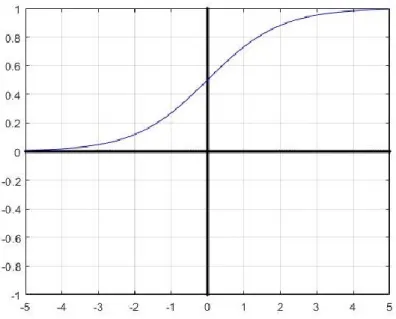
(iii) Sigmoid [10]. Sigmoid function is also called Logistic Activation Function. It is defined as 𝑓(𝑥) = 1

(1+𝑒−𝑥₎ . The curve of Sigmoid is shown in Figure 2.4. The range of the values of sigmoid function is from 0 to 1. It leads to a vanishing gradient problem when the input data has very high absolute value.

10 Figure 2.4 Curve of Sigmoid function.

(3)Pooling. A pooling operation is in fact a downsampling. It is to increase signal density, to reduce data volume and to decrease computation complexity. Max pooling and average pooling are widely used in practical.

(i) Max pooling. Assume the stride is equaled to 2, a maximum value of four adjacent pixels will be reserved, and the other three pixels will be removed, so the number of pixels of the output is a quarter of that of the input. As shown in Figure 2.5, the output is 𝑦₀₀= 𝑚𝑎𝑥⁡(𝑥₀₀, 𝑥₀₁, 𝑥₁₀, 𝑥₁₁) , …, 𝑦₁₁ = 𝑚𝑎𝑥⁡(𝑥22, 𝑥23, 𝑥32, 𝑥33).

(ii)Average pooing. An average pooling means that an average value of four adjacent pixels will be reserved. As showed in Figure 2.5, the output is 𝑦00 = (𝑥00+

𝑥₀₁+ 𝑥₁₀+ 𝑥₁₁)/4, …, 𝑦₁₁= (𝑥₂₂+ 𝑥₂₃+ 𝑥₃₂+ 𝑥₃₃)/4.

Input Output

11 (4) Upsampling. The size of the output image of a CNN for image segmentation is the same as that of the input image. After pooling the input data, upsampling operations should be used to recover the dimension of the data. There are two widely used upsampling methods, nearest-neighbor interpolation and bilinear interpolation.

2.2.3 Basic Blocks for CNN

In this sub-chapter, serval widely used blocks of CNN are given.

(1)VGG [11]. VGG is proposed by Visual Geometry Group at University of Oxford. There are two versions of VGG architecture. The first one is VGG16, i.e., there are 13 convolution layers and 3 fully connected layers, as shown in Figure 2.6. The other one is VGG19, which has 19 layers. All the convolution layers in VGG blocks are standard convolution with 3×3 kernel. In addition, ReLU and max pooling are applied to the blocks. The VGG block is widely used in image segmentation, for example, SegNet [12]. It has a so-call encoder-decoder architecture, which is shown in Figure 2.7. The encoder is in fact a VGG16 without fully connected layer. The decoder is a flipped VGG16 without fully connected layer.

12 Figure 2.7 Architecture of SegNet [12].

(2)Inception block [13][14]. There are three kernels with different sizes performed in parallel. Large kernel is to extract global features, and small kernel is to extract local features.

Figure 2.8 Architecture of inception block [13].

(3)Deep residual block [15]. Very deep neural networks are difficult to train and will cause low predicted accuracy. Deep residual block has shortcut connections to enable a network to be deeper. Its architecture is given in Figure 2.9.

13 Figure 2.9 Architecture of deep residual block [15].

(4)Densely connected block [16]. The architecture of densely connected block is shown in Figure 2.10, the feature-maps of all preceding layers are used as inputs of all subsequent layers, so that the connection between layers is very dense. Thus, the network can be deeper.

Figure 2.10 Architecture of the densely connected block [16].

2.2.4 Training Process and Important Setups

After building a CNN architecture, the trainable parameters should be determined by training process. The training process includes forward propagation and backward propagation. (i) Forward propagation means that the CNN produces a predicted result based on the input data. (ii) Backward propagation means that a loss is calculated based on the predicted results and the ground truth, and the trainable parameters in the CNN are updated according to the loss.

14 There are many critical setups for training processing.

(1)Batch size. A batch of input images should be plentiful enough to contain variance features. However, the upper limit of the batch size is related to the volume of a dataset. In other word, the dataset should be divided into adequate batches to let the network update step by step.

(2)Loss function. Cross-Entropy loss is widely used in CNN [17]. It is defined as

𝐿𝑜𝑠𝑠 = ⁡ ∑ −𝑦_𝑡𝑙𝑜𝑔⁡(𝑦_𝑖) (2.2) where 𝑦_𝑡 is the label of the ground truth, and 𝑦_𝑖 is the predicted probability.

(3)The number of training epochs. The training processing cannot be stopped before the loss curve converges.

(4)Learning rate. Learning rate should be large in the initial stages to adjust the network coarsely, and it should be small in the last stages to finely adjust the network.

(5)Data augmentation [18]. To train a CNN meaningfully, the training set should contain adequate features. However, the number of samples in training set is limited in most datasets. Thus, data augmentation can be performed to increase the number of samples for training. It includes flipping and rotating the input images.

(6)Optimizer. Stochastic Gradient Descent (SGD) [19] and Adaptive Moment Estimation (Adam) [20] are widely used in CNN. Adam is computation-efficient and is suitable for large network and huge data volume.

2.3 CNNs for Brain Tumor Segmentation

A lot of CNN systems for brain tumor segmentation have been reported. Many of them are designed based on the famous U-net.

2.3.1 U-Net Based CNNs for Brain Tumor Segmentation

U-net, designed based on FCN [21], has been widely used in medical image processing, including brain tumor segmentation [22]. The architecture of net is shown in Figure 2.11. U-net consists of a VGG-like contracting path, and an expansive path, in which copies of the feature data generated in the contracting path are included, by concatenation, in the convolutions.

15 Figure 2.11 Architecture of U-net [22].

A large number of U-net-based CNN systems for brain tumor segmentation have been reported in recent years, attempting to improve the segmentation quality.

In the CNN presented in [23], standard convolution blocks in the original U-net are replaced by inception blocks. Also, up skip connection is used to enhance network connectivity. The details of the CNN are shown in Figure 2.12.

16 Figure 2.12 Details of the CNN in [23]. (a) Basic architecture. (b) Details

of the weighted addition. (c) Details of the inception block.

U-net structure can be also used as a basic block, and multiple blocks are stacked to seek a better processing quality [24]. The architecture of this network is given in Figure 2.13. These basic blocks are simplified from U-net, and the so call ‘bridge connections’ are used to connect

these blocks.

17 In DRINet [25], which details are shown in Figure 2.14, standard convolution blocks in the first layers are replaced by dense connection blocks, and those in the last layers are replaced by residual inception blocks, whereas the copy/crop part (also called long skip connection) is not used.

(a)

(b)

Figure 2.14 Details of DRINet [25]. (a) Basic architecture. (b) Dense connection block. (c) Residual inception block.

The network presented in [26] was designed to have recombination of features and spatially adaptive recalibration block to improve the segmentation quality. The details of the CNN are presented in Figure 2.15.

18 (a)

(b)

(c)

Figure 2.15 Details of the CNN in [26]. (a) Basic architecture. (b) Recombination block. (c) Recombination and Recalibration block.

19

2.3.2 Other Forms of CNN for Brain Tumor Segmentation

Except the U-net-based CNNs, other forms of CNN can also be adopted for brain tumor segmentation.

In the network reported in [27], the structure of deep residual network is used and combines with spatial fusion blocks. Also, the middle supervision block is applied at the last stage. The architecture is shown in Figure 2.16.

Figure 2.16. Architecture of the network presented in [27].

The network in [28] is an architecture of multiple convolution pathways, which is presented in Figure 2.17. It is made to operate with patches obtained from axial, coronal and sagittal views of the 3D MRI brain images.

20 DeepMedic [29] and DF-MLDeepMedic network [30] are CNNs with two 3D convolution pathways, to extract local and larger contextual features, respectively. The flowchart is shown in Figure 2.18. The 3D system presented in [31] involves dense connectivity structure, feature pyramid module, and deep supervision mechanism to improve the segmentation quality. It should be noted that, the convolutions in these 3D systems are performed with 3D input data, and thus 4D kernels are used in a convolution involving multiple channels, which requires more parameters to be trained with respect to standard 2D convolution.

Figure 2.18 Flowchart of the CNN reported in [29][30].

Figure 2.19. Flowchart of the CNN reported in [31].

2.4 Summary

In this chapter, a brief description of the fundamentals of CNN is given. It includes (i) the principle of 2D convolution and three convolution modes; (ii) the critical components of CNN, e.g., normalization, non-linear activation function, pooling and upsampling; (iii) basic blocks for CNN, like VGG, inception block, deep residual block and densely connected block, and (iv) training process and important setups for training.

21 In addition, the CNNs for brain tumor segmentation reported in recent years are presented in this chapter. Many of them are U-net-based network. Most of them increase the computation complexity in order to improve the segmentation quality.

Based on these investigation results, the work in this thesis will adopt the basic architecture of U-net, but the details are custom-design based on the characters of input signals to yield high-quality segmentation under low computation complexity.

22

3.

Proposed System

3.1 Introduction

Automated brain tumor segmentation is an important processing for timely diagnosis in order to optimize treatments. In the design of the proposed system, the emphasis is to achieve a good segmentation quality at the lowest computation cost in order to facilitate its implementation. The basic block diagram of the system is shown in Figure 3.1.

The input of the proposed system is 3D brain images. The case of each patient is represented by four 3D images, namely FLAIR, T1, T1c and T2, as shown in Figure 3.1. Each of the 3D images is sliced into 2D slices. Hence, a voxel in a 3D image becomes a pixel in a 2D slice, and the brain tumor segmentation of 3D images is done by segmenting these 2D slices. An example of the 2D slices is shown in Figure 3.2 (a)~(d), and the ground truth of the brain tumor segmentation corresponding to these slices is shown in Figure 3.2 (e). It is difficult to find a deterministic model that can be used to detect various brain tumors in a pixel-wise precision. CNN can be potentially useful to handle such a problem if there is an appropriate dataset for training and testing the system.

CNN Pre-processing Data Reduction 155 slices FLAIR T1 T1c T2 Output 155 slices Slice size 240×240 Slice size 240×240 Slice size: 168×200; Number of Slices: <155 Post-processing Refinement

Figure 3.1 Overview of the proposed system. There are four 3D images namely FLAIR, T1, T1c and T2 in each patient case, and the size of the 3D brain images is 240×240×155.

23

(a) (b)

(c) (d)

(e)

Figure 3.2 (a) FLAIR slice. (b) T1 slice. (c) T1c slice. (d) T2 slice. (e) Ground true. In general, CNN systems require a very large amount of computation. In this design, a simple CNN is proposed to detect various features of brain tumors and to segment different forms of brain tumor areas. To facilitate the computation in the CNN, pre- and post-processing blocks are used, as shown in Figure 3.1. The functions of the three parts are as follow.

• Pre-processing. It is to reduce the volume of input data applied to the succeeding CNN, without any risk of losing feature data of brain tumors.

• CNN. It is composed of filtering layers to detect features of brain tumors and to generate maps indicating the pixels of candidates of brain tumors in each 2D slice.

• Post-processing. It is to remove possible false positive pixels.

The details of the pre-processing, the CNN and the post-processing are shown in sub-chapters 3.2, 3.3 and 3.4, respectively. In addition, a summary of this chapter is given in sub-chapter 3.5.

3.2 Pre-Processing

–

Reduction of Data Volume

The system is designed to operate with 3D brain images. The pre-processing block is made to reduce the data volume of the 3D images to facilitate the computations in the CNN. The

24 dimensions of the 3D images from commonly used datasets, such as BRATS2017 and BRATS2018, are 240×240×155, resulting from a post-acquisition registration.

The brain image segmentation is, in fact, to identify the pixels in different tumor areas. As a result, the tumor-free brain areas will merge with the background, and the pixels in these locations will be classified in the same tumor-free class. Evidently, a large majority of the pixels are found in this class, and some of them can be very easily identified. Excluding these pixels, or a large part of them, from the operations in the CNN will significantly reduce the amount of data to be processed without causing any signal loss, which will result in not only a better computation efficiency but also a lower risk of false positive result.

In the pre-processing block, the reduction of the data volume is done effectively with very insignificant amount of computation, thanks to the 2 facts. Firstly, there is a wide margin in each side of a brain slice. Excessive margins can be easily identified and removed. Secondly, out of the 155 slices in each 3D image, some slices are free of tumor areas, and they can be removed without affecting the quality of the segmentation.

The pre-processing is done in 2 steps. The first step is to remove the excessive margins in each slice, and the second is to identify and remove tumor-free slices. The details in the design are found in the following sub-sections.

3.2.1 Detection and Removal of Excessive Margins in Slices

In each slice of a 3D brain image, the brain area occupies only a small portion of the space, due to a wide margin in each side, and one such example is shown in Figure 3.3 (a). It is very easy to detect the widths of the 4 margins, as the pixels in the background have the gray-level of zero. The preprocessing is to cut off excessive margins in order to reduce the size of the slices. Let x1 denote the distance between the left boundary of a slice and the leftmost point of the

brain area, x2, y1and y2, denote the distances, respectively, to the other three boundaries of the

slice, as shown in Figure 3.3 (a). The values of x1, x2, y1 and y2 change from slice to slice. Let x1m,

x2m, y1m and y2m, to be the widths of the 4 rectangle margins to be cut-off. To apply them to all

the slices without risk of data loss due to over-cutting, their values are determined by the minimum distances found in all the slices of the 3D images.

25 In case of the dataset BRATS2018, the minimum value of x1, x2, y1 and y2 are 29, 16, 38 and

38 pixels, respectively, which can be found in the histograms in Figure 3.4. Taking all the issues mentioned above, x1m, x2m, y1m and y2mare chosen to be 26, 14, 36 and 36, respectively, and the

size of the slices is changed from 240×240 to 168×200 after the removal, as the examples showed in Figure 3.3 (b). The reduction of the data volume in this case is 42%. This simple procedure can be applied to the input from different datasets. In many cases, it helps to significantly reduce the computation volume in CNN processes.

x1 _x2

y1

y2

(a) (b)

Figure 3.3 (a) Example of the original input slices sized 240×240 pixels. (b) Slice after the margin removal, sized 168×200 pixels.

26

3.2.2 Detection and Removal of Tumor-Free Slices

There are three kinds of tumor-free slices in brain images.

i. In the sequence of the 155 slices in each 3D image, brain tumor areas are seldom found in the slices located at the 2 ends of the sequence. The slices of this kind can be identified by their very high percentage of background pixels. Two examples of such slices are shown in Figure 3.5.

ii. The slices of the second kind are of healthy section of a brain. Healthy brains have natural left-right symmetry, which is reflected to the upper-lower symmetry in brain images [32][33], as an example shown in Figure 3.6 (a)(c). A tumor causes an asymmetry, as a slice with tumor shown in Figure 3.6 (b)(d). The development of a brain tumor increases the asymmetry between the upper and lower halves of the slices. Thus, a tumor-free slice of the second kind can be identified by a high degree of upper-lower symmetry of the pixel data in the brain area. iii. Some slices have only incomplete brain areas appearing, as examples shown in Figure 3.7 (a)

and (b), due to imperfection in medical image acquisition. As these slices are located in the areas where it is very rare to find brain tumors, they are considered tumor-free. A slice of this kind may not have particularly high percentage of background pixels, but a significant asymmetry between the upper half and the lower halves of the brain outlines, as shown in Figure 3.7 (c) and (d). Hence one can identify it by calculating the degree of symmetry of the outlines.

(a) (b)

27

(a)

(b)

(c)

(d)

Figure 3.6 (a) An example of a FLAIR slice without tumor. (b) An example of a FLAIR slice with tumor. (c) Upper and lower halves of the contents in (a). (d) Upper and lower halves of the contents in (b).

(a) (b)

(c) (d)

Figure 3.7 (a) (b) Examples of slices with incomplete brain areas. (c) Upper and lower halves of the binary image of (a) that highlights the outline of the brain area. (d) Upper and lower halves of the binary image of (b).

28 Evidently, a tumor-free slice can be identified by a simple method to detect (1) a very high percentage of background pixels, (2) a high degree of symmetry of pixel data in the upper-lower halves of the brain area, or (3) a low degree of symmetry of the upper-lower brain outlines. Once identified, it is removed from the input slices, as all of its pixels are in the tumor-free class, without need for computation.

There are various approaches to detect the similarity between the upper and lower halves of brain area contents or brain area outlines. Structural similarity (SSIM) [34] is one of the commonly used approach for this purpose. It involves the mean, variance and covariance in the calculation.

Applying the method to the samples from BRATS2018, one can find that the number of tumor-free slices per case is between 13 and 43, i.e., 8.4% ~ 28% of the 155 slices, which is not negligible. Combining it with the removal of the excessive margins in each slice, a reduction of more than 50% data volume can be achieved.

In conclusion, by cutting off the excessive margins in the slices and detecting/removing the tumor-free slices, one can expect a significant reduction of the data to be processed in the CNN stage.

3.3 CNN

The CNN has its input signal of four channels, given by the four 3D images, namely FLAIR, T1, T1c and T2, but the dimensions of the channels are smaller because of the pre-processing. Each of the four channels consists of 2D slices sized 168×200 pixels and indexed from 1 to Nsl.

As the sizes of brains appearing in the 3D images are different, Nsl, the number of slices per

channel, can vary, e.g., from 119 to 149, depending on cases of patients. Figure 3.8. (a)~(d) illustrates 4 slices of the same index number from the 4 input channels.

As mentioned previously, the function of the CNN is to identify the pixels in the four areas, namely the peritumoral edema (ED), the necrotic/non-enhancing tumor core (NCR/NET), the GD-enhancing tumor (ET) and the tumor-free areas. The classification results are used to indicate the areas of whole tumor (WT), tumor core (TC) and enhancing tumor (ET) as shown in Figure 3.8. (e).

29

(a) (b) (c)

(d) (e) (f)

Figure 3.8 Example of the input and output of the proposed CNN. (a)~(d) FLAIR, T1, T1c and T2 slice samples. In each slice, the intensity values are channel-wisely normalized. (e) Ground truth. (f) Example of predicted result.

In order to achieve a good segmentation accuracy at the lowest computation cost, instead of a general-purpose CNN, one needs an application-specific CNN (ASCNN), i.e., a CNN custom-designed for the task. To this end, an investigation of the input data is needed.

As the 3D brain images may not be acquired under the exactly same condition, the intensity range of the input data is not uniformed [35][36]. Thus, the input data need to be normalized before being applied to the convolution layers. However, unlike batch normalizations commonly used in CNNs, this normalization needs to be “channel-wise”, performed to the data of each

input channel, i.e., Nsl slices from each of the four 3D images of one given patient case. To be

more specific, the data of each channel are normalized with the mean and the standard deviation of the channel. This kind of normalization uniforms the data range of all the channels, while minimizing the risk of attenuating critical feature information in channels of low-intensity levels. As mentioned previously, there are a lot of variations in brain images. From microscopic point of view, it is hard to differentiate the gray level variations in the tumor areas from those in healthy areas. However, from a macroscopic point of view, the tumor textures look somehow different from those in the healthy parts. Hence, the detection of that difference needs image

30 features extracted from a relatively large neighborhood. Moreover, as a tumor can grow in any part of a brain, a division of a slice from a 3D brain image can result in a division of brain tumor neighborhoods, which may affect the quality of the texture detection. Therefore, the proposed CNN is designed to operate with undivided slices of 3D brain images.

Based on the investigation of the input data, the strategy of this design is for the CNN to perform 2 functions in sequence. First function is to extract elementary features and to localize brain tumor areas, and the second is a fine classification of the pixels in the areas. The former

requires a detection of both “fine” signal variations and “coarse” brain tissue textures, and the

latter needs local feature information in the tumor areas. To do so, a simple CNN is proposed as illustrated in Figure 3.9. Though it is based on the main frame of U-net, for a better performance without need for more computation, the proposed network is designed to have different characters, such as i) one sole convolution per layer in all of its 7 layers, ii) uniformly 16 kernels per layer, except the last layer, iii) modulating the upsampled data directly by weighted early feature data by means of 1x1 convolution and addition, and iv) applying different convolution modes.

1×1 Convolution 3×3 Convolution +

Batch Normalization + ReLU

Max pooling Upsampling + Addition C Concatenation 3×3 Depthwise Convolution +

Feature Map Normalization + ReLU 168×200 ×4 ×8 84××100 8 ×8 ×4 ×8 ×8 ×8 ×16 42×50 84×100 ×16 21×25 ×16 + 42×50 ×16 ×16 + ×16 ×16 ×16 84×100 C + ×16 ×16 168×200 ×16 Softmax ×4 C 84×100 ×16 C ×16 168×200 42×50 Depthwise Layer 3 Layer 4 Layer 5 Layer 6 Layer 7 Layer 2 Layer 1 Four channels: FLAIR, T1, T1c, T2 Output 3×3 Convolution Channel-wise Normalization ×4 ×16 ×16 168×200

31 Table 3.1 Details of the CNN configuration

Layer# Kernel Size Number of input channels Number of output channels Size of input channel Size of output channel Number of parameters 1 3×3 4 16 168×200 84×100 376 2 3×3 16 16 84×100 42×50 664 3 3×3 16 16 42×50 21×25 2320 4 3×3 16 16 21×25 42×50 2320 5 3×3 16 16 42×50 84×100 2320 6 3×3 16 16 84×100 168×200 2320 7 3×3 16 4 168×200 168×200 580

Three 1×1 Convolutions, 272 parameters each 816

Total 11716

The feature extraction is performed in the first three convolution layers and the operation in the 4th layer is to detect the tumor areas. As the inputs of the network are of simple gray scale images, not color ones, the number of output channels per layer is chosen to be 16. The following considerations have been taken in the design of these layers.

i. It should be mentioned that the input image data of the four 3D images, namely FLAIR, T1, T1c and T2, are acquired with different emphases on different lesion areas of a specific brain. Though there is a correlation among the four 3D images, each of them contains enhanced features of particular intra-tumoral structures. To make good use of the signals from the four slices taken from the same brain section, two different modes of convolutions are used in the first 2 layers to extract various elementary features. As shown in Figure 3.9, in the upper part of the first 2 layers, so-called depthwise convolutions, represented by red-white-polka-dot rectangles, are applied to individual 2D slices. For example, in the first layer, there are four 3×3 kernels in the depthwise convolution and each of them is applied to the data of a single 2D slice to generate a 2D feature map representing the particular features of the slice. Each depthwise convolution is followed by a feature map normalization applied to each individual feature map. Standard convolutions, indicated by solid-red rectangles in the diagram, are also

32 used to generate 2D feature maps, and each of these maps is based on the data originated from the 2D slices taken from the FLAIR, T1, T1c and T2 channels. The two kinds of convolutions are performed in parallel in the first 2 layers, as shown in Figure 3.9, and the results are then concatenated before being applied to the 3rd convolution layer.

ii. Following each of the first 3 convolution layers, a pooling operation is performed to each of the 2D data maps, as shown in Figure 3.9. It is to “zoom out” the 2D map, so that the

effective size of neighbourhood in the succeeding convolution will be larger than the size of the convolution kernels of 3×3 pixels. After the 3 layers of 3×3 convolution followed by pooling, the operation in the 4th layer will be performed with the input data originated from a

quite large neighbourhood, i.e., in a quasi “macroscopic” scale.

iii. As each pooling operation is performed to the convolved data that are more likely the results of high-pass filtering, max pooling is the most suitable to minimize the information loss while the data volume being reduced significantly. It is also used to increase the information density of the data applied to the succeeding convolution layers.

The function of the first 4 layers combined can be seen as a coarse classification of tumor pixels and tumor-free ones. As the signal resolution is reduced by the pooling operations whereas the segmentation requires a pixel-wise precision, the second part of the proposed CNN is designed to have the following 2 characters.

• Upsampling operations are performed so that the dimensions of the output maps will grow to be the same as those of the input slices of the CNN. Bilinear upsampling is used for this purpose. However, the upsampling does not improve the precision of image signal.

• To precisely classify the pixels in each slice, the filtering results of the first convolution layers, i.e. local feature data, are included in the convolutions of the last 3 layers. Instead of concatenation, these data are first scaled by trainable coefficients and then added to the upsampled data, as shown in Figure 3.9. This addition can be seen as a modulation of the upsampled data by the local feature data, or vise versa. It results in an enhancement of the feature data in tumor areas, which implies an attenuation of those in tumor-free areas. Hence the filtering operations in the last 3 convolution layers are performed to the data well prepared with pertinent feature information of brain tumors for a fine classification.

33 The proposed CNN is designed specifically to suit characters of the 3D-four-channel gray-scale input signals of brain images to optimize the filtering operations with a view to achieving a good processing quality at the lowest computation cost. In fact, the specific measures taken to improve the processing quality are all helping to reduce the computation complexity: The number of kernels per layer is constantly 16, without argument over the layers, which helps to achieve a simple computation and a high signal density in each output channel. Half of the

convolutions in the first 2 layers are “depthwise”, requiring only 1/n of computation, compared with standard convolutions, where n is the number of the input channels. In the second half of the CNN, the additions, instead of concatenations, of the filtered data from earlier layers and the upsampled data yields another very significant reduction of computation volume.

As the input data in each layer are well prepared for an efficient filtering operation, the proposed CNN has only 7 convolution layers, and each generates sixteen 2D maps, except the last one, as shown in Figure 3.9. The details of the CNN configuration are presented in Table 3.1. The total number of parameters of the network is 11716. It is likely the simplest U-net-based CNN that has been designed so far. With this low computation complexity, the network can be very easily trained and implemented in a recourse-restricted environment. Moreover, its simplicity in structure may also be beneficial for the consistency of its performance and reproducibility of the segmentation results.

3.4 Post-Processing

–

Refinement

After the classification by the CNN, the post-processing block is placed to identify the pixels that are falsely classified as positive ones. The identification is based on the fact that a brain tumor and its enhanced tumor core, if it exists, are 3D objects, and the area of each of them must be found in a certain number of consecutive slices.

The thickness of a detectable whole tumor is considered to be at least 1/20 of the diameter of a brain. If a 3D brain image consists of 155 slices, this thickness corresponds to at least seven consecutive slices. If a whole tumor area appears in fewer than seven consecutive slices, the pixels in this area are likely falsely classified, and they will be re-classified as tumor-free pixels.

34 The identification of the false-positive pixels of enhancing tumor core is based on a similar principle that tumor cores have their own minimum size limit. Also, it is common sense that the minimum size of a tumor core is slightly smaller than that of a whole tumor. If a predicted tumor core area appears in fewer than six consecutive slices, instead of seven, the pixels in the area will be considered false-positive and then be reclassified as non-enhancing tumor pixels.

By applying the principles mentioned above, the post-processing block improves the precision of segmentation without adding a perceivable amount of computation.

3.5 Summary

The details of the proposed system are presented in this chapter. This system is composed of three parts, pre-processing block, CNN and refinement block. The pre-processing is to detect and remove the excessive margins in each slice and the tumor-free slices. The CNN is designed specifically according to the characters of the data in brain images, aiming at efficient feature extraction and precise classification. The refinement is to remove possible false positive voxels.

In conclusion, the CNN, which is designed specifically based on the characters of the MRI brain images, combined with the pre- and post- processing blocks, segments brain tumors precisely and efficiently.

35

4.

Performance Evaluation

4.1 Introduction

The proposed system for brain tumor segmentation has been trained and tested with a commonly used dataset, namely BRATS2018, for its performance evaluation. Python and Tensorflow have been used in developing & testing the system, and a NVIDIA P100 Pascal GPU with 12GB HBM2 memory has been used to run the programs. As described in chapter 3, the proposed CNN has only 11716 parameters and requires only 21.14G FLOPs for the test of a patient case. Thus, it is very easy to be trained and tested. The details of the training and testing processes are presented in the following subsections. The performance of the proposed system has been assessed by CBICA Image Processing Portal and compared with those of methods reported in recent years.

This chapter is organized as follow. Sub-chapter 4.2 describes the details of dataset and training processing. Sub-chapter 4.3 presents and comments the testing results, and the results produced by the proposed system are compared with those by state-of-the-art methods. Sub-chapter 4.4 gives a brief summary.

4.2 Dataset and Training

4.2.1 Dataset

The dataset BRATS2018 includes all of the samples from BRATS2017 dataset and part of the samples from BRATS2015. The number of patient cases and the partition of training/test sets are shown in Table 4.1.

Table 4.1 Partition of the samples from dataset BRATS2018

Dataset Number of patient cases for training Number of patient cases for testing

HGG LGG

36 As the number of patient cases from the dataset is very limited, data augmentation has been performed to have a decent training process. It was done by up-down and left-right flipping each slice in all the 3D brain images in the training set. Moreover, in order to include slices of different texture pattern in each batch, the slices in the training set have been sorted by shuffling them randomly.

4.2.2 Training Details

In the proposed CNN, there are 11716 parameters to be determined by means of training process. A number of elements are critical for the quality of the training:

i. Batch size and the number of training epochs. The batch size is chosen to be 100, and the training process is completed after 50 epochs.

ii. Learning rate. Cosine Decay [40] is chosen to make the learning rate variable from 0.01 to

1 × 10−6_{. In this way, the system loss is reduced coarsely and quickly during the first epochs} and is then adjusted finely in the last epochs.

iii. Loss function. The loss function is chosen to be Cross Entropy [17].

iv. Optimizer. Adam (Adaptive Moment Estimation) [20] is used as the optimizer in the training process.

v. Initialization. The initial weights are chosen to be truncated normal distribution with 0.1 standard deviation, and the initial biases are chosen to be 0.1.

The loss curve of training process of the proposed system is shown in Figure 4.1. It has been confirmed that the loss is reduced quickly during the first 10 epochs, and only 50 epochs are needed to complete the training process.

37 Figure 4.1 Loss curve in the training process of the proposed system.

4.3 Testing and Performance Evaluation

After determining the values of the trainable parameters in the CNN by the training process, the proposed system has been tested by using BRATS2018 test (validation) set. To have the results of evaluation formally recognized, the output data of the proposed system have been examined by CBICA Image Processing Portal [37], an online evaluation platform, where the assessment is a standard process with data from the Cancer Imaging Archive [38][39].

4.3.1 Performance Metrics

There are four commonly used metrics to evaluate the segmentation quality, namely Dice score (Dice), Sensitivity (Sens), Specificity (Spec) and Hausdorff95 distance (Haus) [2]. The first three metrics are expressed as follows.

𝐷𝑖𝑐𝑒(𝑃₁, ⁡𝑇₁) = ⁡ 𝑃1∧𝑇1 (𝑃1+𝑇1)/2 (4.1) 𝑆𝑒𝑛𝑠(𝑃1, 𝑇1) = ⁡ 𝑃1∧𝑇1 𝑇1 (4.2) 𝑆𝑝𝑒𝑐(𝑃₀, ⁡𝑇₀) = ⁡𝑃0∧𝑇0 𝑇0 (4.3)

38 where P0 and P1 are the predicted results, indicating the number of voxels in the non-tumor

regions and that in the tumor regions, respectively, as shown in Figure 4.2, whereas T0 and T1 are

those in the ground truth. In addition, the Haus is also used to indicate the distance between the predicted tumor boundaries and those of the ground truth [2].

P

P

T

T

Prediction

Ground Truth

Figure 4.2 Slice of segmented brain image to indicate the lesion. T1 is the number of

pixels in the true lesion region, which is located in the red-contoured area. P1 is the

number of pixels in predicted lesion region, which is located in the blue-contoured area. T0 and P0 are the number of pixels in normal regions in the ground truth and the

predicted maps, respectively.

As the tumor voxels take a very small space a 3D brain image, we have

𝑃1 ≪ 𝑃0, 𝑇1 ≪ 𝑇0, 𝑃0 ≈ 𝑇0 ≈ 𝑃0∧ 𝑇0, 𝑆𝑝𝑒𝑐(𝑃0, ⁡𝑇0) ≈ 1

As 𝑆𝑝𝑒𝑐(𝑃₀, ⁡𝑇₀) is almost equal to unit in most of brain tumor segmentation cases, and it does not indicate sensitively a difference in identification of true/false negative voxels.

To better evaluate the quality of the segmentation in different aspects, the metrics of false discovery rate (FDR) [41] and false negative rate (FNR, or miss rate) [42] of the proposed system have also been measured. The false discovery rate is the ratio of the number of false

39 positive voxels to the total number of predicted positive voxels, indicating how many voxels are falsely predicted to be positive. The false negative rate or miss rate is the ratio of the number of false negative voxels to the total number of positive voxels in the ground truth. They are expressed as follows. 𝐹𝐷𝑅(𝑃₁, 𝑇₁) =𝑃1−(𝑃1∧𝑇1) 𝑃1 = 1 − 1 2 𝐷𝑖𝑐𝑒(𝑃⁄ 1,⁡𝑇1)−1 𝑆𝑒𝑛𝑠(𝑃⁄ 1,𝑇1) (4.4) 𝐹𝑁𝑅(𝑃₁, 𝑇₁) =𝑇1−(𝑃1∧𝑇1) 𝑇1 = 1 − 𝑆𝑒𝑛𝑠(𝑃1, 𝑇1) (4.5) The performance metrics of a CNN system also include the measure of the computation volume required to achieve the processing quality, as it is related to the computation efficiency, the feasibility of system implementations and the range of applications. The number of parameters in the CNN is an important indicator of the computation volume in both training and testing process. The number of floating-point operations (FLOPs) required to complete a test for one patient case is related to the applications of the system, as it determines where the system can be installed and how fast the process will be.

4.3.2 Testing Results

As mentioned previously, the performance assessment of the proposed system has been done with the dataset BRATS2018, and all the results have been generated by CBICA Image Processing Portal. Ten experiments have been conducted. Each experiment has been done by (i) training the system from the initial state and (ii) testing all the 66 test cases in the testing pool and generating 66 results.

If the system is functional, it should deliver the results of high processing quality in a consistent manner. The degree of the consistency reflects the degree of the reliability and confidence of the results. Therefore, the assessment of the consistency in system performance should be part of the validation of the results.

To assess the consistency, the 10 sets of 66-results have been examined in the aspects of the statistical feature data. Each of the 66 results from every single experiment includes the 3 Dice scores for ET, WT and TC. The 10 histograms, presented in Figure 4.3, illustrate the distributions of the Dice scores of ET obtained in the 10 experiments. To visualize the

40 distributions in form of histogram, the score values are quantised with a precision of 0.02. The distributions of the Dice scores of WT and TC are illustrated in Figure 4.4 and Figure 4.5, respectively. The results are also visualized, as shown in Figure 4.6, in form of boxplots. The mean, median and mode values of each distribution are presented in Table 4.2 to give more statistical characters of the performance. The mean values of Dice score are also presented in Table 4.3, together with the mean values of Sensitivity (Sens), Specificity (Spec) and Hausdorff95 distance (Haus).

One can have the following observations of the distributions of the 3 Dice scores.

(i) The 10 distributions in each of the three categories of Dice scores, i.e., ET, WT, o