Fuzzy Time Series Analysis
Steffen F. Bocklisch, Michael Päßler TU Chemnitz, Professur für Systemtheorie09107 Chemnitz , Germany
[email protected] [email protected]
Abstract. A modeling method is suggested in this paper, which permits
building multidimensional fuzzy models of time series consisting of fuzzy prototypes. These models have to be trained in a so-called period of learning and are suitable for short, medium and long range forecasts. The prediction of an incomplete time series is based on fuzzy classification to the prototypes. The results are grades of membership. In principle, these grades and further courses of prototypes are used to forecast the time series.
1 Introduction
In the last years at the chair of System Theory at the Chemnitz University of Technology several methods for fuzzy time series analysis and forecasting have been developed. These methods are based on the fuzzy pattern classification, which were also developed and successfully used in various projects.
The basic methods of time series analysis and forecasting by fuzzy pattern classification are explained herein. Furthermore, possible useful extensions therefore are described and finally short descriptions and results of three different examples by using these methods are given.
2 The fuzzy time series concept
The main goal of the classic time series analysis is the building of mathematical models based on the known past in order to forecast time series in future. Functional trend models are used, assuming that these are able to generate future values [4], whereby this assumption is not suitable for medium or long range forecasts.
In the past few years some new methodologies were developed, based on created models in a comprehensive period of learning. Generally, this kind of models represents a well defined period of time, for example daily courses of time or batch processes of production. These models contain all types of known courses of time due to the fact that during a learning period the models have been trained with various time series. If such a model and course of time, known up to the point of prediction tV,
are on disposal, both short and long range forecasts are possible. One of these approaches is using neuronal networks and the other the fuzzy set methods.
Fuzzy time series are built from a set of elementary finite time series and compos-ed of several significant representative courses. These courses of time are describcompos-ed in a fuzzy way. In our case the basis therefore is fuzzy pattern classification [1] [5].
2.1 Classification of time series
A course of time is described as a set Z of vectors z(ti) over sample points of time ti.
An important assumption of fuzzy time series analysis is that all courses are considered at the same sample times ti. Furthermore, all vectors z(ti) are defined in the
same feature space.
An elementary time series Z can be described by feature vectors z(ti) as follows
{
z :i 1,...,n}
{
z( )
t ,...,z( )
t}
Z= ti = = 1 n (1)
The times t1 and tn characterise so-called „trigger points“ of time series and represent
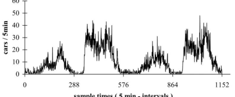
the boundaries of all comparable time series. Time series containing such trigger times are usually periodic but they can be aperiodic too, e.g. starting processes. Fig. 1 shows the periodic course of traffic flow, recorded by a measurement station.
0 10 20 30 40 50 60 0 288 576 864 1152
sample times ( 5 min - intervals )
cars /
5mi
n
Fig. 1. Periodic course of time of traffic flow over 4 days
For this example the time series can be subdivided in daily courses and the trigger points are fixed intuitive at 12.00am (points of time t0, t288, t576, t864 and t1152) of the
respective day. Figure 2 shows such a subdivision. However, the trigger points could be also at 4.20am and 8.20pm1. In this case, the period from 8.20pm to 4.00am is not
considered because it contains no relevant information for prediction.
The modelling method of fuzzy time series is based on finding subsets of similar time series in a set Z of single time series Zj. These subsets are called classes of time
series Zk (k=1,...,K) and they are generated by clustering techniques or generally
de-fined by experts with semantic contexts (workday, weekend, see figure 2). [1],[2],[5]
0 10 20 30 40 50 60 12:00 AM 4:00 AM 8:00 AM 12:00 PM 4:00 PM 8:00 PM 12:00 AM sample times cars / 5mi n Workday Holiday
Fig. 2. Sets of daily courses of traffic flow for two different types (classes)
Consequently, these classes contain representative time series, in which variations were tolerated.
The fuzzy pattern classification represents the possibility to convert such classes of time series into fuzzy descriptions in time. They reflect the representative courses of the classes. Additionally, they contain the deviations between the time series and various measurement errors as fuzziness. In some special cases the fuzzy prototypes can be defined only with expert knowledge.
2.2 Construction of the fuzzy time series model
Given are a set Z of time series and a class structure Zk ⊂Z. A class of time series Zk
consists from Nk courses of time Zj.
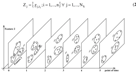
{
jt,}
kj z ;i 1,...,n j 1,...,N
Z = i = ∀ = (2)
All observations with the same index i are from same sample point ti. Consequently,
these sample points can be considered separately for construction of the fuzzy model. For every point of time, there are K several sets with Nk vectors
{
z,jt :j 1,...,Nk}
t,
k i = i =
Z ; k=1,...,K . (3)
These sets represent classes for the sample point ti and can be converted in a fuzzy
description Pk,tibased on the theory of fuzzy pattern classification [5].
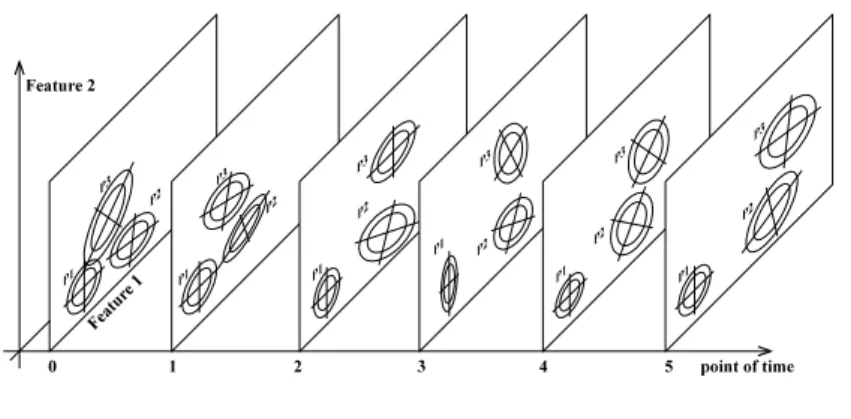
Fig. 4. Two-dimensional fuzzy time series model
As calculation results fuzzy classes Zk over ti lead to prototypes Pk
{
P :i 1,...,n}
Pk = k,ti = (4)
Fuzzy classes were described by multidimensional membership functions based on the potential function of Aizerman [1]. Vectors k
i t ; 0
P
z give the representatives of prototype and are included in fuzzy description by membership functions.
By using fuzzy model a sufficient data compression is realised. Simultaneously, errors (e.g. errors in measurement or rounding errors) can be inserted by the elementary fuzziness ce,m for every feature m of the model [6].
The construction of fuzzy prototypes from a set of time series is practicable by the program ZR_BUILD of the FX-Software-System [3].
3 Forecasting
3.1 The general attempt of forecasting
The precondition for time series prediction with fuzzy pattern classification is the fuzzy model. Furthermore, the incomplete time series being predicted must correspond to the model, i.e. context (measuring conditions etc.) and the sample points ti have to be the same. So the course can be assigned to one or several
representative prototype and it is forecasted by this classification, starting after the prediction point tV. That is the last known of time series. The forecasting of time
series by fuzzy methods is subdivided in two periods: the period of identification and the period of defuzzification.
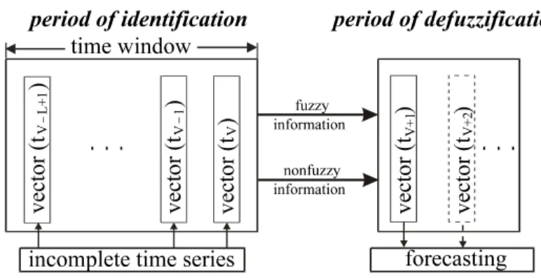
Fig. 6. Schematic description of the forecast by using fuzzy methods
The period of identification contains all algorithms for classification of time series to the prototypes. The classification of time series is done only in a time window with a length L. This time window contains the last sample times in the past, which will be used for identification of time series. The length of time window can be different for various times of prediction. The results of the period of identification are grades of membership to every prototype and vectors of position.
In the period of defuzzification the results of the period of identification will be transferred to the future for building new vectors of time series with algorithms as described in this paper. These new vectors represent the forecast of the corresponding time series.
In principle, there are two kinds of forecast: 1. global forecast
With the results of the period of identification at the time of prediction tV the time
series will be predicted for all points of times in the future. 2. recursive forecast
With the results of the identification by the time of prediction tV only the next
point of time tV+1 will be forecasted. Then the time tV+1 will be regarded as the
“new time of prediction” and the algorithm starts again.
3.2 The period of identification
In the period of identification the vector of grades of membership µ is calculated first. It describes fuzzy the position of the course of time which have to be forecasted. This vector consists of grades of membership for every prototype Pk.
The calculation of the grades of membership is carried out in the time window with length L. I.e., the feature vectors of the course must be identified for all sample times within the time window, which results in L different vectors of membership
(
P)
T i V t P i V t i V t − = µ1−,...,µ K− µ ; i = 1,...,L-1 . (5)They are obtained as follows:
{
0,...,L 1}
i ; 1 d c u 1 b 1 M 1 1 M 1 m P i V t , m P i V t , m P i V t , m P i V t , m P i V t k k k k k ∈ − − − + = µ∑
= − − − − − (6) where k i V P t −µ is the vector of membership to the prototype Pk for time tV-i.
The k k Pk i V t, m P i V t, m P i V t, m ,c ,d b − −
− are the fuzzy parameters of the corresponding prototype Pk for time tV-i and feature m. umPkt,V−i is the feature vector of the time series in the
class space [5].
The L different vectors
i V
t −
µ must be summarized to a resulting vector µ of membership with adequate methods. In this paper there will be used weighting functions or a fuzzy operation.
The weighting functions are defined in the time window as follows
( )
∑
∑
= = − + µ ⋅ = µ L 1 i i L 1 i P t i V P g g t k i L V k , (7)where µPk
( )
tV is the resulting grade of membership to the prototype Pk. The gi are
the weighting parameters for the points of time tV–L+i.
Here three weighting functions are used 1. arithmetical mean gi= 1 ; i = 1,...,L (8) 2. linear rising: gi= i ; i = 1,...,L (9) 3. exponential rising gi= ei ; i = 1,...,L (10)
Another kind of summarizing the grades of membership over the time with a fuzzy operation is based on the potential function of Aizerman. For that operation all points of time will be regarded equal.[6]
3.3 The period of defuzzification
The results of the period of identification are transferred to the period of defuzzification. Generally, the results are a vector of membership and information of position (nonfuzzy). These will be used for generating the new vector of the incomplete time series at the time tV+1 (recursive forecasting). In case of global
forecasting this data will be used for all remaining time points.
During forecasting, the grades of membership µPkare transferred to the sample time tV+1, i.e. the forecast vector zPtVk+1 must possess this grade of membership to the
corresponding prototype Pk.
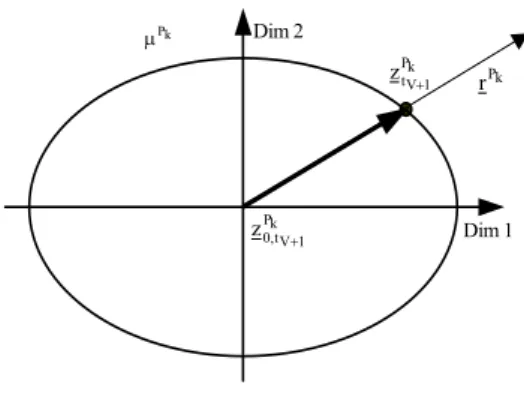
There is a set of feature vectors having this grade of membership of prototype for the time tV+1. This set is described by a hyperelliptic surface based on the potential
function of Aizerman (Figure 7).
By the nonfuzzy information of position exactly one feature vector can be selected out of this set. Generally, the information of position is a vector of direction rPk. This
vector is calculated at the time of prediction and describes the position of the vector of time series related to the representative vector k
1 V
P t, 0
z + of the corresponding prototype. It will be added to the representative vector for time tV+1 and there will be determined
Dim 2 k P µ k P r k P 1 V t , 0 z + k P 1 V t z + Dim 1
Fig. 7. Determination of the forecast vector
All of these vectors will be connected as follows
∑
∑
= = µ µ ⋅ = + + K 1 k P K 1 k P P t t k k k 1 V 1 V z z (11)The result is exactly one feature vector ztV+1. Simultaneously, it represents the prediction of the point of time tV+1. For the next step the point tV+1 is considered as the
new time of prediction and the algorithm starts again.
3.4 Implemented methods of forecasting
At present, there are three various kinds of forecast with fuzzy methods. In principle, the prediction algorithms are described in chapters 3.2 and 3.3., however for those three methods there are several extensions.
The first algorithm is called “forecasting by vector of direction”. This algorithm is exactly the method from chapter 3.2 and 3.3.
The second algorithm derives from the “forecasting by vector of direction”. This forecast algorithm is carried out for each feature, i.e. the multidimensional problem will be decomposed into several one-dimensional problems. For that reason it is called “method of one-dimensional forecasting”.
The third algorithm is named “method of the weighted gradients”. Unlike the two other methods, the gradients of the representative vectors are implemented for forecasting. A second classificator must be used for this method. It contains several prototypes of gradients which are connected to the prototypes of the time series2.
There is a prototype of time series for every prototype of gradients. The incomplete course of time will be classified to both prototypes and there emerge two grades of
2 Generally, the gradients of the course of prototype are equal to the representative vectors of
membership corresponding to every prototype of gradient. In the period of prediction these two grades will be combined by multiplication (based on the fuzzy AND-operation). The results are the weights for the gradients associated by the weighted average defuzzification method, i.e. the prediction consists of a vector of gradients continuing the incomplete time series up to the point of time tV+1.
3.5 Extensions of forecast for fuzzy methods
In this chapter several possibilities are suggested for extending the fuzzy methods of forecasting in a useful way and for eliminating errors of prediction. Usually, not all of the presented methods will be used for solving a problem.
1. Optimization of time windows
For all methods of forecast the length of time window at the time of prediction must be chosen. For the recursive methods that has to be done for all sample times. The length of time windows can influence the results of forecasting significantly. Particularly, for models of time series with several structures (e.g. crossed prototypes or stacked prototypes) it becomes enormously important. For a fuzzy model of time series, the time series for building these models can be implemented for optimizing the time window.
In order to achieve that, an error for every length of time window will be calculated for the corresponding sample time as a sum of forecasts. In principle, the time window with the minimum error will be used for prediction.
2. Rejection of time series
The potential function of Aizerman is defined in the whole feature space. Therefore, the possibility exists that prototypes with low grades of membership affect the forecast. Under the condition that there are many prototypes with this property the forecast could be wrong. Another example are crossed prototypes. At the time of crossing the influence of a “false” prototype is getting higher , i.e. the grade of membership is increasing. Generally, the prediction after this time could be wrong3. In these cases, the incomplete time series can be rejected by
prototypes within the time window at time of prediction. Consequently, the grades of membership are set to zero for the remaining time.
3. Masking of prototypes
For solving problems it could be useful to create several fuzzy models of time series based on certain verified supplementary conditions. Generally, this method extension results in a better description of the reality. Especially, the mutual influence of prototypes without context can be avoided. The supplementary conditions are mostly nonfuzzy information like season4,
weekday, type of machine or kind of production. The incomplete time series is
3 This effect will be preferred by several models. Therefore the rejection of time series depends
on specified problems.
classified to one of the models according such a condition5 and thus makes
possible sophisticated forecast. 4. Additional features
For some problems it is useful to possess further forecasting information. This information could be available in form of values of features, which are not going to be forecasted. In principle, the problem can be divided in two parts: the fuzzy model of time series and the further fuzzy model “of correction”. Similar to the algorithm of prediction from the original model, the model of correction generates a feature vector of offsets which have to be added to the results of prediction at the sample time tV+1. Only at this time offsets are added. Examples
for such features are brightness and temperature at forecast load curves of power or numbers of cars for forecasting the demand of replacement parts.
4 Examples of Projects
In the following several projects processed at the Professorship of System Theory will be introduced.
4.1 Analysis of traffic density
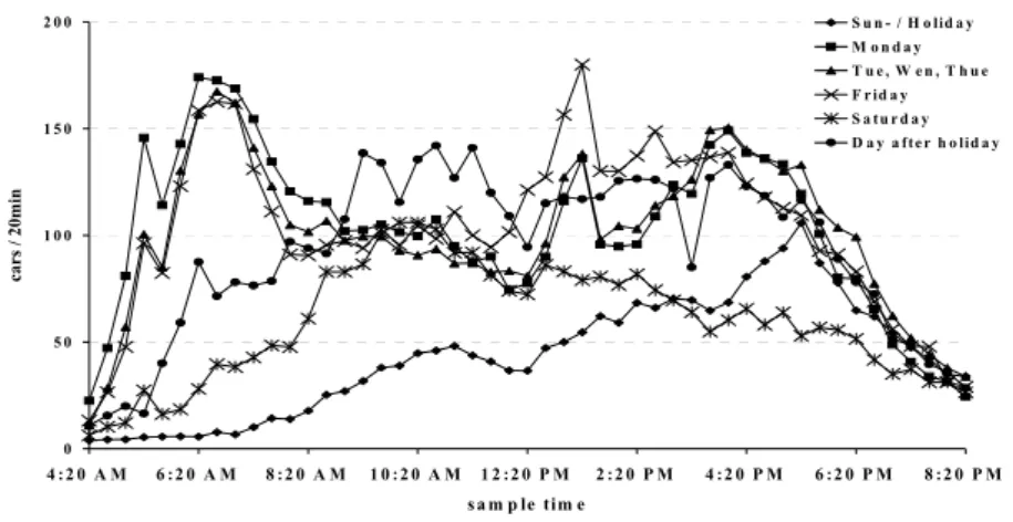
Analysis and forecasting of traffic flow was the topic of the dissertation of Warg [8]. At a federal road traffic flows have been measured over several weeks (fixed measurement position). The trigger points were set at 4.20am and 8.20pm.
0 5 0 1 0 0 1 5 0 2 0 0 4 :2 0 A M 6 :2 0 A M 8 :2 0 A M 1 0 :2 0 A M 1 2 :2 0 P M 2 :2 0 P M 4 :2 0 P M 6 :2 0 P M 8 :2 0 P M s a m p le tim e cars / 20min S u n - / H o lid a y M o n d a y T u e , W e n , T h u e F r id a y S a tu r d a y D a y a fte r h o lid a y
Fig. 8. Fuzzy model of traffic flows; The meanings of the prototypes are shown in the legend.
5 It is conceivable, that more than one of the models can be selected according to conditions.
The model of time series could be considered as different time slot patterns. Here only a time pattern of 20 minutes is presented. Furthermore, the classes of time series were built based on semantic information. Figure 8 shows the corresponding fuzzy model. The forecast of incomplete traffic flows leads to very good results. Three random selected traffic flows are shown in the following figure. The time of prediction was at 6.20am and forecasts were calculated to the end of time of the model (8.20pm). The method of weighted gradients was used.
As it shows, the forecasted courses of time describe the original courses of the corresponding time series very well.
0 20 40 60 80 100 120 140 160 180 200 4:20 AM 6:20 AM 8:20 AM 10:20 AM 12:20 PM 2:20 PM 4:20 PM 6:20 PM 8:20 PM sample time cars / 20 min Tuesday Forecasted Tuesday Thursday Forecasted Thursday Sunday Forecasted Sunday
Fig. 9. Forecast of traffic flows; At several sample times the forecasted course does not
corres-pond to the original course. E.g. at 1.00pm and 1.20pm there does not exist top for the Tuesday course such as in the model. That is not foreseeable and errors of forecasting are very high.
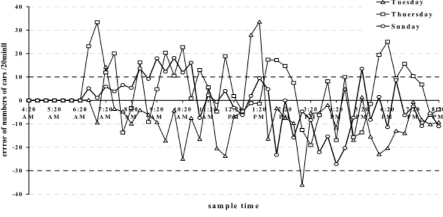
-4 0 -3 0 -2 0 -1 0 0 1 0 2 0 3 0 4 0 4 :2 0 A M 5 :2 0A M 6 :2 0A M 7 :2 0A M 8 :2 0A M 9 :2 0A M 1 0 :2 0A M 1 1 :2 0A M 1 2 :2 0P M 1 :2 0P M 2 :2 0P M 3 :2 0P M 4 :2 0P M 5 :2 0P M 6 :2 0P M 7 :2 0P M 8 :2 0P M s a m p le tim e errror of numbers of cars /20minll T u e s d a y T h u e r s d a y S u n d a y
Fig. 10. Forecasting errors of traffic flow; It can be noticed, that the forecasting errors do not
4.2 Forecasting of load curves
The assignment of this study was the implementation of a forecast method for load curves of energy [9]. There were 100 daily load curves at disposition. Naturally, the trigger points were at 12.00am. Two days had to be rejected because they had too much measuring faults. All other faults could be recovered by linear regression.6
Four fuzzy models of time series were built by masking the prototypes7. The
supplementary condition was the date of the days. By this date the periods of summer and winter time and furthermore the workdays and the holidays are distinguished.
marking time series
evaluation period
summer time winter time
evaluation weekday
workday holiday workday holiday
evaluation weekday model summer workday 11 TS; 2P model summer holiday 5 TS; 2P model winter workday 57 TS; 8P model winter holiday 23 TS; 4P P R E D I C T I O N
Fig. 11. Allocation of time series for several models by dates; In this figure there are shown
the numbers of time series (TS) which built the models and the numbers of corresponding prototypes (P). Incomplete time series are at first assigned to one model and the forecasting is calculated within the model.
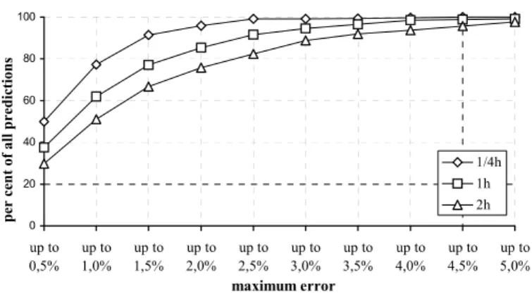
The forecast of the load curves must fulfill the following restriction: The errors of prediction of the next point of time (15min) must be lower than 3% of the original value at 98% of all forecasts. Figure 12 shows the results for the “workday-winter time” model for 7 daily courses, which were not used for building the prototypes. In addition, there are shown the forecasting results for one and two hours.
6 There were maximal two faults in turns. 7 See also chapter 3.5
0 20 40 60 80 100 up to 0,5% up to 1,0% up to 1,5% up to 2,0% up to 2,5% up to 3,0% up to 3,5% up to 4,0% up to 4,5% up to 5,0% maximum error
per cent of all predictions
1/4h 1h 2h
Fig. 12. Error distribution for the model of load curves (workday – winter time) – by 7 time
series; The numerical values of the errors up to 3% are 99.26% for the 1/4h, 94.49% for the 1h and 88.84% for the 2h prediction.
The table 1 shows the quality of prediction of all time series with the condition “workday – winter time ”. The error distribution is nearly the same as in figure 12. For all other models the results are similar.
1/4h 1h 2h up to 0,5 % 54,53 % 41,31 % 32,37 % up to 1,0 % 82,09 % 68,35 % 56,80 % up to 1,5 % 92,70 % 82,28 % 72,35 % up to 2,0 % 96,71 % 89,43 % 82,01 % up to 2,5 % 98,40 % 93,45 % 87,74 % up to 3,0 % 99,05 % 95,59 % 91,56 % up to 3,5 % 99,42 % 97,01 % 93,86 % up to 4,0 % 99,70 % 98,13 % 95,39 % up to 4,5 % 99,82 % 98,68 % 96,48 % up to 5,0 % 99,91 % 99,08 % 97,40 %
Table 1. Error distribution of the model of load curves (workday – winter time)
4.3 Analysis and prediction of ecological data
The task of the project “Time series analysis and prediction of ecological data” [8] was to transfer that ecological data of sewage works in a fuzzy model of time series and to test this model for forecasts of up to 10 hours. There were 5 different measurement variables. In this paper only the “pH-value” will be discussed.
The time series consist of daily courses of 96 measurement values (15min intervals). Altogether, there were 69 time series for building the model. The first step
was the clustering of time series. After evaluation by experts from the 8 emerged classes only 4 prototypes remained (Figure 13).
0 0,2 0,4 0,6 0,8 1 1,2 1 6 11 16 21 26 31 36 41 46 51 56 61 66 71 76 81 86 91 96
sample time (15min)
pH-val ue ( normed) prototype 1 prototype 2 prototype 3 prototype 4
Fig. 13. Fuzzy model of time series of pH-values (daily courses)
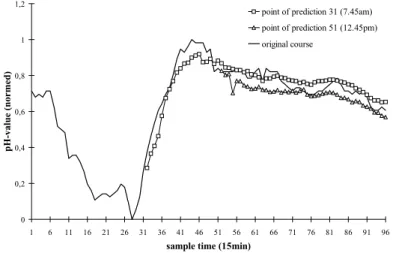
For forecasting of incomplete courses of pH-values the results are good. The prediction up to 10 hours has a middle relative error at about 10%. The next figure shows the forecast of one time series from 7.45am and another from 12.45pm.
0 0,2 0,4 0,6 0,8 1 1,2 1 6 11 16 21 26 31 36 41 46 51 56 61 66 71 76 81 86 91 96
sample time (15min)
pH-va lue ( n or me d)
point of prediction 31 (7.45am) point of prediction 51 (12.45pm) original course
Fig. 14. Examples for the forecasting of ecological time series (pH-value); The middle relative
References
1. Bock, H.H.: Automatische Klassifikation, Vandenhoeck & Ruprecht, Göttingen 1974 2. Bocklisch, S. F.: Prozeßanalyse mit unscharfen Verfahren, Verlag Technik Berlin (1987) 3. FX-System, Nutzerhandbuch, TU Chemnitz, Professur für Systemtheorie (1999) 4. Harvey, A. C.: Zeitreihenmodelle, R. Oldenburg Verlag, München Wien (1995)
5. Päßler, M.: Automatische Klassifikation, Praktikumsarbeit, TU Chemnitz, Professur für Systemtheorie (1995)
6. Päßler, M.: Mehrdimensionale Zeitreihenanalyse und -prognose mittels Fuzzy Pattern Klassifikation, Diplomarbeit, TU Chemnitz, Professur für Systemtheorie (1998)
7. Päßler, M.: Zeitreihenanalyse und -prognose mittels Fuzzy Pattern Klassifikation, Information 06/99, TU Chemnitz, Professur für Systemtheorie
8. Bocklisch, Buchholz, Lindner, Stephan: Zeitreihenanalyse und -prognose umweltrelevan-ter Meßverläufe, Information 05/99, TU Chemnitz, Professur für Systemtheorie (1999) 9. Kurzbeschreibung der Zeitreihenanalyse und -prognose mittels Fuzzy Pattern
Klassifika-tion für die Problematik der Energielast- und -bezugsprognose, TU Chemnitz, Professur für Systemtheorie (1998)
10. Warg, S.: Verkehrsstromanalyse und -prognose mit Fuzzy Pattern Klassifikation, Diplomarbeit, TU Chemnitz, Professur für Systemtheorie (1997)