Technology differences, institutions and economic growth : a conditional conditional convergence

Technology differences, institutions and economic

growth : a conditional conditional convergence

_____________

Hervé Boulhol

growth : a conditional conditional convergence

_____________

Hervé Boulhol

No 2004 – 02

February

3 TABLE OF CONTENTS SUMMARY...4 ABSTRACT...5 RÉSUMÉ...6 RÉSUMÉ COURT...7 1. INTRODUCTION...8

2. TECHNOLOGY DIFFERENCES AND DIFFUSION...10

3. GROWTH EQUATIONS AND INSTITUTIONS...11

4. DATA...13

5. FROM THE INSTITUTIONAL DATABASE TO THE ECONOMETRIC SPECIFICATION...15

6. RESULTS...17 7. CONCLUSION...24 BIBLIOGRAPHY...25 APPENDIX 1...38 APPENDIX 2...41 APPENDIX 3...45 APPENDIX 4...46

TECHNOLOGY DIFFERENCES

,

:

SUMMARY

The augmented Solow model by Mankiw, Romer and Weil (1992) exhibited the role of human capital for long term growth path and led its authors to accept either the assumption of identical technology across countries or the treatment of technology differences as residuals in the growth equation. However, Hall and Jones (1996, 1999) and Klenow and Rodriguez-Clare (1997) have shown that productivity levels and output per worker are highly correlated, which casts doubts on the conditional convergence scenario. Yet the cross section literature has not drawn the necessary implications. Acknowledging the importance of taking into account productivity differences, we break down productivity into two components: a pure technological part and its complement called “efficiency”. From a simple model of technology diffusion, we focus on the interactions between institutions and technology differences and identify three complementary channels through which institutions impact growth: efficiency in the use of technology, long term TFP-growth and technology diffusion.

To shed light on how growth and institutions interplay, our framework is tested from a new and detailed database on institutions developed by the French Ministry of Economy, Finance and Industry (MINEFI). Data was collected through a questionnaire by the Economic Missions of the MINEFI in 51 countries representing 80% of world GDP. The database consists of 330 items on institutions in a broad sense, each receiving a ranking from 0 to 4 for each country. The robustness of the database has been established by Berthelier, Desdoigts and Ould-Aoudia (2003) through a comparative study with other institutional databases used in various economic studies.

We find that technology diffusion substantially impacts economic performance and that catching-up is conditional to the quality of the appropriate institution – a mix of R&D, innovation and capital-risk support -, with the annual rate of convergence to the technological frontier varying from 0% to 12.4% depending on the country . Institutions also matter for technological efficiency, as our non-corruption variable, for instance, contributes as much as the stock of human capital to the productivity level heterogeneity. Moreover, long run TFP-growth differences are significantly determined by such institutions like the ones reflecting a competitive product market or a favourable innovation environment. Having controlled for institutions, international trade measured, by the openness rate, is insignificant to explain neither TFP-growth differences nor technology diffusion. However, when we take the manufacturing share in exports into account, we find a significant impact of trade on TFP-growth, coming solely from the richer countries in the sample, which clearly points to a non-linearity. This suggests that the contribution of trade is positive only if the specialisation is appropriate and the development fairly advanced. This last result is tentative because of potential endogeneity biases. Including human capital flows as a determinant of the steady-state reveals that MRW’s approach and ours are

5

complements rather than substitutes. Conditional convergence here is also conditional to sharing the same technology and quality of institutions, which renders recent observed divergence well accounted for.

ABSTRACT

Highlighting that technology is only a component of productivity, this study focuses on the interactions between institutions and technology differences to explain cross-country growth pattern. Three complementary channels through which institutions impact growth are identified: efficiency in the use of technology, long term TFP-growth and technology diffusion. From a new and detailed database on institutions developed by the French Ministry of Economy, Finance and Industry, poor institutional quality, beyond human capital, is estimated to be the source of an annual growth-rate loss of between 2.4 and 6.1 percentage point for half of the countries. Technology diffusion speed is institutionally related and the distance to the technology frontier is reduced from 0% to 12.4% annually depending on the country. Trade has a non linear influence on growth, being significant only for countries already advanced in the development phase. Conditional convergence here is also conditional to sharing the same technology and quality of institutions, rendering recent observed divergence well accounted for.

J.E.L. classification: O11; O33; O47

ECARTS TECHNOLOGIQUES

,

:

RÉSUMÉ

L’extension du modèle de Solow par Mankiw, Romer et Weil (1992) a mis en évidence le rôle du capital humain pour le sentier de croissance à long terme et a conduit ses auteurs à accepter l’hypothèse d’une technologie identique pour l’ensemble des pays ou le traitement des différences technologiques comme résidus des équations de croissance. Hall et Jones (1996, 1999) et Klenow et Rodriguez-Clare (1997) ont cependant montré que les niveaux de productivité et de production par tête étaient fortement corrélés, remettant en cause le scenario de convergence conditionnelle, sans que la littérature en ait tiré toutes les implications qui s’imposent. Reconnaissant l’enjeu de la prise en compte des différences de productivité, nous décomposons la productivité en deux éléments : une composante purement technologique et son complément que nous appelons « efficacité ». A partir d’un modèle simple de diffusion technologique, nous nous concentrons sur les interactions entre les institutions et les différences de technologies pour expliquer l’évolution comparée de la croissance entre pays. Trois canaux complémentaires par lesquels les institutions ont une influence sur la croissance sont identifiés: l’efficacité dans l’utilisation des technologies, la croissance de la productivité à long terme et la diffusion des technologies.

Pour clarifier les interactions entre les institutions et la croissance économique, notre modèle est testé à partir d’une nouvelle base de données institutionnelles détaillée, développée par le MINEFI. Les données ont été collectées par les Missions Economiques du MINEFI dans 51 pays représentant 80% du PIB mondial. La base de donnée est composée de 330 items sur les institutions, notion prise dans son sens large, chacun d’entre eux recevant une note entre 0 et 4 pour chaque pays. Berthelier, Desdoigts et Ould-Aoudia (2003) ont établi la robustesse de la base en la rapprochant d’autres bases de données institutionnelles utilisées dans les travaux économiques.

Nous trouvons que la diffusion technologique a un impact substantiel sur la performance économique et que le rattrapage est conditionnelle à la qualité de l’institution adéquate – un mélange de R&D, d’innovation et de support au capital-risque -, avec une vitesse annuelle de convergence vers la frontière technologique variant de 0% à 12,4% selon les pays. Les institutions importent aussi pour l’efficacité dans l’utilisation des technologies, et notre mesure de la non-corruption, par exemple, contribue autant que le stock de capital humain à la dispersion de la productivité. De plus, les différences de croissance de la productivité totale des facteurs (PTF) à long terme sont significativement déterminées par des institutions telles que celles reflétant un marché des produits concurrentiel ou un environnement favorable à l’innovation. En contrôlant les différences institutionnelles, le commerce international, mesuré par le taux d’ouverture, n’est significatif ni pour expliquer les différences de croissance de la PTF ni pour la diffusion des technologies. Cependant, lorsque l’on prend en compte la part des biens manufacturés dans les exportations, alors nous trouvons un impact significatif du commerce sur la croissance de la PTF, provenant

7

seulement des pays les plus riches dans l’échantillon, ce qui indique une non-linéarité. Cela suggère que la contribution du commerce est positive seulement si la spécialisation est appropriée et le développement déjà avancé. Ce dernier résultat est fragile en raison d’éventuels biais d’endogénéité. De plus, la prise en compte de l’impact du flux de capital humain pour l’état régulier révèle que l’approche de MRW et la notre sont des compléments plutôt que des substituts. La convergence conditionnelle est ici conditionnelle aussi au fait de disposer des mêmes technologies et des mêmes institutions, et rend compte de la divergence récemment observée.

RÉSUMÉ COURT

Insistant sur la distinction entre productivité et technologie, cette étude se concentre sur les interactions entre les institutions et les écarts de technologiques pour expliquer l’évolution comparée de la croissance entre pays. Trois canaux complémentaires par lesquels les institutions ont une influence sur la croissance sont identifiés: l’efficacité dans l’utilisation des technologies, la croissance de la productivité à long terme et la diffusion des technologies. A partir d’une nouvelle base de données institutionnelles détaillée, développée par le MINEFI, nous estimons que l’insuffisante qualité des institutions, au-delà du capital humain, est la cause d’un déficit de taux de croissance annuelle entre 2,4 et 6,1 point de pourcentage pour la moitié des pays. La vitesse annuelle de diffusion des technologies varie de 0% à 12,4% selon les pays en fonction de leur niveau institutionnel. Le commerce a un impact non linéaire sur la croissance puisqu’il est significatif seulement pour les pays déjà avancés dans la phase de développement. La convergence conditionnelle est ici conditionnelle aussi au fait de disposer des mêmes technologies et de la même qualité des institutions, et rend compte de la divergence récemment observée.

J.E.L. classification: O11 ; O33 ; O47

TECHNOLOGY DIFFERENCES

,

:

Hervé Boulhol

1.

The seminal article by Mankiw, Romer and Weil (1992), subsequently denoted MRW, shed light on the contribution of human capital in reconciling the measured low speed of conditional convergence between countries with a physical capital share of around one-third. Their main conclusion is that, when human capital is added, the then augmented Solow model is well suited to analyse growth across countries. It follows that, contrary to endogenous growth theory, the growth process is solely driven by factor accumulation (including human capital), is consistent with a rate of convergence of around 2% a year (rather than the 4%-5% expected from the Solow textbook model) and validates underlying assumptions of constant returns to scale and identical technology. The MRW framework has been criticised on different grounds. First, the embedded human capital theory treats human capital just as another accumulating factor. This implies that human capital should enter into growth equation through its growth rate, but there is confusion in whether the stock of human capital matters rather than the flow as in MRW. Benhabib and Spiegel (1994) convincingly support the view that the stock of human capital is a “determinant of the magnitude of a country’s Solow residual”. Second, as most of the cross-country literature, the MRW approach is subject to the bias coming from the identical technology assumption.

The conditional convergence predictions has been more and more difficult to reconcile with the facts pointing to global divergence as outlined by Pritchett (1997). Prompted by J.Temple’s fourth question about the causes of income differences (Temple, 1999, p.113), we start from the inference that if poor countries are poor not only because of a lack of inputs that will accumulate faster fostering convergence, it must be that they are poor also because of overall efficiency and technology differentials - whatever these mean - that may persist or aggravate over time especially if they are due to institutional differences.1 The role of institutions as a determinant of long term growth is increasingly recognised, yet more research is needed to disentangle which institutions matter for economic performance and above all to incorporate them properly in economic theory. Even though Rodrik (2002, 2003) is convincing in arguing that the same institutions may have different economic

(*): I would like to express my gratitude to Lionel Fontagné, Jacques Ould-Aoudia and Patrick Artus for having made this study possible. I would particularly like to thank Agnès Bénassy-Quéré, Guillaume Gaulier, Romain Rancière and the participants of the Cepii seminar for their valuable comments. Finally I very much appreciated the help I received from Maylis Coupet and David Galvin, as well as the warm welcome I received from Cepii employees.

1

9

impacts based on a country’s idiosyncrasies, we suggest that the quality of some institutions does influence economic performance overall. In this study, we show that technology differences play an important role in the cross-country growth pattern and that institutions matter for total factor productivity (TFP) level and growth rates, and for technology diffusion.

Many reasons may explain why technology differs significantly between countries. Patent protection, learning by doing, knowledge differences detract technology from its public-good pretension (Caselli, Esquivel and Lefort, 1996). Moreover, taking a broader view of productivity, institutions linked to the social, political or legal aspects of efficiency contribute to productivity differentials. Surprisingly, the growth literature does not pay enough attention to heterogeneity in technology. When it does, this heterogeneity is treated in panel estimates and as a fixed effect, the details of which are rarely available, making an assessment of whether they do represent what they should difficult. Exceptions are Hall and Jones (1996, 1999), Klenow and Rodriguez-Clare (1997) who precisely estimate productivity differences and Bloom, Canning and Sevilla (2002) whose concerns are close to ours. We hope our contribution to be theoretical and empirical. Theoretically we identify three channels through which institutions may impact productivity. First, a static contribution through efficiency in the use of technology, second a persistent dynamic one through long run TFP-growth rates and third a temporary dynamic one through technology diffusion. Empirically we test our framework using a new and detailed database on institutions that was developed by the French Ministry of Economy, Finance and Industry (MINEFI). Data from a questionnaire was collected by the Economic Missions of the MINEFI in 51 countries representing 80% of world GDP. The database consists of 330 items on institutions in a broad sense, each receiving a ranking from 0 to 4 for each country. We find that technology diffusion substantially impacts economic performance and that catching-up is conditional to the quality of the appropriate institution – a mix of R&D, innovation and capital-risk support -, with the annual rate of convergence to the technological frontier varying from 0% to 12.4% depending on the country . Institutions also matter for technological efficiency, as our non-corruption variable, for instance, contributes as much as the stock of human capital to the productivity level heterogeneity. Moreover, long run TFP-growth differences are significantly determined by such institutions like the ones reflecting a competitive product market or a favourable innovation environment. In addition, including human capital flows as a determinant of the steady-state reveals that MRW’s approach and ours are complements rather than substitutes. Having controlled for institutions, international trade measured, by the openness rate, has a non-linear contribution to TFP-growth, being significant and positive only if the specialisation is appropriate and the development fairly advanced. This last result is tentative because of potential endogeneity biases.

The study is organised as follows. Section 2 highlights the importance of taking into account technology differences and introduces our approach regarding the technological process. Section 3 details how institutions and growth interplay in the model. Section 4 describes the data and the selection of the institutional variables, leading to the econometric

specification in Section 5. Results are presented in Section 6 where econometric issues are also discussed. Finally, Section 7 concludes.

2.

The most disputable critical assumption in the cross-section growth literature suggests that either all countries share the same level of technology and technological progress or that the differences in these levels are treated as residuals, implying that they are being considered independent from other explanatory variables. This is an extreme conjecture since it means that technological change spreads instantaneously and completely to every country, whatever the level of openness or institutional profile, and leads to having only the differences of capital per unit of labour to explain differences of output per capita. Assuming a Cobb-Douglas production function and with standard notations,

b a i i b i a i i K H AL Y = . ( )1− − (1)

where Y is output, K and H are stocks of physical and human capital respectively, A is the productivity level and L the number of workers. Output per worker y_i for the country i is therefore given by a i KH i b a i b i i a i i b a i i i i Y L A K L H L A Z L y ≡ / = 1− − .( / ) .( / ) ≡ 1− − .( / ) (2)

with ZKH =K.(H/L)b/a defining a capital aggregate built from the physical capital stock and the human capital stock per capita. If we assume that the productivity level A_i is independent of the country (Ai =A,∀i), then the ratio of output per capita in 1980 between the USA and Uganda of 48 to 1, being the two extremes in our data, translates into a highly unrealistic capital aggregate, ZKH, per capita ratio of 110,700 to 1 using a physical capital share of one-third. Moreover, recognising the productivity differences, it is apparent from equation (2), valid at each time,that both the initial productivity level and the initial output per capita are closely linked, which renders growth equation estimates assuming identical productivity seriously biased. While this inconvenience is well-acknowledged, the growth literature has not drawn yet all the necessary implications. Over the last fifteen tears, economic research has made some notable advances in the understanding of what productivity is. However, the essence of its contents remains unknown, and the parameter A is often indistinctly designated as either the productivity or the technology level. This creates confusion in identifying the role of technology and therefore, adopting a different posture, we insist here on the distinction between the two notions and call the complement of technology in productivity: “efficiency”. Inspired by Bassanini and Scarpetta (2001), we break down the total level of productivity A_i into two components: a pure technology level B_i and the degree of efficiency in using this technology X_i so that A_i equals B_i.X_i. As the benchmark, the country with the highest GDP per capita in 1980, the USA, has been chosen. We denote b_i =B_i /B_ben, an inverse

11

indicator of the distance to the frontier, x_i =X_i/X_ben , the ratio of the relative efficiency to the benchmark, and a_i = A_i /A_ben=b_i.x_i, the relative productivity level. Institutional quality is considered as impacting the technological efficiency X_i and possibly the technology diffusion which process is most simply governed by:2

)) ( 1 .( ) (t v b t b&_i = _i − _i (3)

where t stands for time: in the long run technologies converge to the frontier at a pace represented by v_i, which will be tested as being constant across countries or institutionally-related. Note it is only the pure technology component that is assumed to converge (or diverge if v_i is negative), and total productivity discrepancies may persist as a result of differences in institutionally-related efficiency X_i.

3.

We suppose that institutions enter into growth equations through three different channels: the level of technological efficiency, the progress of technological efficiency and possibly the speed of technology diffusion. Noticing that the productivity level A_i can be written as

i i ben x b

A . . , we can split TFP-growth into three components:

i i i i ben ben i i b b x x A A A

A& & & &

+ +

= (4)

The first term on the right is simply the benchmark TFP-growth, denoted by g, the second, denoted −c_i, is the long run TFP-growth deficit to the benchmark and the third is the technological catch-up component derived from resolving the differential equation (3).

)) 0 ( 1 ( )) 0 ( 1 .( . i t v i i i i i b e b v c g A A i − − − + − = & (5)

Institutions will have an impact through Xi(0), through ci, and potentially through vi.

We now need to integrate equation (5) into the growth equation. The growth model we then develop is the augmented Solow model enriched to take into account the heterogeneity of technologies and the contribution of institutions. With n_i denoting the population growth, d the physical and human capital depreciation rate, s_iK and s_iH the fraction of total income invested in physical and human capital respectively, Appendix 1 establishes the following growth equation:

2

In a recent paper, Benhabib and Spiegel (2003) refers to this diffusion process, originating in the Nelson-Phelps model, as the confined exponential diffusion process.

)) 0 ( ( ) ( ) .( ) ( . 1 ) 0 ( ). 0 ( ) 0 ( . 1 ) 0 ( ) ( , ) 1 /( 1 . . i t v i b a b a i i b H i a K i t ben i i t i i b f c g c g d n s s Log t e A a y Log t e t y Log t y Log i i + − +         − + + − + − − = − −− + − −β β (6)

where βi =(1−a−b).(ni+d+g−ci) is the usual speed of conditional convergence and

the last term

            − ≈ − − = − i i i t v i i t v v b b e b Log t b f i . 1 ) 0 ( 1 ) 0 ( )). 0 ( 1 ( 1 . 1 )) 0 ( ( . , (7)

is the contribution of technology diffusion to growth: it is positively related to the speed v_i and to the distance to the technological frontier. Equation (6) is to be compared to the augmented-Solow growth equation which is exactly the same as if we assume that initial total productivity level A_i(0) is identical across countries, that every country is at the frontier (bi =1)and that there is no long term TFP-growth differences (ci =0). The

growth process is therefore the result of four distinct forces: the “adjusted” absolute convergence – this source of convergence is lessened here because of overall productivity level differences, therefrom the adjective “adjusted” -, a second convergence component coming from technological catch-up, the usual non-convergence stemming from differences in long term paths due to different investment rates and an additional divergence force coming from long term TFP-growth differences.

The main reason for considering that all countries share the same technology lies in the difficulty to observe relative technology levels. What is only needed here, as shown by equation (6), is the relative level of initial productivity and there is one piece of information from which we can estimate it. Indeed equation (2) illustrates that initial output per worker is certainly linked to initial productivity. We will assume that a part η of initial income ratios can be explained by initial productivity ratios, the complement 1−η being explained by capital differences, and therefore we formally write:

η       = ≡ ) 0 ( ) 0 ( ) 0 ( ) 0 ( ) 0 ( ben i ben i i y y A A a (8a)

Hence η is characterised by:

)) 0 ( ( )) 0 ( ), 0 ( ( i i i y Log Var y Log a Log Cov = η (8b)

Klenow and Rodriguez-Clare (1997) use estimates of stocks of physical and human capital to infer productivity levels and assess that “productivity differences account for half or more of level differences in 1985 GDP per worker” (p.75). For instance according to

13

equation (2), with η=0.75 and a =b=1/3, the output per capita ratio between the USA and Uganda of 48 in 1980 is “explained” by a contribution from the productivity level ratio of 2.7 and a capital aggregate, ZKH, per capita ratio of 6,100 instead of 110,700. For sure, the extreme simplification in equation (8a), which has though the merit of highlighting the potential correlation between initial productivity and initial output per worker, and of avoiding the main pitfall of the cross-section approach, is a strong ad hoc assumption, but taking η=0, as is done in most of the cross-section literature, is as strong and certainly a far more inaccurate ad hoc assumption.

4.

4.1.

General data

The time frame is the period from 1980 to 2000. For data entering the traditional Solow model, we use Penn World Table 6.1.3 The per capita output is the real GDP per capita at Purchasing Power Parity, chain series. For the investment rate s_iK, we use the average over the period of the investment share of real GDP (variable ki in the database). As in MRW, the proxy for the rate of human capital accumulation is the percentage of the working-age population in second-level education. This percentage is constructed by multiplying the gross secondary enrollment rate (World Development Indicators) by the percentage of the working-aged population aged 15 to 19. The average of this variable over the years 1980, 1990 and 2000 is named HCFLOW.

4.2.

Institutions database

We use an original database on institutions developed by the MINEFI, well described and analysed in Berthelier, Desdoigts and Ould-Aoudia (2003). This database focuses primarily on emerging countries as 44 of the 51 countries are developing countries and also includes a control group of developed countries. Data was gathered from a very detailed questionnaire: for each country, 330 items aggregated in 115 indicators were made available. As an example the indicator related to the efficiency of public policy linked to the quality of the tax system is built from four items assessing the importance of the black market, the importance of fraud in the formal economy, in customs and the capacity of the Administration to implement tax measures. Importantly, Berthelier et al have established the robustness of the database by highlighting its convergence with various institutional databases (World Bank, Fraser Institute, Economist Intelligence Unit, Political Economic Risk Consultancy, IMF, Transparency International among others) all covering 30% of the stock variables from the questionnaire. The limitations of the database are twofold: a fairly small number of countries and a time period limited to a single point in or close to year 2000. We will consider that the institutional profile for a given country is stable over the

3

Alan Heston, Robert Summers and Bettina Aten, Penn World Table Version 6.1, Center for International Comparisons at the University of Pennsylvania (CICUP), October 2002.

period of the growth analysis. This raises poisonous questions of endogeneity since a country experiencing a favourable economic development increases its chances of developing better institutions and the causality between growth and institutions might be reversed. Therefore, those indicators that are too suspicious in this respect are excluded and this endogeneity issue is econometrically addressed in section 6.4.

For the purpose of the study, we cluster the remaining 94 indicators into five groups representing distinct aspects of the institutional profile. These five institutional domains cover product market, labour market, financial system, innovation and a general heading for all other indicators. Each domain is analysed through a factor analysis which aggregates the original indicators and provides robust institutional variables synthesising most of the information in the database.

4.3.

Factor Analysis

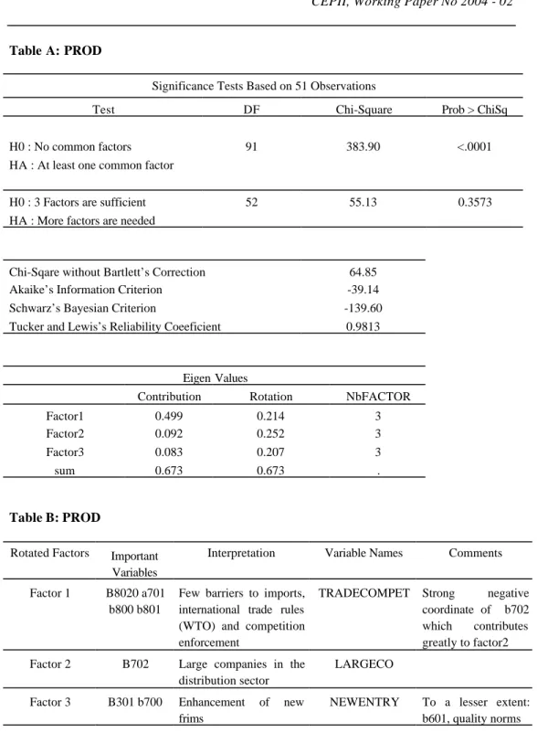
The chosen approach is very close to that of Nicoletti, Scarpetta and Boylaud (1999) developed to build product market regulation indicators. It differs only in the factors aggregation methodology and details are found in Appendix 2. The idea is simple: for each domain, we run a factor analysis and select the number of relevant factors according to usual tests. The axes are then rotated in order to enhance interpretation of factors and an aggregated index is built for each domain. Unsurprisingly these aggregated indices are extremely correlated with each other so that valuable detailed information is lost in the aggregation process. As a consequence we preferred to use, as explanatory variables for the role of institutions on growth, the factors that contained enough information and were easily identified. Therefore we will focus on variables which retain more than 25% of their domain variance. Table 1 summarises the variables which passed these tests.4 In addition to the aggregated indices, five other variables are selected: CORRUPTION, an indicator of the non-corruption level, CONTRACT, a variable referring to the contractual importance in the labour market, BANKRULES, assessing the quality of bank regulation and prudential rules, R&D-CAPRISK, an indicator of R&D/innovation effort and favourable capital risk system and INTPROP, a variable linked to the protection of intellectual property rights (IPRs).5 If we lower our threshold to 20% of the variance, three of the six then added variables are of particular interest since they represent a very distinct aspect of the product market institutions: TRADECOMPET, an indicator of the international and domestic pro-competitive environment, LARGECO, the share of large companies in the distribution sector, which may be an indicator of efficient scale, and NEWENTRY, representing low barriers to new entry. Charts 1 and 2 represent the countries in a two-dimensional plan for the institutional variables that will be of particular interest below: CORRUPTION, R&D-CAPRISK and PRODINDEX. Chart 1, for instance, indicates a strong positive correlation

4

As always with factor analysis, the advantage of such a methodology is that the final indicators are computed as objectively as possible based on the data. The main inconvenience is almost identical. Indicators are data based which means that they depend upon the specific sample and if we add new countries, indicators for countries in the original sample will be altered.

5

For the labour market and financial system domains, because the general index is fairly intangible, the factors only will be used (see Appendix 2, $ 3.3 and 3.4).

15

between the non-corruption variable and the initial GDP per capita, but also shows that the corruption index adds valuable information, as a given GDP per capita level may be associated with a wide range of corruption levels.

< Table I, Charts 1 and 2 >

5.

5.1.

Institutional variables

The indicators in Table 1 are the candidates for the computation of our institutional variables. These indicators are indifferent to a linear transformation and we linearly normalise them so that they meet the constraints embedded in the model presented in sections 2 and 3 as follows. We define Ic,IX(0),Idiff the institutional indicators that are respectively linked to long term TFP-growth, initial efficiency in the use of technology and technology diffusion. As by definition c_ben equals 0, the long term TFP-growth deficit to the benchmark, c_i, is defined by:

) .( _benc _ic

i c I I

c = − (INST 1) where c is a parameter to estimate and which measures the impact of this particular institution, Ic, on long term TFP-growth. As regards the initial use of technology, equation (8a) describes how we infer the relative levels of initial productivity ai(0) which is broken

down into b_i(0).x_i(0). So, by making the further assumption that the lowest efficiency level in the sample, xmin(0), equals half (in logarithm) the minimum productivity level

) 0 ( min

a (in logarithm), we deduce x_i(0) for each country and then b_i(0).67 Formally,

) 0 ( / ) 0 ( ) 0 ( ) 0 ( ) 0 ( ), .( 1 ) 0 ( (0) (0) _{min min} 1/2 i i i X i X ben i x a b a x that such with I I x = = − − = ζ ζ (INST 2)

Finally to test whether institutions impact the speed of technology diffusion, we write: w

I I v

vi = .( _idiff − mindiff)+ (INST 3)

6

For a variable z, we define _i

i z

zmin =min .

7

where v is a parameter to estimate and measures the impact of this institution, Idiff, on the diffusion speed, and w is a constant.

5.2. Econometric specification

The specification is directly derived from equation (6) by linearising in c_i. With the additional notations for the speed of convergence β~_i =(1−a−b).(n_i+d+g) and

) 1 .( / 1 ~ t i t e i β ρ _{= −} − _{, we obtain:} i i t v i i b a b a i b H i a K i i ben i i i i i u b f Z c g g d n s s Log A a y Log t y Log t y Log i + + − +         + + + − = − − − + )) 0 ( ( . ) ( ) .( ) ( . ) 0 ( ). 0 ( ) 0 ( . ) 0 ( ) ( , ) 1 /( 1 ρ ρ (9) where b a i b H i a K i i i i ben i i i i g d n s s Log t g d n b a b a A a y Log t b a Z + + + − + + + − − + − − − − − = ) ( ) .( ) ( ). . 1 ( . 1 ) 0 ( ). 0 ( ) 0 ( ). . 1 ).( 1 ( 1 ρ ρ ρ

and u_i is the residual. The treatment of demographic growth is sometimes confusing. Certain authors have been inconsistent, treating ρ_i as a constant but keeping, the demographic variable, n_i country-dependent elsewhere in the equation. We chose to run the estimates either by consistently keeping n_i country dependent everywhere or by considering (n_i +d+g) a constant everywhere because of the simplifications it entails but at the expense of neglecting any demographic impact. Taking equation (INST 1) into equation (9) leads to:

i i t v i c i c ben b a b a i b H i a K i i ben i i i i i u b f Z I I c g g d n s s Log A a y Log t y Log t y Log i + + − − +         + + + − = − − − + )) 0 ( ( ). .( ) ( ) .( ) ( . ) 0 ( ). 0 ( ) 0 ( . ) 0 ( ) ( , ) 1 /( 1 ρ ρ (10)

with b_i(0) and v_i given by (INST2) and (INST3). We recall that institutions intervene throughxi(0) from which we deduct bi(0), through ci and potentially through vi. The

constant (d+g) is fixed to a realistic 0.06 and results are not much impacted if it is in the (0.05,0.08) range. When considered as a constant, (ni +d+g) will be fixed at 0.08.

17

6.

This section starts with the estimates of the traditional Solow model and its MRW extension (6.1). In order to facilitate the understanding of the contributions of the institutions within the specification of equation (10) and to identify the role of education separately, the results are successively presented without human capital (6.2) and including human capital (6.3). Then, it addresses econometric issues (6.4), provides more quantification of the role of institutions (6.5) and finally discusses the impact of international trade (6.6).

6.1.

Starting point estimates

Because of missing data, our sample is limited to 44 countries. As a starting point, applying MRW approach to our data (ai(0)=bi(0)=1, c=0 in equation (10) ), we test the

following specification: i i H i i i K i i i i i i _{cte u} d g n s Log b a b d g n s Log b a a y Log t y Log t y Log + + + + − − + + + − − + − = − . . 1 . . 1 ) 0 ( . ) 0 ( ) ( ρ ρ ρ

An estimated b significantly different from zero distinguishes the augmented Solow model from the textbook version. The speed of convergence implied by the initial income coefficient ρ_i is hereβ~_i =(1−a−b).(n_i+d+g), lower than in the Solow model. Table II presents the results for the Solow model in the first two columns and for the augmented version in the last two. Columns (2) and (4) differ from columns (1) and (3) respectively by negating the population growth differences across countries. Disappointingly, both specifications have poor explanatory power when we include each country’s demographic evolution because of the restriction imposed linking the speed of convergence to individual demographic growth.8 If we limit ourselves to columns (2) and (4), we find again the main results of MRW, thanks econometrically to the positive correlation between initial output and the human capital variable: the estimated physical capital share is closer to the expected (0.3-0.4) range, human capital accumulation plays a significant role, the common empirically estimated 2% speed of convergence is consistent with the model.

< Table II >

8

6.2. Model estimates without human capital

To incorporate the role of institutions, we start with the initial efficiency level xi(0) which

we most simply derive from the general domain of institutions, using as IX(0) either the aggregated index GENINDEX or the first factor CORRUPTION. We then infer the initial productivity level and the pure technology component following equations (8) and (INST2). Table III gives these estimated levels, using η=0.75. The implied initial distance to the technological frontier is very close whether we use one indicator or the other, confirming that most of the information in this domain is included in the non-corruption variable. Because of the straightforward reason why corruption may induce weak efficiency, we will limit ourselves to IX(0) =CORRUPTION from now on.

< Table III >

Institutions that most likely explain long term productivity differentials have now to be chosen. The core equation (10) is tested with Ic being determined according to (INST1) by the global index of the product and innovation domains, and the main indicator in the labour market and financial system domains successively, keeping the rate of technology diffusion v_i constant across countries. We assess the quality of the results, summarised in Table IV, according to three criteria: significance of the parameter estimates, explanatory power, physical capital share estimate closer to theoretical prediction. Along these lines, the results are very close to one another except with BANKRULES where the estimates are less precise (remember that variable definitions are found in Table I). The labour market variable CONTRACT is related to both limited child labour and small informal economy. Because of the very likely endogeneity of this variable, it will be dropped for further analysis. The main preliminary inferences are: first, significant estimates except for the technological catch-up annual speed which is estimated at around 5% but is weakly significant, casting doubt on unconditional technology diffusion; second, institutions matter for long term TFP-growth, in particular the global quality of the competitive product market and the innovation-friendly environments have a significant impact on long term growth entailing potential divergence; third, the explanatory power is very encouraging especially compared to previous results shown in Table II; fourth, despite having taken into account technology heterogeneity, capital share estimates are too high raising the likelihood of misspecification and biases; sixth, and linked to the fifth, there effectively is conditional convergence (here it is also conditional to sharing the same technology and efficiency) at a speed of around 3%, but too low to be in line with the underlying Solow model.

< Table IV >

As suggested in sub-section 5.1, one channel through which institutions may influence growth is by promoting or hindering technology diffusion. To test whether the diffusion is conditional to institutions, we use equation (INST3) taking as Idiff the institutions most likely to do the task in the innovation domain, R&D-CAPRISK and INTPROP, and restricting ourselves to using PRODINDEX or INNINDEX for the institution impacting

19

long term TFP-growth (Table V). The results are very sensitive to the institution to which we condition the catch-up. Protection of IPRs for instance (columns (2) and (4)) does not speed up technological catch-up: its impact is insignificant and if anything negative, harming convergence to the frontier of countries which try to protect IPRs. On the contrary, institutions which favour R&D, innovation and capital-risk do have a significant and strongly positive influence on catch-up speed which highlights the conditional nature of technology convergence. Columns (1) and (3) also exhibit a capital share estimate of around 0.50, which implies a Solow-type conditional convergence speed slightly above 4%, and diminished the risks of biased estimates. Unfortunately, a higher speed of ‘’convergence’’ does not necessarily mean that a poor country converges faster than what is usually estimated, but that it would, had it the same overall productivity (A) as the benchmark country. Moreover, specification in columns (1) and (3) have very satisfying explanatory power as assessed by the adjusted R-square above 0.66. As the constant part of the diffusion speed w is insignificant, we discard it and re-estimate the specification of column (1) to reach column (5), which ends up being the base equation of this study without human capital, and column (6) by further relaxing the constraints on the demographic growth variables n_i. Results in these last two columns are very similar, except that taking each country’s demographic growth into account leads to a less precise estimate of the long term TFP-growth heterogeneity parameter c but to a capital share even closer to the one-third “standard”. Focusing on column (5), the central estimate of 0.0064 for v means that the annual diffusion speed ranges from 0% for Zimbabwe to 12.4% for Taiwan. Using a different methodology, Bloom et al. (2002) found an unconditional technological convergence of 2% a year. With the estimated value of c in column (5) and (3), the worst estimated long term TFP-growth performance in the sample is Syria with an annual spread of respectively –3.3% and –4.0% compared to the USA. We develop the quantification of the impact institutions have on economic performance further in sub-section 6.5.

< Table V >

The general index PRODINDEX comes from the aggregation of factor scores in the product market domain, the three most prevalent being TRADECOMPET, LARGECO and NEWENTRY. Based on the core estimate of column (5), Table V, which of these three aspects of product market competition significantly contributes to long run TFP-growth? The first two variables are not found significant whereas NEWENTRY leads to similar estimates: either low barriers to entry alone or its combination with domestic and international competition (TRADECOMPET) and large size of firms (LARGECO) explain the influence of a more competitive product market on TFP-growth.

The estimations have been conducted so far by considering that three quarters of the differences in the initial output per capita (in logarithm) could be explained by differences in the total level of initial productivity, meaning in other words that η was fixed at 0.75. We now want to test how our results are sensitive to the choice of a given value for η (the lower the η the closer the initial productivity levels between countries) and Table VI provides some comparative estimates,. Based on the three criteria defined above to assess

the quality of our estimates – significance, explanatory power, consistent capital share - , the conclusions are clear-cut: allowing for productivity heterogeneity definitely improves the results as the estimates with the lower η is, by far, less good whatever the criteria. Actually, columns (3 to 5) strongly support our approach, by suggesting that the share of differences in initial income per capita due to the differences in total initial productivity levels is certainly greater than one-half, which is consistent with Klenow and Rodriguez-Clare’s analysis. Moreover, these results imply that institutions matter for the efficiency in the use of technology, approximated by a non corruption index, and omitting this impact by considering identical efficiency and technology is misplaced and leads to biased estimates.

< Table VI >

6.3. Human capital

Results of the previous sub-section are subject to potential biases due to omitting potentially important variables like human capital. There are many ways in which the education level can influence growth. Educational achievement may have an impact on the efficiency in the use of a given technology (our X_i variable), on long term TFP-growth or on the rate of human capital accumulation. In the first two cases, the stock of human capital, HCSTOCK, is probably the variable of interest and we use the average years of second-level schooling for the population aged 25 and over in 1980 from the Barro-Lee database. In the third case, we will use the human capital flow variable à la MRW called HCFLOW.

To test whether education has an influence over the efficiency level in our framework, equation (10) is simply estimated by using IXi(0) =HCSTOCK _{. The results indeed suggest} that the stock of human capital at the beginning of the period is significant in explaining initial efficiency (Table VII, column (2)). In fact, both the institutional variable CORRUPTION, a proxy for the non-corruption level, and the stock of education HCSTOCK probably matter for efficiency. These two variables exhibit a positive linear correlation coefficient of 0.55 and by dichotomy we show in column (3) that the optimal combination is achieved with IXi(0) =CORRUPTION +_4.HCSTOCK _.

MRW asserts that taking into account human capital as another accumulating factor enables one to validate the Solow assumption of identical productivity across countries.9 We now show that the role of human capital they put forward does not conflict with our framework but rather complements it. Table VIII reproduces the results where we infer that human capital accumulation adds valuable information in the growth process without much altering the basic parameters estimate of section 6.1. The physical capital share estimate is now very close to the common sense value, the joint effect of emphasising the role of human capital accumulation and productivity heterogeneity.

9

21

< Tables VII – VIII >

Finally, departing from the treatment of human capital as just another factor and neglecting complex issues of accumulation, we simply wonder if the stock of human capital has an influence on long term TFP-growth and therefore we include the stock measure HCSTOCK in addition to the institutional variable PRODINDEX in our c_i variable. The econometrics do show a positive contribution of human capital stock to productivity-growth and weaken somewhat the significance of our institutional variable. However, these results are doubtful because the estimated physical capital share is raised back to around 70%. To summarise our results on the role of education, we find that the stock of human capital plays an important part in explaining efficiency, quantitatively equivalent to the one coming from other institutional variables like non-corruption (see below 6.5), and that the flow of human capital has explanatory power in the determination of long-term growth path which complements the analysis we have run so far. However the link between the stock of human capital and the long term TFP-growth is confusing.

6.4. Econometric issues

To reach the above results we made two strong assumptions. The first is that the institutional quality that we measure has been deemed to be stable over the period under study. There is not much we can do here as the information is only available for around year 2000, other than betting on the robust structural dimension of these institutions. Obviously, this is an approximation as the institutional environment might have changed significantly for some countries between 1980 and 2000. The second issue refers to the potential endogeneity of the institutions, and reverse causality from growth to institutions that may ensue. To illustrate why these concerns may not be too problematic, the R&D-CAPRISK variable, for instance, can be expected to capture an exogenous structural aspect of innovation facilitating technology transfers. Indeed, it is mainly determined by the contribution of five items: support to R&D and innovation from the Ministry of Research, from the public or private research centres and from the technopoles (three items), the quality of the relationships between universities, research centres and companies, and finally the importance of a financial scheme favouring capital risk. We address these points and check the robustness of our results in three steps. Firstly, simple descriptive statistics reveal that our institutional variables capture deep and lasting structural components of the countries’ characteristics. The easiest check is our non-corruption variable since other comparable measures exist. CORRUPTION exhibits a Pearson linear correlation coefficient of 82% with Knack and Keefer’s measure for the 1980-1989 period, called here KK80-89.10 Along those lines and with the idea of instrumenting the institutional variables that enter our core specification, CORRUPTION, PRODINDEX and R&D-CAPRISK, we regress these three variables with potential instruments: the Knack and Keefer’s non-corruption measure (KK80-89), the logarithm of output per capita in 1980 (LOGY80), the annual

10

average growth rate of output per capita between 1970 and 1980 (LAGDLOGY), the fertility rate in 1980 (World Development Indicators, FERT80) and in addition the logarithm of the investment rate sK (LOGSK) for the PRODINDEX regression and the R&D composite indicator for 1980-1983 (World Development Indicators, R&D80-83) for the R&D-CAPRISK regression. Despite this limited set of regressors, the high levels of adjusted-R2 obtained (76%, 62%, 70% respectively for CORRUPTION, PRODINDEX and R&D-CAPRISK) suggest that considering these institutional variables exogenous in the equation explaining growth between 1980 and 2000 should not be problematic. Secondly, we formally assess the endogeneity of the institutional variables for our two core equations, with and without human capital, through a Hausman test. For the specification without human capital, as we are here concerned with the endogeneity of our variables and not with the bias coming from omitted variables (human capital), one precaution has to be taken in the choice of the instruments: human capital measures are not valid instruments as they are most likely correlated with the residuals. Table IX presents the results with columns (1) and (4) being our base OLS estimates without and with human capital respectively – columns (1) and (4) of Table VIII. Unsurprisingly, given the econometric relations identified above, instrumental variable estimates (IV) and OLS do not differ significantly, even when instrumenting the investment rate variables. Hausman test statistics imply that we should limit ourselves to the OLS. In other words, our institutional variables reflect robust structural components of the countries in 1980. Obviously, one can think of cases, like China or Ireland, where rejecting endogeneity of institutions quality for growth estimates over the last 20 years seem dubious. However, the tests show that, in the sample overall, the deep and lasting characteristics of the institutions selected overstep endogeneity concerns. Finally, another way to test the robustness of our assumptions is to compare our estimates with estimates using a different time frame, the idea being that if institutions have greatly evolved over the period, this will induce very different estimates for a longer period. The results, not presented here, indicate that estimates for the 1970-2000 period prove to be very close to our base results for the 1980-1970-2000 period, which reinforces the prospects of our institutional variables capturing structural parameters, but non-endogeneity is not rejected as clearly as before since the Hausman testχ-square probability is only 0.16 without human capital.

< Table IX>

The presence of outliers has also been tested. Their exclusion does not alter the main results and details will be provided upon requests.

6.5.

Quantifying the impact of institutions further

This is beyond the scope of this study to settle the debate concerning the contribution of human capital to growth as just another accumulating factor. Therefore, the following results are presented with the specification either without or with human capital. From the specification without human capital, the estimated annual growth can be broken down into four components as detailed in Appendix 3: “adjusted (to account for initial productivity level differences)” absolute convergence, investment rate contribution, long-term

TFP-23

growth and technology diffusion.11 When one takes the differences to the mean in the sample, Table X is obtained: for instance, China’s annual growth-rate over the period was 4.2% above the average, the estimation of the model is 4.6%, broken down into 1.0% coming from “adjusted” absolute convergence due to decreasing capital returns, 0.5% due to differences in investment rate, -0.8% stemming from long-term productivity-growth differences explained here by differences in product market efficiency detrimental to China and 4.0% due to technology diffusion, the main driver of China’s over-performance.12

< Table X >

Furthermore, in order to measure the contribution of each component globally, its standard deviation is computed and reported in Table XI. In that sense, physical capital investment rate and technology diffusion contribute most to the differences in annual growth between countries having a dispersion twice as great as the one of the “adjusted” absolute convergence component and almost three times the one of long term TFP-growth. When human capital is included, the contribution of its accumulation rate comes third in explaining growth dispersion across countries in between physical capital investment rate and technology diffusion on the one hand and long term TFP-growth and “adjusted” absolute convergence on the other.

Based on our estimates, we can calculate what it costs a country in terms of annual growth rate not to have the best institutions in the sample. Table XII indicates that Nigeria loses the most from the poor quality of institutions with a counterfactual growth loss of 6.1% annually, broken down into 2.3% due to poor efficiency (CORRUPTION), 2.7% because of a weak technology diffusion (R&D-CAPRISK) and 1.1% in long term TFP-growth loss (PRODINDEX). For a comparison, Artadi and Sala-i-Martin (2003) identify eight determinants of Africa’s economic underperformance to OECD countries, which totals up to an annual growth deficit of around 8%. In terms of efficiency, the loss coming from a weak stock of human capital compared to the USA averages 1.3% annually, to be compared to 0.9% for the non-corruption variable. However, the dispersions are comparable and this is due to the over-performance of the USA in terms of education: the country that comes in second, Japan, loses 0.6% annually to the USA because of human capital stock differences. The median annual loss over the sample due to the three major institutional aspects identified totals up to 2.4%. Because the sample is very heterogeneous with both countries among the richest and among the poorest, the institutions’ measures, resulting from the data based factor analysis, cannot differentiate much between the most developed countries, and

11

The productivity-growth component is not just c_ias calculated at the end of section 6.1 - -3.3% for Syria – but rather as apparent from equation (10) c_i.Z_i.

12

For the USA, 1.7 percentage point of annual growth is not accounted for by the model without human capital. With the base estimation with human capital, USA’s growth is correctly estimated, but the USA do not appear at the technological frontier in 1980, (where Argentina and Germany stand): its initial output per capita is explained by the strong contribution of the stock of human capital to the efficiency rather than by its then technological performance. USA’s economic growth over-performance comes then from the contribution of human capital to the steady-state and from technological catch-up.

the counterfactual loss is calculated to be under 0.3% for the richest countries. Japan is an exception with a loss of 1.4% mainly due to a weak product market ranking. Schematically, Latin American countries suffer a loss in the 1.5%-2.5% range, North-African in the 2.5%-4%, Sub-Saharan above 4% and Asian and Eastern European are more widespread out. The additive average annual growth losses, over the countries in the sample, due to poor overall efficiency (as measured by CORRUPTION), to non-competitive product market (PRODINDEX) and to unfavourable environment for transferring technology (R&D-CAPRISK) are respectively 0.9%, 0.7% and 0.8%. Finally, dreaming of a world in 1980 where each country would have enjoyed a quality of its institutions at the maximum over the sample, we build Table XIII where we show different measures of inequality. By comparing the last two rows, we can see for instance that the world would be 52% richer and the unweighted Gini indicator would have fallen from 0.42 to 0.32 during the period, instead of the actual rise to 0.48.

< Tables XI - XII - XIII >

6.6.

International trade

Appendix 4 shows that, controlling for institutions, trade does not contribute significantly to long term TFP-growth. Trade contribution becomes significant only if exports are mostly manufactures and the country sufficiently developed, suggesting that the impact of trade is non-linear and depends on the specialisation of exports. As it is beyond the scope of this study to overcome the issue raised by the endogeneity of trade, this last result is tentative.

7.

The factor analysis of the institutional database has put forward variables that potentially impact growth. Once, the role of productivity differences in the growth analysis has been highlighted, institutional quality is shown to matter greatly in explaining growth paths, where “convergence” appears to be not only conditional on factor accumulation rates but also on sharing the same technology and quality of institutions. In fact, we identified that the growth outcome is the result of two convergent forces, decreasing returns to capital and technology diffusion, one divergent force, long run TFP-growth differences due to institutional heterogeneity, in addition to the non-convergence stemming from the differences in factor accumulation rates.

The greatest impacts of institutions channel through the efficiency level in the use of technology, well accounted for by our non-corruption variable, and through the diffusion of technology. Unconditional diffusion appears to be weakly significant. However, diffusion is significantly fostered by institutions favouring R&D, innovation and capital-risk financing, whereas IPRs protection, for instance, if anything, hampers diffusion. In other respects, a pro-competitive product market and an innovation-friendly environment add a significant contribution to long run TFP-growth differences but of a lesser magnitude.

If these results are correct, they entail that development policy for the least developing countries is necessary and should primarily target technology diffusion. International

25

supports should focus on countries best prepared for growth, for instance those having a low corruption index, and aim naturally at developing human capital through the health and school systems, and also at bringing expertise to expedite the diffusion of technology and knowledge. Other measures are secondary in importance and should eventually appear at a later stage in the development process.

BIBLIOGRAPHY

Acemoglu D., P.Aghion and F.Zilibotti (2002), Distance to frontier, selection and economic growth, NBER Working Paper 9066.

Artadi E. and X.Sala-i-Martin (2003), The economic tragedy of the XXth century: growth in Africa, NBER Working Paper 9865.

Bassanini A. and S.Scarpetta (2001), Does human capital matter for growth in OECD countries? Evidence from PMG estimates, OECD Working Paper 282.

Benhabib J. and M.M. Spiegel (2003), Human capital and technology diffusion, FRBSF Working Paper 2003-02.

Benhabib J. and M.M. Spiegel (1994), The role of human capital in economic development Evidence from aggregate cross-country data, Journal of Monetary Economics 34(2): 143-173.

Berthelier P., A.Desdoigts and J.Ould Aoudia (2003), Institutional profiles – Presentation and analysis of an original database of the institutional characteristics of developing, in transition and developed countries, Direction de la Prévision, Working Paper.

Bloom D.E., D.Canning and J.Sevilla (2002), Technological diffusion, conditional convergence and economic growth, NBER Working Paper 8713.

Caselli F., G.Esquivel and F.Lefort (1996), Reopening the convergence debate: a new look at cross country growth empirics, Journal of Economic Growth 1: 363-389.

Durlauf S.N. and P.A.Johnson (1995), Multiple regimes and cross-country growth behaviour, Journal of Applied Econometrics 10(4): 365-384.

Easterly W. and R.Levine (2002), It’s not factor accumulation: stylized facts and growth models, Central Bank of Chile, Working Paper 164.

Hall R.E. and C.I.Jones (1999), Why do some countries produce so much more output per worker than others?, Quarterly Journal of Economics, February: 83-116.

Klenow P.J. and A.Rodriguez-Clare (1997), The neoclassical revival in growth economics: has it gone too far?, NBER Macroeconomics Annual 12: 73-103.

Mankiw G.N, D.Romer and D.Weil (1992), A contribution to the empirics of economic growth, Quarterly Journal of Economics 107: 407-437.

Nicoletti G., S.Scarpetta and O.Boylaud (1999), Summary indicators of product market regulation with an extension to employment protection legislation, OECD Working Paper 226.

Pritchett L. (1997), Divergence, big time, Journal of Economic Perspectives 11(3): 3-17. Rodrik (2003), Growth strategies, NBER Working Paper 10050.

Rodrik (2002), Feasible globalizations, NBER Working Paper 9129.

Rodrik D., A.Subramanian and F.Trebbi (2002), Institutions rule: the primacy of institutions over geography and integration in economic development, NBER Working Paper 9305.

Temple J. (1999), The new growth evidence, Journal of Economic Literature 37(1): 112-156.

27

Table I: Selected institutional indicators

Domain Variable Interpretation %Variance in

the domain

General CORRUPTION Non-corruption 36%

General GENINDEX Aggregated index 72%

Product market PRODINDEX Aggregated index 67%

Labour market CONTRACT Limited child labour and small informal

economy

26%

Financial system BANKRULES Bank control, rules, transparency 25%

Innovation R&D-CAPRISK R&D effort and capital risk system 37%

Innovation INTPROP Intellectual property rights 28%

Innovation INNINDEX Aggregated index 77%

General FREEDOM Freedom 21%

Product market TRADECOMPET Limited barriers to trade and competition

enforcement

21%

Product market LARGECO Large companies in the distribution sector 25%

Product market NEWENTRY Facilitation of new entry 21%

Labour market UNIONFREED Trade-union rights 20%

Table II: Starting points

Solow Augmented Solow

i n n=0.02 i n n=0.02 (1) (2) (3) (4) a (phys.capital) 0.546 (0.048)*** 0.647 (0.029)*** 0.399 (0.147)*** 0.427 (0.100)*** b (human capital) - - 0.163 (0.152) 0.288 (0.106)*** cte 0.210 (0.018)*** 0.173 (0.013)*** 0.213 (0.018)*** 0.162 (0.014)*** Implied β 1 0.035 0.028 0.034 0.023 2 R -0.05 0.31 -0.05 0.36 Observations 44 44 44 44 1

when taking into account the individual demographic growth, convergence speed is calculated with average population growth across countries.

(***) asymptotic significance at 99% level (**) asymptotic significance at 95% level (*) asymptotic significance at 90% level

Table III (*): Inferred relative productivity and technology levels in 1980 GENINDEX ₍₀₎ i a b_i(0) CORRUPTION a_i(0) b_i(0) Algeria -4.9 0.32 0.71 -4.2 0.32 0.63 Argentina -0.8 0.59 0.92 -1.3 0.59 0.91 Brazil 1.7 0.40 0.52 0.3 0.40 0.55 Cameroon -5.1 0.17 0.39 -7.3 0.17 0.47 Chile 3.2 0.35 0.42 7.4 0.35 0.33 China -6.7 0.10 0.28 -1.0 0.10 0.15 Colombia -0.3 0.29 0.44 -2.1 0.29 0.48 Cote d'Ivoire -2.0 0.19 0.33 -6.4 0.19 0.48 Egypt -8.2 0.19 0.66 -5.2 0.19 0.41 France 8.6 0.81 0.75 6.7 0.81 0.79 Germany 10.6 0.80 0.68 8.7 0.80 0.72 Ghana -3.3 0.11 0.21 -0.7 0.11 0.16 Greece 6.6 0.64 0.64 3.3 0.64 0.74 Hong Kong 5.7 0.67 0.70 6.1 0.67 0.67 Hungary 5.9 0.48 0.50 5.3 0.48 0.50 India -1.1 0.11 0.17 -7.9 0.11 0.32 Indonesia -3.4 0.16 0.30 -6.0 0.16 0.37 Iran -7.5 0.28 0.88 -3.8 0.28 0.53 Ireland 9.7 0.56 0.49 9.0 0.56 0.49 Israel 5.8 0.62 0.65 5.8 0.62 0.63 Japan 4.0 0.79 0.91 4.4 0.79 0.86 Korea, Rep. 1.5 0.32 0.43 0.3 0.32 0.44 Malaysia 0.0 0.32 0.48 3.3 0.32 0.37 Mexico -0.6 0.45 0.70 -3.1 0.45 0.82 Morocco -3.7 0.22 0.44 -0.9 0.22 0.33 Nigeria -4.6 0.11 0.24 -10.2 0.11 0.49 Norway 9.5 0.83 0.74 9.1 0.83 0.73 Pakistan -7.3 0.11 0.33 -6.6 0.11 0.27 Peru -0.4 0.32 0.49 -2.2 0.32 0.54 Philippines 0.2 0.24 0.35 -4.8 0.24 0.50 Poland 5.9 0.43 0.45 1.9 0.43 0.54 Portugal 2.0 0.52 0.67 4.3 0.52 0.57 Romania -0.3 0.17 0.26 -3.2 0.17 0.31 Singapore 2.8 0.62 0.76 8.6 0.62 0.56 South Africa 1.8 0.47 0.61 0.7 0.47 0.64 Syria -9.5 0.22 0.99 -2.9 0.22 0.39 Taiwan 1.8 0.37 0.49 3.0 0.37 0.44 Thailand -2.7 0.21 0.38 -0.5 0.21 0.30 Tunisia -4.2 0.30 0.62 2.7 0.30 0.36 Turkey -0.1 0.29 0.43 -1.4 0.29 0.46 Uganda -0.4 0.05 0.08 -4.9 0.05 0.11 United States 6.8 1.00 1.00 6.3 1.00 1.00 Venezuela, RB -1.4 0.47 0.77 -4.5 0.47 0.95 Zimbabwe -3.9 0.20 0.41 -6.6 0.20 0.51 (*) calculations with η=0.75

29

Table IV1 : Institutions matter for long term productivity-growth

c

I PRODINDEX CONTRACT BANKRULES INNINDEX

a (phys.capital) 0.624 (0.088)*** 0.531 (0.092)*** 0.619 (0.075)*** 0.629 (0.099)*** c (Ic) 0.0023 (0.0012)* 0.0025 (0.0008)*** 0.0017 (0.0011) 0.0026 (0013)** w (diffusion speed)22 0.053 (0.033) 0.040 (0.021)* 0.049 (0.029)* 0.060 (0.039)* ) 0 ( ben LogA 7.78 (0.79)*** 8.57 (0.56)*** 7.83 (0.66)*** 7.80 (0.88)*** Implied β 0.030 0.032 0.021 0.030 2 R 0.56 0.59 0.54 0.57 Observations 44 44 44 44 1 CORRUPTION IX(0) = 2 w v_i = (v=0) g=0.02 ni =0.02

(***) asymptotic significance at 99% level (**) asymptotic significance at 95% level (*) asymptotic significance at 90% level

Table V 1 - Conditional technology diffusion

c

I PRODINDEX INNINDEX PRODIND. PRODIND.

diff I R&D-CAPRISK INTPROP R&D-CAPRISK INTPROP R&D-CAPRISK R&D-CAPRISK (1) (2) (3) (4) (5) (6) a (phys.capital) 0.484 (0.076)*** 0.609 (0.094)*** 0.502 (0.083)*** 0.587 (0.103)*** 0.483 (0.061)*** 0.407 (0.048)*** c (Ic) 0.0015 (0.0007)** 0.0027 (0.0012)** 0.0021 (0.0007)*** 0.0031 (0.0011)*** 0.0015 (0.0006)*** 0.0010 (0.0006)* v (Idiff) 2 0.0064 (0.0029)** -0.0023 (0.0021) 0.0099 (0.0050)** -0.0034 (0.0024)* 0.0064 (0.0028)** 0.0050 (0.0020)*** w 0.0002 (0.0092) 0.068 (0.044)* -0.0024 (0.0089) 0.081 (0.050)* - -) 0 ( ben LogA 8.54 (0.38)*** 8.07 (0.76)*** 8.53 (0.41)*** 8.42 (0.72)*** 8.54 (0.31)*** 8.73 (0.22)*** Implied β 0.041 0.031 0.040 0.033 0.041 0.046 2 R 0.66 0.58 0.68 0.61 0.67 0.66 Observ. 44 44 44 44 44 44 CORRUPTION IX(0) = 2

v_i =v.(I_idiff −I_mindiff)+w <