Hyper-heuristic Decision Tree Induction
Alan Vella
Submitted for the degree of Doctor of Philosophy
Heriot-Watt University
The School of Mathematical and Computer Sciences
March 2012
The copyright in this thesis is owned by the author. Any quotation from the thesis or use of any of the information contained in it must acknowledge this thesis as the source of the quotation or information.
Abstract
A hyper-heuristic is any algorithm that searches or operates in the space of heuristics as opposed to the space of solutions. Hyper-heuristics are increasingly used in function and combinatorial optimization. Rather than attempt to solve a problem using a fixed heuristic, a hyper-heuristic approach attempts to find a combination of heuristics that solve a problem (and in turn may be directly suitable for a class of problem instances). Hyper-heuristics have been little explored in data mining. This work presents novel hyper-heuristic approaches to data mining, by searching a space of attribute selection criteria for decision tree building algorithm. The search is conducted by a genetic algorithm. The result of the hyper-heuristic search in this case is a strategy for selecting attributes while building decision trees.
Most hyper-heuristics work by trying to adapt the heuristic to the state of the problem being solved. Our hyper-heuristic is no different. It employs a strategy for adapting the heuristic used to build decision tree nodes according to some set of features of the training set it is working on. We introduce, explore and evaluate five different ways in which this problem state can be represented for a hyper-heuristic that operates within a decision-tree building algorithm. In each case, the hyper-heuristic is guided by a rule set that tries to map features of the data set to be split by the decision tree building algorithm to a heuristic to be used for splitting the same data set. We also explore and evaluate three different sets of low-level heuristics that could be employed by such a hyper-heuristic.
This work also makes a distinction between specialist hyper-heuristics and generalist heuristics. The main difference between these two hyper-heuristcs is the number of training sets used by the hyper-heuristic genetic algorithm. Specialist hyper-heuristics are created using a single data set from a particular domain for evolving the hyper-heurisic rule set. Such algorithms are expected to outperform standard algorithms on the kind of data set used
by the hyper-heuristic genetic algorithm. Generalist hyper-heuristics are trained on multiple data sets from different domains and are expected to deliver a robust and competitive performance over these data sets when compared to standard algorithms.
We evaluate both approaches for each kind of hyper-heuristic presented in this thesis. We use both real data sets as well as synthetic data sets. Our results suggest that none of the hyper-heuristics presented in this work are suited for specialization – in most cases, the hyper-heuristic’s performance on the data set it was specialized for was not significantly better than that of the best performing standard algorithm. On the other hand, the generalist hyper-heuristics delivered results that were very competitive to the best standard methods. In some cases we even achieved a significantly better overall performance than all of the standard methods.
Acknowledgements
My supervisor, Prof. David W. Corne, for his invaluable help and guidance.
Chris Murphy (Motorola), for the helpful discussions.
ACADEMIC REGISTRY
Research Thesis Submission
Name: Alan Vella
School/PGI: School of Mathematical and Computer Sciences
Version: Final Degree Sought PhD in Computer Science
Declaration
In accordance with the appropriate regulations I hereby submit my thesis and I declare that:
1) the thesis embodies the results of my own work and has been composed by myself 2) where appropriate, I have made acknowledgement of the work of others and have
made reference to work carried out in collaboration with other persons
3) the thesis is the correct version of the thesis for submission and is the same version as any electronic versions submitted*.
4) my thesis for the award referred to, deposited in the Heriot-Watt University Library, should be made available for loan or photocopying and be available via the Institutional Repository, subject to such conditions as the Librarian may require 5) I understand that as a student of the University I am required to abide by the
Regulations of the University and to conform to its discipline.
* Please note that it is the responsibility of the candidate to ensure that the correct version of the thesis is submitted.
Signature of Candidate:
Date:
Submission
Submitted By (name in capitals): Signature of Individual Submitting: Date Submitted:
For Completion in the Student Service Centre (SSC) Received in the SSC by
Method of Submission E-thesis Submitted
i
Table of Contents
List of Tables ……….. List of Figures ………. List of Acronyms ……… 1 Introduction ………. 1.1 Data Mining ……… 1.2 Motivation for Hyper-heuristics ……… 1.3 Hyper-heuristics for Decision Tree Building Algorithms ……….. 1.4 Contributions ………. 1.5 Thesis Overview ………2 Literature Review ……… 2.1 Hyper-heuristics ……… 2.1.1 Origins and Early Approaches ……….….. 2.1.2 Reinforcement Learning Hyper-heuristics ……….….….. 2.1.3 Tabu-Search Hyper-heuristics ………. 2.1.4 Hyper-heuristics that use Problem State Representation ….. 2.1.5 Genetic Programming Hyper-heuristics ………. 2.1.6 Hyper-heuristics for Machine Learning ……….. 2.1.7 Other Hyper-heuristics ……… 2.2 Decision Trees ……… 2.2.1 Decision Trees for Classification ……….….. 2.2.2 Algorithms for Building Classification Trees ……….. 2.2.3 Splitting Criteria ……… 2.3 Summary ………..………
3 Hyper-heuristic Rules using Partition Size ………. 3.1 Background ………. 3.1.1 Splitting Criteria for Building Decision Trees ………....
v ix x 1 1 2 4 7 9 11 11 11 14 16 18 19 21 22 24 24 24 28 31 33 33 33
ii
3.2 Experiments Comparing Splitting Criteria ……….….…….. 3.2.1 Background ……….……….... 3.2.2 Experimental Details ………
3.2.2.1 ID3 Algorithm ………. 3.2.2.2 Data Sets ………
3.2.3 Results & Discussion ……… 3.3 The Case for Hyper-heuristics for Decision Tree Induction …… 3.4 Hyper-heuristic Rules that Choose Ranking ………..
3.4.1 Problem State Representation & Choice of Splitting Method .. 3.4.2 Searching for Good Hyper-heuristics using Genetic Algorithms 3.4.3 Data Sets ………. 3.4.4 Results ……….. 3.4.4.1 Single Data Set Experiments ……… 3.4.4.2 Multiple Data Set Experiments ……….. 3.4.5 Discussion ………
3.5 Hyper-heuristic Rules that Choose Heuristic and Ranking …….
3.5.1 Problem State Representation & Choice of Splitting Method .. 3.5.2 Genetic Algorithm ……… 3.5.3 Results ……….. 3.5.4 Discussion ………
3.6 Summary ……….…….
4 Hyper-heuristic Rules using Attribute Information ………. 4.1 Hyper-heuristic Rules using Number of Attributes Left ………..
4.1.1 Problem State Representation & Choice of Splitting Method .. 4.1.2 Genetic Algorithm ……….. 4.1.3 Data Sets ………. 4.1.4 Results ……….. 4.1.4.1 Single Data Set Experiments ……… 4.1.4.2 Multiple Data Set Experiments ………..
4.2 Hyper-heuristic Rules using Value Count of Attributes .………..
4.2.1 Problem State Representation & Choice of Splitting Method .. 4.2.2 Genetic Algorithm ……….. 4.2.3 Results ……….. 38 38 39 39 41 42 44 47 47 49 53 54 54 55 56 57 57 59 60 61 61 63 64 64 67 68 69 69 71 73 73 76 78
iii
4.2.3.2 Multiple Data Set Experiments ………..
4.3 Hyper-heuristic Rules using Attribute Entropy ………….………..
4.3.1 Problem State Representation & Choice of Splitting Method .. 4.3.2 Genetic Algorithm ……….. 4.3.3 Results ……….. 4.3.3.1 Single Data Set Experiments ……… 4.3.3.2 Multiple Data Set Experiments ………..
4.4 Hyper-heuristic Rules using Maximum Conditional Entropy ….
4.4.1 Problem State Representation & Choice of Splitting Method .. 4.4.2 Genetic Algorithm ……….. 4.4.3 Results ……….. 4.4.3.1 Single Data Set Experiments ……… 4.4.3.2 Multiple Data Set Experiments ………..
4.5 Discussion ……….
5 Experiments with Synthetic Data Sets ……….. 5.1 Correlation between Number of Training Data Sets &
Performance of Resultant Hyper-heuristic ……….. 5.1.1 Experimental Setup ……….. 5.1.2 Results & Discussion ……… 5.2 Correlation between Variety of Class Distribution in Training Data Sets & Performance of Resultant Hyper-heuristic …………
5.2.1 Experimental Setup ……….. 5.2.2 Results & Discussion ………
6 Conclusion ………..……….. 6.1 Contributions ………. 6.1.1 Problem Space Representation ……… 6.1.2 Heuristics for Choosing Splitting Attributes ……… 6.1.3 Specialized and Generalized Hyper-heuristics ………. 6.2 Future Work ………..
6.2.1 Searching for Good Hyper-heuristics ……….. 80 81 81 84 86 86 88 89 89 91 92 92 95 96 102 103 103 105 107 107 109 112 113 113 113 114 116 116
iv
6.2.3 Modifying the Size of the Hyper-heuristic Rule Set ……… 6.2.4 Characterizing the Problem State using the Class Distribution 6.2.5 Characterizing the Problem State using a Mixture of Criteria 6.2.6 Adapting Discretization and Stopping or Pruning Techniques
Appendix ………. References ….………. 117 117 117 118 119 135
v
List of Tables
3.1 3.2 3.3 3.4 3.5 3.6 3.7 3.8 3.9 4.1 4.2 4.3 4.4 Data Sets ……… Results Comparing Different Splitting Criteria using Average Accuracy ……… Results Comparing Different Splitting Criteria using Average Ranking ..……… Predictive Accuracy of Single Data Set Experiments Using Information Gain ……….……….. Predictive Accuracy of Single Data Set Experiments Using Gain Ratio ……….……… Predictive Accuracy of Multiple Data Sets Experiments Using Information Gain ……….……….. Predictive Accuracy of Multiple Data Sets Experiments Using Gain Ratio ……….……… Predictive Accuracy of Single Data Set Experiments UsingBoth Information Gain and Gain Ratio ……….……… Predictive Accuracy of Multiple Data Sets Experiments Using Both Information Gain and Gain Ratio ……….……… Hyper-heuristic using Number of Attributes Left and 5 heuristics compared to Standard Algorithms using Ranking Values of Single Data Set Experiments ………. Hyper-heuristic using Number of Attributes Left and 12
heuristics compared to Standard Algorithms using Ranking Values of Single Data Set Experiments ……….. Hyper-heuristic using Number of Attributes Left and 5 heuristics compared to Standard Algorithms using Ranking Values of Multiple Data Set Experiments ……….. Hyper-heuristic using Number of Attributes Left and 12
41 42 43 55 55 56 56 60 60 69 70 71
vi 4.5 4.6 4.7 4.8 4.9 4.10 4.11 4.12 4.13 4.14
heuristics compared to Standard Algorithms using Ranking Values of Multiple Data Set Experiments ………. Hyper-heuristic using Attribute Value Count and 5 heuristics compared to Standard Algorithms using Ranking Values of Single Data Set Experiments ………. Hyper-heuristic using Attribute Value Count and 12 heuristics compared to Standard Algorithms using Ranking Values of Single Data Set Experiments ………. Hyper-heuristic using Attribute Value Count and 5 heuristics compared to Standard Algorithms using Ranking Values of Multiple Data Set Experiments ……….. Hyper-heuristic using Attribute Value Count and 12 heuristics compared to Standard Algorithms using Ranking Values of Multiple Data Set Experiments ……….. Hyper-heuristic using Attribute Entropy and 5 heuristics
compared to Standard Algorithms using Ranking Values of Single Data Set Experiments ………. Hyper-heuristic using Attribute Entropy and 12 heuristics
compared to Standard Algorithms using Ranking Values of Single Data Set Experiments ………. Hyper-heuristic using Attribute Entropy and 5 heuristics
compared to Standard Algorithms using Ranking Values of Multiple Data Set Experiments ……….. Hyper-heuristic using Attribute Entropy and 12 heuristics
compared to Standard Algorithms using Ranking Values of Multiple Data Set Experiments ……….. Hyper-heuristic using Maximum Conditional Entropy and 5 heuristics compared to Standard Algorithms using Ranking Values of Single Data Set Experiments ……….. Hyper-heuristic using Maximum Conditional Entropy and 12
72 78 79 80 80 86 87 88 88 93
vii 4.15 4.16 4.17 4.18 5.1 5.2 5.3 5.4 A.1 A.2 A.3 A.4 A.5 A.6 A.7
heuristics compared to Standard Algorithms using Ranking Values of Single Data Set Experiments ……….. Hyper-heuristic using Maximum Conditional Entropy and 5 heuristics compared to Standard Algorithms using Ranking Values of Multiple Data Set Experiments ………. Hyper-heuristic using Maximum Conditional Entropy and 12 heuristics compared to Standard Algorithms using Ranking Values of Multiple Data Set Experiments ………. Hyper-heuristics Compared on Single Data Set Experiments …….. Hyper-heuristics Compared on Multiple Data Sets Experiments .. Ranking Values of Results for Hyper-heuristics HH1-HH8 on Synthetic Data Sets ……….. Synthetic Data Sets Class Distributions ………. Hyper-heuristic Type Details ……… Ranking Values of Results for Hyper-heuristics HHC1-HHC5 on Synthetic Data Sets ……….. Hyper-heuristic using Numbers of Attributes Left – Average Accuracy Results for Single Data Sets using 5 heuristics .………… Hyper-heuristic using Numbers of Attributes Left – Average Accuracy Results for Single Data Sets using 12 heuristics …..……. Hyper-heuristic using Numbers of Attributes Left – Average Accuracy Results for Multiple Data Sets using 5 heuristics …….… Hyper-heuristic using Numbers of Attributes Left – Average Accuracy Results for Multiple Data Sets using 12 heuristics ….…. Hyper-heuristic using Attribute Value Count – Average Accuracy Results for Single Data Sets using 5 heuristics ……….…… Hyper-heuristic using Attribute Value Count – Average Accuracy Results for Single Data Sets using 12 heuristics ………. Hyper-heuristic using Attribute Value Count – Average Accuracy Results for Multiple Data Sets using 5 heuristics …..………
94 95 95 97 99 105 109 109 110 119 120 121 122 123 124 125
viii A.8 A.9 A.10 A.11 A.12 A.13 A.14 A.15 A.16
Hyper-heuristic using Attribute Value Count – Average Accuracy Results for Multiple Data Sets using 12 heuristics …..………. Hyper-heuristic using Attribute Entropy – Average Accuracy Results for Single Data Sets using 5 heuristics ..………. Hyper-heuristic using Attribute Entropy – Average Accuracy Results for Single Data Sets using 12 heuristics .……… Hyper-heuristic using Attribute Entropy – Average Accuracy Results for Multiple Data Sets using 5 heuristics ….……….. Hyper-heuristic using Attribute Entropy – Average Accuracy Results for Multiple Data Sets using 12 heuristics …..………. Hyper-heuristic using Maximum Conditional Entropy – Average Accuracy Results for Single Data Sets using 5 heuristics ..……….. Hyper-heuristic using Maximum Conditional Entropy – Average Accuracy Results for Single Data Sets using 12 heuristics .……….. Hyper-heuristic using Maximum Conditional Entropy – Average Accuracy Results for Multiple Data Sets using 5 heuristics ..…….. Hyper-heuristic using Maximum Conditional Entropy – Average Accuracy Results for Multiple Data Sets using 12 heuristics ..……..
126 127 128 129 130 131 132 133 134
ix
List of Figures
1.1 1.2 1.3 3.1 3.2 3.3 3.4 4.1 4.2 4.3 4.4 4.5 5.1 5.2 Concept of Hyper-heuristics ………. A Generic Decision Tree ……….……….. Hyper-heuristic for Decision Tree Induction ……… An Example of a Decision Tree ……….. A Typical Decision Tree Building Algorithm ……….. Hyper-heuristic Decision Tree Building Algorithm that Chooses Ranking ……….. Hyper-heuristic Decision Tree Building Algorithm that Chooses Heuristic and Ranking ………. Hyper-heuristic Decision Tree Building Algorithm that Chooses Heuristic using Number of Attributes Left ……… Hyper-heuristic Decision Tree Building Algorithm that Chooses Heuristic using Value Count of Attributes ……… Hyper-heuristic Decision Tree Building Algorithm that Chooses Heuristic using Entropy of Attributes ………. Hyper-heuristics Compared on Single Data Set Experiments …….. Hyper-heuristics Compared on Multiple Data Sets Experiments .. Ranking Values of Results for Hyper-heuristics HH1-HH8 on Synthetic Data Sets ……….. Ranking Values of Results for Hyper-heuristics HHC1-HHC5 on Synthetic Data Sets ……….3 5 6 34 35 48 55 66 75 83 97 100 106 110
x
List of Acronyms
DTB DTBA CHI GINI GR HH HH-5 HH-12 HHTRS HHTRE HHx IG JM MCE MDL MGINI NSDTB RLV RLF SDS SGAIN SGINI WOEDecision Tree Builder
Decision Tree Building Algorithm Chi-Squre
Gini Index Gain Ratio Hyper-heuristic
Hyper-heuristic Using 5 Heuristics Hyper-heuristic Using 12 Heuristics Hyper-heuristic Training Set Hyper-heuristic Test Set
Hyper-heuristic Trained on x Data Sets Informatin Gain
J-Measure
Maximum Conditional Entropy Minimum Description Length Modified Gini Index
Not Significantly Different To The Best Relevance
Relief
Synthetic Data Set Symmetric Gain Symmetric Gini Weight of Evidence
Chapter 1 - Introduction
1
Chapter 1
Introduction
1.1 Data Mining
Data mining is the extraction of useful knowledge from data (Freitas, 2002). One very common data mining task is classification. Classification involves predicting the class of previously unseen objects using a number of attributes that describe these objects. This could be trying to guess whether a patient has some form of cancer or not from his or her symptoms and physical attributes; or trying to predict the likelihood of a customer being interested in a certain product given a history of his or her past purchases. This is made possible through the use of a classification system that is built by generalising from available training data – data that contains a set of instances together with their class.
There are many different ways of representing a classification model: classification rules, decision trees, Bayesian networks, neural networks and support vectors produced by support vector machines are examples of such
Chapter 1 - Introduction
2
representations. Each representation comes with its own set of advantages and disadvantages. When trying to choose a suitable representation for a particular problem, one usually has to consider the pros and cons of each type of classifier against the requirements of the solution that is needed. For example, a neural network might be very accurate in predicting the class of an unseen object but it is no use to someone who wants to understand the mechanism used by the classifier to separate instances into classes. Classification rules might be a better option is such a case since such rules are very easy to read and understand.
1.2 Motivation for Hyper-heuristics
Classification is used in a wide variety of problem domains. There are numerous algorithms that can be used to build each of the representations a classifier can take. It has been shown that there is no such thing as a single algorithm that works well for all problem domains (Lim et al, 2000). This creates the challenge of deciding which is the most suitable algorithm to use for building the classifier from the available training data. For example, there are many different decision tree building algorithms that can be used to build a decision tree. Different algorithms use different heuristics for building a decision tree and there is no clear way of matching the right algorithm to the data that needs to be mined. Furthermore, it rarely happens that an algorithm is used as is. There is often a customisation process that involves fine tuning and tailoring the data mining algorithm to the nature of the training data set at hand.
The problem of choosing the right algorithm for a given problem also exists outside the field of data mining. For example, Soubeiga (2003) explains the difficulty of re-using algorithms for building schedules over different problem
Chapter 1 - Introduction
3
cases. An algorithm that works well for one case of a scheduling problem is bound to perform very badly on another case of a completely different scheduling problem. Burke et al (2003b) highlight the same kind of issues when working with algorithms that build timetables and rosters while Ross et al (2003) give examples that demonstrate similar challenges in the field of bin-packing problems.
One way of overcoming this problem is through the use of hyper-heuristics
(Cowling et al, 2000; Özcan et al, 2008). A hyper-heuristic is a strategy for adapting the heuristic used to build a solution according to the problem at hand. This is possible because hyper-heuristics, unlike standard heuristics and meta-heuristics, operate in the space of heuristics as opposed to the space of solutions. In the past decade or so, research in this area has produced many different types of hyper-heuristics. A description that probably holds true for most (if not all) of these hyper-heuristics is one that defines a hyper-heuristic as a program that takes a problem state and/or a solution state as input and returns the heuristic to be applied to that problem as output (see Figure 1.1).
Figure 1.1: Concept of Hyper-heuristics
Hyper-heuristics have been successfully applied to many kinds of scheduling problems (Fang et al, 1993; 1994; Cowling et al, 2000; 2000a; Kendall et al 2002a; Cowling and Chakhlevitch, 2003; Chakhlevitch and Cowling, 2005. Burke et al, 2005b), timetabling problems (Burke and Newall, 2002; Burke et al, 2003b; 2005a; 2007a; 2007b; Ross et al, 2004; Ross and Marín-Blázquez, 2005; Chen et al, 2007; Qu and Burke, 2008), cutting stock problems (Terashima-Marín et al, 2005; 2006), bin-packing problems (Ross et al, 2002;
Chapter 1 - Introduction
4
2003; Burke et al, 2006a; Marín-Blázquez and Schulenburg, 2006; 2007) as well as a number of other combinatorial and constraint satisfaction problems (Schmiedle et al, 2002; Kendall and Mohammad, 2004a; Oltean and Dumitrescu, 2004; Keller and Poli 2007a; 2007b; Kumar et al, 2008).
1.3
Hyper-heuristics
for
Decision
Tree
Building
Algorithms
Very little work has been done in the way of applying hyper-heuristics to create adaptive data mining algorithms. To the best of our knowledge, the only work that does this is Pappa and Freitas (2006). The idea was first presented in Pappa and Freitas (2004). This work uses grammar-based genetic programming to automatically construct rule induction algorithms. Though the term hyper-heuristics is never explicitly mentioned by the authors of this work, their method involves conducting a search in the space of heuristics as opposed to the space of solutions. To be precise, the search is conducted via genetic programming in a space made up of the basic building blocks of rule induction algorithms.
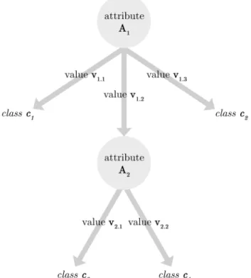
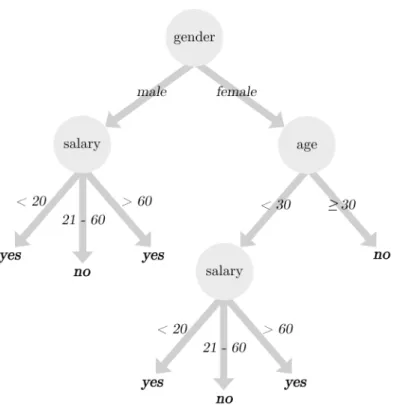
This thesis presents an alternative hyper-heuristic framework for constructing a different breed of data mining algorithms: decision tree building algorithms. Decision trees are tree-like graphs made up of nodes, branches and leaves where the nodes contain attribute names, the branches contain attribute values and the leaves contain target class values (see Figure 1.2). A decision tree can be used to classify objects by traversing it from the top down. At each step of the way, the branch taken is always the one whose value matches the value of the object’s attributes. The traversal process stops at one of the bottom leaves. The class specified by the leaf is the class assigned to the
Chapter 1 - Introduction
5
object. Decision trees are widely used in the data mining community as they are easy to read and understand as well as fast to traverse.
Figure 1.2: A Generic Decision Tree
A typical decision tree building algorithm builds a tree step by step by deciding, at each step, how to develop the next node in the tree using the training data set. The topmost node is the first to be created after which the rest of the tree is grown in a recursive manner. An example of such an algorithm is the popular ID3 (Quinlan, 1986). The vast majority of algorithms for building decision trees use this strategy. One of the procedures that usually varies from one algorithm to another is the heuristic used to choose which attribute should be placed at each node in the tree. ID3 uses a heuristic based on information gain to create nodes in a decision tree. The heuristic used to create tree nodes is crucial to the performance of the resulting decision tree, so much so that decision tree building algorithms are often
Chapter 1 - Introduction
6
defined, to some extent, by the heuristic they employ to create nodes (Buntine and Niblett, 1992; Liu and White, 1994).
One thing common to all decision tree building algorithms is that this heuristic is static throughout the whole tree building process. This brings us back to the problem mentioned earlier. There is no heuristic that is universally better at building decision trees. Different heuristics are suited for different data sets. Furthermore, there is no clear way of choosing which heuristic to use according to the data set at hand.
This work addresses this problem by proposing a hyper-heuristic decision tree induction algorithm. Our hyper-heuristic automatically chooses which heuristic to use according to the data set at hand. We do this by augmenting the standard decision tree building technique described earlier with a hyper-heuristic that, at each step of the way, is input with the current problem state and returns the heuristic to be used to handle that problem state. The problem state is the training data set while the output is the heuristic that chooses which attribute to use at the next tree node to be created. The hyper-heuristic manages this through a rule set: a number of if-then rules that map certain features of the data set to a heuristic (see Figure 1.3).
Figure 1.3: Hyper-heuristic for Decision Tree Induction
One can call this rule set the “brain” of the hyper-heuristic since it transforms our decision tree building algorithm into a hyper-heuristic capable of adapting the heuristic used for attribute selection according to the problem at hand.
Chapter 1 - Introduction
7
We present various ways in which such a rule set can be represented, mostly differing in the way the problem state is characterized (i.e. the data set features considered by the rule set). We explore two possible uses for each of these variants by defining two types of hyper-heuristics for decision tree building algorithms: specialized hyper-heuristics that are tailored for a data set from a particular problem domain and generalized hyper-heuristics that are expected to run reasonably well over a number of data sets from different problem domains. In all cases, we use a hyper-heuristic genetic algorithm for discovering a good set of rules.
All of these hyper-heuristics are tested on a number of real data sets picked from a wide variety of domains. We use data sets of different sizes with underlying classification models of varying complexity. The results obtained are compared to those achieved by a number of standard, non-adaptive decision tree building algorithms. We identify situations in which using such hyper-heuristics can yield decision trees of a higher predictive accuracy than the ones created by the standard methods. We also run experiments on synthetic data sets to try and understand how such hyper-heuristics are capable of adapting the heuristic used according to the problem state.
1.4 Contributions
This thesis offers contributions in the area of hyper-heuristics and data mining. The primary contribution of this thesis is the first set of approaches to develop decision-tree based data mining algorithms using hyper-heuristics. In fact, this represents one of the first few attempts at developing data mining algorithms in general using hyper-heuristics. A specific breakdown of the main contributions is as follows:
Chapter 1 - Introduction
8
1. A key factor for any hyper-heuristic is how to represent the problem state. We introduce, explore and evaluate five different ways how the problem state can be represented:
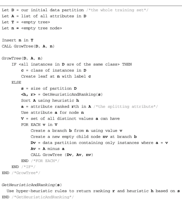
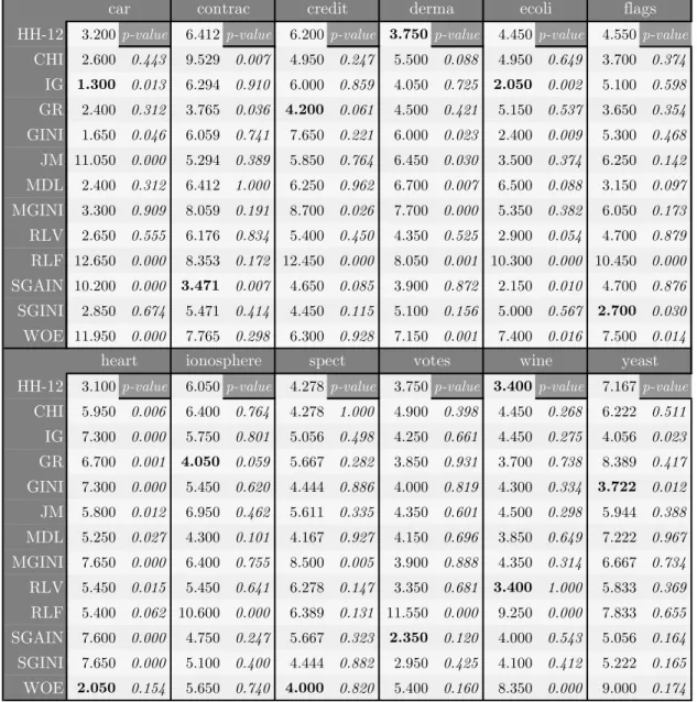
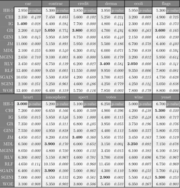
a. Using the number of instances in the partition to be split (sections 3.4 and 3.5).
b. Using the number of attributes left in the partition to be split (section 4.1).
c. Using the value count of the attributes left in the partition to be split (section 4.2).
d. Using the entropy of the attributes left in the partition to be split (section 4.3).
e. Using the maximum conditional entropy of the class attribute in the partition to be split (section 4.4).
2. Another key factor for any hyper-heuristic is the pool of low-level heuristics at its disposal. We explore and evaluate three different pools of heuristics for finding splitting attributes:
a. Using a single fixed heuristic for sorting the candidate splitting attributes while adapting the ranking of the chosen attribute (section 3.4).
b. Using a set of two heuristics for sorting the candidate splitting attributes as well as adapting the ranking of the chosen attribute (section 3.5).
c. Using a bigger set of five or twelve heuristics for sorting the candidate splitting attributes while always choosing the first-ranked attribute from the sorted list of attributes (sections 4.1, 4.2, 4,3 and 4.4).
3. We make a distinction between specialist hyper-heuristics (trained on a single data set from a particular domain) and generalist
hyper-Chapter 1 - Introduction
9
heurisitics (trained on a number of data sets from different domains) and we evaluate both approaches for each of the hyper-heuristics presented in this work.
4. In chapter 5 we present experimental evidence using synthetic data sets that tries to shed some light on when and why our hyper-heuristics work. These experiments suggest that the number of data sets used to train a hyper-heuristic for decision-tree building algorithms such as the ones presented in this work is related to the performance of the resultant decision trees (section 5.1). They also suggest that having a pool of training data sets with a variety of class distributions can help evolve more robust hyper-heuristics (section 5.2).
The PhD research described in this thesis has produced the following publication:
Vella A., Corne D. and Murphy C. (2009) Hyper-heuristic Decision Tree Induction. World Congress on Nature & Biologically Inspired Computing, 2009, pp. 409-414.
1.5 Thesis Overview
The rest of this thesis is structured as follows. Chapter 2 provides the necessary background to this thesis in the form of a literature review of hyper-heuristics and decision-tree building algorithms. In chapter 3 we discuss certain shortcomings of the current non-adaptive methods for building decision trees, thus explaining our motivation for using hyper-heuristics. We present the first version of our hyper-heuristic together with experimental results that compare it to standard methods on real data sets. Chapter 4
Chapter 1 - Introduction
10
presents four more variants of our hyper-heuristic. Each of these variants is again compared to standard methods on real data sets. In chapter 5 we try to understand how and when our hyper-heuristics perform well by running experiments on synthetic data sets. Chapter 6 lists our conclusions as well as possible future work.
Chapter 2 - Literature Review
11
Chapter 2
Literature Review
2.1 Hyper-heuristics
2.1.1 Origins and Early Approaches
The origin of the notion behind hyper-heuristics can be traced back to the 1960s (Fisher and Thompson, 1961; Crowston et al, 1963). This work investigated combinations of basic rules for job-shop scheduling. Using probabilistic learning they showed that combining these scheduling rules gave better results than applying any one of them separately. This notion was not revisited until 1985 (Smith, 1985) when Smith developed a hybrid genetic algorithm for solving the bin packing problem. This genetic algorithm used an indirect encoding approach in which a chromosome represented rules for producing the solution as opposed to the solution itself. In this work, a base heuristic was used to pack items of various sizes into bins while a genetic algorithm was employed to find the best ordering for these items. From 1985 until the late 1990s a series of works in the field of hyper-heuristics were carried out although the term “hyper-heuristic” was not introduced until 2000
Chapter 2 - Literature Review
12
(Cowling et al, 2000). What unites these works is that they all employ methods that conduct a search or operate in the space of heuristics (or parameters for heuristics) to solve a set of instances of a problem. This is in contrast to other search methods that work in the space of direct solutions. Syswerda (1991) and Fang et al (1993) both applied a genetic algorithm that used an indirect encoding to scheduling where a heuristic was used to fit an ordered list of tasks into a developing schedule. The genetic algorithm was used to find the optimal ordering for these tasks. Kelly and Davis (1991) applied a similar hybrid genetic algorithm approach to k-nearest neighbour to aid data classification while Ling (1992) used this technique for solving timetabling problems. Shing and Parker (1993) used a hybrid genetic algorithm to optimise parameters for a set of heuristics. Another notable study was that of Gratsch et al (1993; 1996),which used hill-climbing in a space of control strategies to find good algorithms for controlling satellite communication schedules.
Storer et al. (1992; 1995) identified the need to carry out a search in the heuristic space so as to generate a combination of problem-specific heuristics. They used a hill-climbing technique to search within this neighbourhood but they also suggested that other search techniques could be used such as genetic algorithms, tabu search or simulated annealing. The open-shop scheduling problem was revisited by Fang et al in 1994. This time they used a genetic algorithm to evolve a sequence of heuristics to be applied to the problem. In this work the authors comment on the advantages of using a genetic algorithm hybridized with a heuristic search where each chromosome represents an abstraction of a solution. Such hybridization avoids the need to represent a complete solution as an individual in the population of a genetic algorithm, thus facilitating the search performed by the genetic algorithm.
Chapter 2 - Literature Review
13
In Langdon (1995) a hybrid genetic algorithm was used to schedule the maintenance of electrical power transmission networks. This problem was revisited in Langdon (1996) in which genetic programming was used to evolve a schedule for the same purpose. Dorndorf and Pesch (1995) used evolutionary algorithms to evolve local decision rule sequences for production scheduling. Hybrid genetic algorithm approaches were used to solve a graph colouring problem in Fleurent and Ferland (1996), a bin-packing problem in Reeves (1996), a line-balancing problem in Schaffer and Eshelman (1996) and timetabling problems in Corne and Ogden (1997) and Terashima- Marín et al (1999). In Terashima-Marin et al (1999), an individual represented a series of instructions and parameters for guiding a search algorithm that builds a timetable. The instructions allowed the algorithm to switch its search strategy when a certain problem condition is met.
Zhang and Dietterich (1995; 1996) developed novel job-shop scheduling heuristics within a reinforcement learning framework while Minton (1996) presented a system that works by modifying elements of a template for a generic algorithm. This system was used to generate reusable heuristics for constraint satisfaction problems. Norenkov and Goodman (1997) proposed a system that conducts a search in the space of heuristics using evolutionary algorithms to solve multistage flow-shop scheduling problems. Hart and Ross (1998) evolved heuristic combinations for dynamic job-shop scheduling problems using a genetic algorithm. This concept was later applied by Hart et al (1998) to a real-world scheduling problem. The problem involved scheduling the collection and delivery of chickens from farms in different locations to multiple processing factories. This time two genetic algorithms were used, one to evolve heuristics for assigning orders and the other to evolve heuristics for scheduling the arrival of deliveries.
A novel search framework called “squeaky wheel optimization” was proposed by Joslin and Clements (1999) that works by iterating three stages named
Chapter 2 - Literature Review
14
construct, analyze and prioritize. In the construct stage, a heuristic is used to construct a complete solution using some priorities related to features of the problem being solved. In the analyze stage, the resultant solution is analyzed and “trouble spots” are identified. Trouble spots are elements in the solution that if improved are likely to increase the objective function score. In the prioritize stage the priorities are redefined according to the identified “trouble spots”. The idea is to operate the search in the space of priorities as opposed to the space of solutions. In the same year, Voudouris and Tsang (1999) proposed a hillclimbing algorithm that is re-run with a modified target function each time it gets stuck in a local minimum. The target function is changed through the use of problem-dependent features which carry costs and penalties.
2.1.2 Reinforcement Learning Hyper-heuristics
The literature contains several hyper-heuristics that use reinforcement learning. Such hyper-heuristics would typically utilize a pool of low-level heuristics and some technique for choosing which heuristic to apply to the solution at the different stages of the problem-solving process. The decision would be based on some sort of feedback relating to the heuristics’ past performance when applied to the problem. One such hyper-heuristic is the choice function hyper-heuristic which was first proposed by Cowling et al (2000). This hyper-heuristic iteratively modifies a candidate solution using a set of heuristics. The choice function chooses which heuristic to apply at each iteration by taking into consideration the past performance of each heuristic, the heuristic applied just before as well as the last time each heuristic has been called. This system was successfully applied to a hard scheduling problem in (Cowling et al, 2002a) and to a real-world nurse scheduling problem in (Kendall et al, 2002a). Further experiments in (Kendall et al, 2002b) confirmed that the choice function does adapt and choose intelligently which low-level heuristics to call in the order that best suits the search space and the problem being solved.
Chapter 2 - Literature Review
15
Narayek (2001) proposed a hillclimbing algorithm that has a set of heuristics at its disposal where each heuristic is assigned a weight value. At each iteration, the system always applies the heuristic with the largest weight value. The weight values are modified (adapted) according to the heuristics’ past performance during the search process. A similar heuristic-ranking system was presented by Burke et al (2003b) who applied this concept to a timetabling problem. This hyper-heuristic also made use of a tabu list that temporarily omits heuristics from being chosen if they do not improve the solution. Burke and Newall (2002) presented a hyper-heuristic framework for solving exam timetabling problems that iteratively adapts the ranking of exams left to schedule for a heuristic that inserts these exams into a developing timetable. A weighting system is again used to change the ranking of exams left to schedule as the algorithm progresses. A heuristic-ranking hyper-heuristic is described in (Pisinger and Ropke, 2007) for solving vehicle routing problems. This hyper-heuristic uses roulette wheel selection to choose which heuristic to apply at each iteration. The better the past performance of a heuristic, the higher its weight value and the higher the probability of it being chosen by the hyper-heuristic at the next iteration.
Dowsland et al (2007) proposed a novel hyper-heuristic embedded within a simulated annealing framework. The system was used to determine shipper sizes for storage and transportation – a complex problem with a massive search space. The hyper-heuristic employs a set of heuristics and the same heuristic-ranking technique is used where the heuristic with the highest weight is always chosen. A tabu list is also used for temporarily omitting heuristics that do not improve the solution. At each iteration, an acceptance mechanism is used to decide whether a new solution is accepted or not after the chosen heuristic is applied. The acceptance method for a move in the solution search space is based on simulated annealing but the temperature can go both up and down during the course of the hyper-heuristic run. A similar simulated annealing based hyper-heuristic was presented in the same year by Bai et al
Chapter 2 - Literature Review
16
(Bai et al, 2007a). This time, the hyper-heuristic employs a short-term memory so that only the recent performance of the heuristic is reflected in its weight value. The authors’ reason for using such a technique is that the search for a good solution proceeds in a dynamic environment as the region of the search space being explored changes and the information gathered during the initial stages may not be useful later in the search. The exam timetabling problem was revisited by Burke et al (2008b). This work presented a hyper-heuristic that combined reinforcement learning (through hyper-heuristic-ranking) with the Great Deluge acceptance mechanism (Kendall and Mohamad, 2004a).
2.1.3 Tabu-Search Hyper-heuristics
Burke et al (2003b) proposed a tabu-search hyper-heuristic for solving timetabling problems. The system builds a timetable iteratively by applying a heuristic from a set at each iteration. The heuristic to be applied is chosen on the strength of its past performance. If, once applied, the heuristic does not improve the solution, it is inserted in a tabu list for some time so as to temporarily prevent it from being chosen. This approach was later integrated within a simulated annealing framework by Dowsland et al in 2007 for the purpose of searching for good combinations of low-level heuristics to determine shipper sizes in transportation problems. The timetabling problem was also tackled by Kendall and Hussin (2005) who used a hyper-heuristic to build timetables in the same iterative manner as described in Burke et al (2003). In this work, all heuristics are tried out on the solution at each iteration but only the heuristic that yields the best improvement is actually applied to the solution before moving on to the next iteration. After the best heuristic is applied to the solution, it is inserted in a tabu list so as to exclude it from being chosen by the hyper-heuristic for some time. The authors argue that such a system allows for a balance between intensification (best heuristic is always chosen) and diversification (heuristic is excluded for some time after it is applied) in terms of the search process.
Chapter 2 - Literature Review
17
In Cowling and Chakhlevitch (2003) and Chakhlevitch and Cowling (2005), the performances of various hyper-heuristics that make use of a collection of low-level heuristics were investigated by testing them on personnel scheduling problems. Four hyper-heuristics that use some kind of tabu list were compared to various other hyper-heuristics including four Peckish hyper-heuristics (Corne and Ross, 1995). The Peckish algorithm works by always applying the heuristic that gives the biggest improvement in terms of the solution objective function. If none of the heuristics manage to improve the solution, a random one is chosen and applied. The results of their experiments suggested that using smaller sets of low-level heuristics was not so effective and that the performance of a hyper-heuristic is determined to a great extent by the quality of the low-level heuristics used. The same conclusion was arrived at by Özcan et al (2008) who compared the performance of genetic algorithms and memetic algorithms to a number of hyper-heuristic methods that use various combinations of different heuristic selection and acceptance methods.
In Burke et al (2005a; 2007a) and Qu and Burke (2008), tabu search based hyper-heuristic methods were used to find heuristic lists to solve timetabling problems. The search space of the tabu search consisted of all possible permutations of low-level graph colouring heuristics that construct timetables. In Burke et al (2007a), the authors highlight one advantage of conducting a search in the heuristic space by saying that moving in the heuristic space can result in jumps within the solution space that might not be always possible if the search is conducted in the solution space. They do however mention that a search in the heuristic space might make some solutions unreachable. The authors also conclude that the larger the number of low-level heuristics available to the hyper-heuristic, the better it may perform provided a reasonable search time is given.
Chapter 2 - Literature Review
18
2.1.4 Hyper-heuristics that use Problem State Representation
In Petrovic and Qu (2002) and Burke et al (2002), a system was proposed that matches the features of some instance of a timetabling problem with case problems stored in a case base. Each entry in the case base would contain the heuristic most suited for solving the case problem. Ross et al. (2002) successfully used a Michigan-style (Freitas, 2002) learning classifier system called XCS (Wilson, 1995) to evolve a set of rules that dictate which heuristic to use when some particular problem state is encountered while solving a bin-packing problem. The problem state is represented by the number and size of items left to pack. This way, the hyper-heuristic manages which heuristics are used as well as when they are used throughout the problem-solving process. Marín-Blázquez and Schulenburg (2006; 2007) extended this system by introducing a multi-step reward system. The produced algorithms generalized well on both training and unseen data. The authors stressed the importance of the choice of representation for the problem state in the hyper-heuristic rules. In Ross et al (2003), a messy genetic algorithm was used to evolve the same kind of hyper-heuristic rules described in Ross et al (2002). As in their previous work, each chromosome represents a set of rules that match heuristics to problem states. In the first generation of the genetic algorithm, each chromosome was applied to 5 bin-packing problems chosen randomly from a set of training problems. In the subsequent generations, each chromosome was assigned one random problem so as to calculate its fitness. The fitness value was taken to be the difference between the results obtained by the hyper-heuristic and the best result obtained by any single hyper-heuristic on the same problem. The same concept was successfully applied to timetabling problems using graph colouring heuristics in (Ross et al, 2004; Ross and Marín-Blázquez, 2005), 2D cutting stock problems in (Terashima-Marín et al, 2006) and constraint satisfaction problems in (Terashima-Marín et al, 2008). The 2D strip packing problem was tackled in a similar manner by Garrido and Riff (2007a; 2007b) but their heuristic was online so the evolved
hyper-Chapter 2 - Literature Review
19
heuristic rules could only be used to solve the same problem instance that was used for training.
Thabtah and Cowling (2008) suggested mining hyper-heuristic rules from the solution run of Peckish (Cowling and Chakhlevitch, 2003) – a robust but slow hyper-heuristic. The data set to be mined would contain all the improving moves of Peckish. For each improving move, the data set would contain the heuristic applied as well as the features of the problem state before the heuristic was applied. Data mining could then yield hyper-heuristic rules that would dictate which heuristic to use according to the features of the current problem state. The authors suggest that such rules could replace the slower Peckish hyper-heuristic. Burke et al (2008c) also proposed using data mining to speed up a hyper-heuristic. This time, data mining is used to skip the step of calculating the objective function value of the candidate solution at each iteration. To achieve this, the authors proposed a system that, after training, can recognize patterns hidden in good candidate solutions, which can then be used to classify newly obtained solutions without calculating their fitness value.
2.1.5 Genetic Programming Hyper-Heuristics
Genetic programming was used to evolve priority dispatching rules for machine scheduling problems in (Dimopoulos and Zalzala, 2001; Ho and Tay, 2005; Geiger et al, 2006). Geiger et al (2006) presented a genetic programming system called SCRUPLES (Scheduling Rule Discovery and Parallel Learning System) to carry out a number of experiments with training sets containing problem instances of various sizes. It was observed that the generalizing ability of the learned rules improved as the number of training instances approached 10 but then worsened after 10. Tay and Ho (2008) extended their earlier work so as to evolve dispatching rules for multi-objective job-shop problems.
Chapter 2 - Literature Review
20
Genetic programming has also been used to construct heuristics for the minimisation of binary decision diagrams (Schmiedle et al, 2002), to aid compiler optimization (Stephenson et al, 2003), to solve the travelling salesman problem (Oltean and Dumitrescu, 2004; Keller and Poli 2007a; 2007b), parallel machine scheduling problems (Jakobovic et al, 2007) and a biobjective knapsack problem (Kumar et al, 2008). Fukunaga (2002) proposed a system called CLASS to evolve algorithms for solving satisfiability testing problems. CLASS maintains a population of such algorithms over several cycles and uses a composition operator to create new algorithms at the end of each cycle. The performance of CLASS was improved in (Fukunaga, 2004) by limiting the size of the trees representing the candidate algorithms. Heuristics for the same kind of problems were evolved by Bader-El-Din and Poli (2007) using a grammar-based genetic programming system.
Tavares et al (2004) used genetic programming to evolve evolutionary algorithms that solve a function optimization problem. The hyper-heuristic works by evolving an effective mapping function that maps a genotype to a phenotype. Oltean (2005) also presented a hyper-heuristic that produces evolutionary algorithms using genetic programming. The system works by treating an array of data as a population where each array member is called a register. Genetic programming is used to evolve instructions that operate on these registers in the same way genetic operators work on a population. The system was successfully applied to function optimisation, a travelling salesman problem and a quadratic assignment problem.
Burke et al (2006a) used tree-based genetic programming to automate the construction of heuristics for online bin packing problems. It was noted that in most of the runs, the genetic program managed to evolve some kind of variant of the well-known, human-designed First-Fit algorithm (Johnson et al, 1974). This work was followed by Poli et al (2007) who used a linear genetic programming system to construct heuristics for offline bin packing problems.
Chapter 2 - Literature Review
21
In (Burke et al, 2008d), genetic programming was used to evolve disposable heuristics that work out the score for each possible allocation in a 2D strip packing problem so that the allocation with the highest score is chosen at each step of the algorithm.
2.1.6 Hyper-Heuristics for Machine Learning
In Abe and Yamaguchi (2004) an inductive learning system called CAMLET (Suyama et al, 1998) is used for meta-learning. In this work, CAMLET constructs classification algorithms from a repository of methods according to a given data set. The repository of methods consists of various building block components from a selection of inductive learning methods. A control structure is then used to describe the relationship between these building blocks. Delibasic et al (2011) proposed a platform for storing reusable decision tree algorithm components such as attribute selection, split evaluation, stopping criteria and pruning strategies. A component-based framework called WhiBo is then used to recombine these components into complete decision tree building algorithms.
Pappa and Freitas (2006) used grammar-based genetic programming to evolve rule induction algorithms, having presented the original idea in Pappa and Freitas (2004). A broad category of rule induction algorithms operate via sequential covering: an initial rule is generated, covering some of the dataset, and additional rules are generated in order until the entire dataset is covered. There are several alternative ways to generate the initial and subsequent rules. For instance, we may either start with a very general high-coverage (but low accuracy) rule, and add conditions until accuracy and/or coverage move beyond a threshold. Or, we may start with a very precise rule and gradually remove conditions. In Pappa and Freitas (2006), the encoding covered a vast space of possible ways to organize this process. Pappa and Freitas (2007)
Chapter 2 - Literature Review
22
shows how the same concept can be applied for multi-objective genetic programming.
Barros et al. (2011) recently proposed the idea of using genetic programming to evolve decision tree induction algorithms but no implementation has been reported yet.
2.1.7 Other Hyper-heuristics
Cowling et al (2002b) proposed using a genetic algorithm as a heuristic-selector for a scheduling problem. Each individual represents a sequence of heuristics and the heuristics encoded by the best individual of each generation are applied to the solution. Ahmadi et al (2003) used a variable neighbourhood search algorithm to find sequences of parameterized constructive heuristics to solve examination timetabling problems. A variant of the same algorithm was presented in Qu and Burke (2005). In this work, the authors highlighted the difference between working in the heuristic search space and solution search space. Two heuristic lists that have very little differences between them can result in two very different timetables. So the same effort within the high level searching is capable of exploring a much larger part of the solution space than a similar amount of effort used by local search based methods applied directly to solutions.
Ayob et al (2003) presented a novel heuristic acceptance criteria called the Exponential Monte Carlo with Counter method for hyper-heuristics that work by iteratively modifying a complete solution using a pool of low-level heuristics. This method works by always accepting solutions that improve on the previous one while the probability of accepting non-improving solutions decreases as time passes but increases as the number of non-improvement iterations increases. Another novel heuristic acceptance criterion called the Great Deluge was proposed by Kendall and Mohammad (2004a). This
Chapter 2 - Literature Review
23
mechanism only accepts improved solutions and tends to favour diverse solutions as more iterations of the program are carried out. This technique was used in a hyper-heuristic to solve the channel assignment problem for cellular communication. Burke and Bykov (2008) proposed a memory-based heuristic acceptance mechanism that accepts a new solution by comparing its objective function value with that of L solutions ago. The motivation behind this technique is to allow for some worsening moves thus helping to avoid local minima, while still making “intelligent” use of information collected during search.
Asmuni et al (2005) used a fuzzy hyper-heuristic system to solve course timetabling problems. The system uses fuzzy weights to decide which event to schedule while constructing the timetable. A variant of exhaustive search is used to discover a good shape for the fuzzy membership functions. Bai and Kendall (2005) proposed a hyper-heuristic based on simulated annealing to solve a space allocation problem. This hyper-heuristic was later applied by Bai et al (2006) for timetabling problems. Burke et al (2005b) presented the ant colony algorithm (Dorigo et al, 1991) as a hyper-heuristic to solve a real world scheduling problem. The same algorithm was later used by Chen et al (2007) to solve a sport timetabling problem. Burke et al (2006b) presented a case-based system for heuristic selection to solve timetabling problems.
In Vázquez-Rodríguez et al (2007a), a genetic algorithm was used to solve the first stage of a scheduling problem after which a hyper-heuristic was used to continue working on the problem for the second stage. The hyper-heuristic itself consisted of a combination of various dispatching rules evolved through the use of a genetic algorithm. Bhanu and Gopalan (2008) presented a hyper-heuristic that works on top of three meta-hyper-heuristics to solve a grid resource scheduling problem. The hyper-heuristic works above the meta-heuristics and the meta-heuristics work on candidate schedules. The three meta-heuristics are a genetic algorithm combined with local search, a genetic algorithm with a
Chapter 2 - Literature Review
24
mutation operator inspired by simulated annealing and a genetic algorithm that uses a tabu list.
2.2 Decision Trees
2.2.1 Decision Trees for Classification
A decision tree is a tree structure that can be used to classify data instances into some target class (Freitas, 2002). The tree structure is made up of attribute names at the nodes, attribute values at the branches and target classes at the leaves (see Figure 1.2). When a new instance needs to be classified, the values of its attributes are tested against the attributes found in the nodes of the tree, starting from the single topmost node and going down to the bottom. The branch taken is the one whose attribute value matches the one in the instance. The tree is traversed in this way until a leaf is met – the class at the leaf would be the class assigned to that instance.
Decision trees have been successfully used in virtually any field that involves some form of data mining. Using decision trees for data mining comes with many advantages: a decision tree is very easy to read and understand by humans as long as the tree is not too large, the most important attributes for classification can be easily identified as the ones towards the top of the tree, most decision tree building algorithms are non-parametric and they do not require an expert in domain of the data that is being mined.
2.2.2 Algorithms for Building Classification Trees
The majority of decision tree-building algorithms build decision trees in a recursive manner, using a greedy, divide-and-conquer method, by adding one attribute at a time to a growing tree. Such an algorithm works in a top-down
Chapter 2 - Literature Review
25
fashion, starting with the full training data, partitioning it into smaller subsets by choosing a splitting attribute, and then recursing this partitioning process on each of the subsets. This procedure stops when all the instances in the partition belong to the same class or when the partition satisfies some stopping condition.
Stopping conditions are used to produce trees that are not overly complex and that do not overfit the training data. Overfitting happens when the classifier captures noisy data and/or spurious relationships (Freitas, 2002). Noisy data refers to errors in the training data whilst spurious relationships are relationships between attributes in the training data that are not statistically significant enough to help us in classifying future unseen data instances. Another effective way of dealing with this problem is by using a pruning technique. This involves growing a full-sized tree that perfectly fits the training data after which the pruning algorithm is used to reduce the size of the tree by removing certain nodes and branches that are believed to be insignificant to the predictive accuracy of the whole decision tree.
Morgan and Sondquist (1963) presented one of the earliest works on decision tree building algorithms. They proposed a system called AID (Automatic Interaction Detection) that finds binary splits on ordinal and nominal attributes that most reduce the sum of squares of an interval target from its mean. Lookahead split searches were allowed whereas cases with missing values were excluded. The algorithm stopped splitting the data when the reduction in sum of squares is less than some constant multiplied by the overall sum of squares. Other similar decision tree induction programs followed such as MAID (Gillo, 1972), THAID (Morgan and Messenger, 1973) and CHAID (Kass, 1980). CHAID (CHi-squared Automatic Interaction Detector) is a decision tree induction algorithm that finds non-binary splits based on adjusted significance testing. When building a tree, splitting attributes are
Chapter 2 - Literature Review
26
chosen using the chi-square criterion. Splitting stops when the smallest adjusted p-value is greater than some user-defined threshold.
Breiman et al (1984) proposed the well-known CART. This decision tree building algorithm uses the Gini index for finding binary splits that yield the “purest” partitions with respect to the classes. Breiman et al noted that the Gini index can yield splits that are unbalanced with respect to size if the number of classes is large. In such cases, it was suggested that the twoing rule should be used instead of the Gini index. CART does not use stopping rules when building trees, instead it prunes fully grown trees using a technique called cost complexity pruning that requires the use of a pruning data set separate from the training set used for growing the decision tree. CART can also build trees with nodes made up of linear combinations of attributes. These combinations are found using a hill climbing method which slows down the building process of the decision tree. Other disadvantages of having such combinations of attributes in the decision tree nodes is that such nodes would be harder to interpret and they ultimately do not guarantee a more accurate decision tree. This method for finding multivariate splits was later extended by Murthy et al (1993) to include randomization for escaping local minima. ID3 is another well-known algorithm that uses top-down induction for building decision trees. This was first proposed by Quinlan in 1979 but the last and definitive version was presented in (Quinlan, 1986). Quinlan argued that since there exist multiple trees that can classify all the objects in the training set as accurately as possible, the theory of Occam’s Razor dictates that one should go for the simplest tree as it is more likely to capture some meaningful relationship between an object’s class and the values of its attributes. For this reason, a simple tree would be expected to have a higher probability of classifying correctly objects outside the training set than a more complex one. This argument was later refuted by Domingos (1998) who presented various theoretical arguments supported by empirical evidence that though simplicity
Chapter 2 - Literature Review
27
itself might be a desirable attribute, it does not guarantee greater accuracy. Nevertheless, Quinlan first suggested using the information gain criterion as an attribute selection measure as it will always tend to yield very simple trees. Various strategies for dealing with missing values in both the training set and test set were discussed. The chi-square measure was suggested as a stopping criterion when building trees. Quinlan (1987) later suggested using reduced error pruning instead of stopping for producing trees with better accuracy. Quinlan also recognized that the information gain measure can unjustly favour attributes with many values. For this reason he recommended using the gain ratio criterion instead. ASSISTANT (Cestnik et al, 1987) overcame this problem by restricting the tree to binary splits only. Cestnik et al argued that the process of merging different attribute values for binary splitting helped the information gain criterion overcome the problem of favouring attributes with many values. Norton (1989) presented the IDX algorithm. This is like the ID3 algorithm with the added capability of performing lookahead when building trees so that it uses information gain to choose combinations of nodes on different levels of the tree as opposed to just one node at a time. Pal et al (1997) proposed using a genetic algorithm to fine-tune the nodes of a decision tree after it is built by an ID3-style algorithm. Their method, called RID3, was presented as an alternative to ID3 for problems that work on real data. Esmeir and Markovitch (2006) presented an alternative to RID3 called LSID3. The proposed learner uses a lookahead technique that tries to estimate the size of the smallest possible tree after splitting with each attribute. The attribute chosen to split the data is the one that yields the smallest tree.
Quinlan extended his ID3 algorithm to create one of the most widely-used classifiers: C4.5 (Quinlan, 1993). This program builds trees using the gain ratio criterion. It can also handle continuous attributes by choosing a threshold so as to split the attribute into two discrete sets: one containing values above the threshold and another containing values below or equal to the threshold. C4.5
Chapter 2 - Literature Review
28
can also be configured to consider attribute costs when building a tree. A post-pruning technique called error-based post-pruning is preferred to stopping as it is argued that this produces more reliable trees. This pruning technique does not make use of a separate pruning set, instead it prunes trees by replacing nodes with leaves if it improves the upper confidence limit of the predicted error rate. The C4.5 algorithm was later revised and extended in Quinlan (1998), the result of which was the commercial C5.0 algorithm. Amongst many other things, C5.0 improved the speed at which the decision trees are built, the memory usage as well as the size of the resultant decision trees.
Loh and Shih (1997) presented QUEST (Quick, Unbiased, Efficient, Statistical Tree), a binary-split decision tree algorithm that extends an earlier algorithm called FACT (Loh and Vanichsetakul, 1988). QUEST uses an unbiased attribute selection method in terms of number of values per attribute. For creating a node, it uses the F-statistic to first choose which attribute to split on. This is done before any of the attributes are actually split, giving QUEST an edge in terms of CPU time when compared to algorithms like CART that try to split each and every attribute before choosing one. QUEST then performs linear discriminant analysis for choosing split points, also allowing linear combinatons of attributes in a node. Kim and Loh (2001) extended this work to produce CRUISE (Classification Rule with Unbia