BARRODALE COMPUTING SERVICES LTD. BCS Grid Extension for PostgreSQL (Linux Version) Programmer s Guide

(1)

BARRODALE COMPUTING SERVICES LTD.

BCS Grid Extension for PostgreSQL

(Linux Version)

Programmer’s

Guide

(2)

(3)

BCS Grid Extension for PostgreSQL

(Linux Version) Programmer’s Guide

 Barrodale Computing Services Ltd.

(4)

(5)

P R O G R A M M E R ’ S G U I D E

List of Figures

Figure 1: A 3D depth-easting-northing grid with temperature/salinity/pressure data. ... 2

Figure 2: A 2D grid with two spatial domains. ... 6

Figure 3: A 2D grid with different domains (space and time). ... 7

Figure 4: Parts of a grid. ... 8

Figure 5: A 2D grid showing grid coordinates (sample positions). ... 9

Figure 6: A 3D grid showing real-world coordinates and nonuniformly-spaced points. ... 10

Figure 7: The 3x4 grid, shown in grid coordinates. ... 11

Figure 8: The grid after the application of nonuniform spacing on the vertical axis. ... 12

Figure 9: The grid after rotation and scaling. ... 13

Figure 10: Two views of the same grid – in grid coordinates and in real-world coordinates. ... 14

Figure 11: An orthogonal extraction... 17

Figure 12: A radial extraction. ... 18

Figure 13: An oblique extraction. ... 19

Figure 14: Interpolation between grid points. ... 20

Figure 15: N-linear interpolation. ... 21

Figure 16: Updating temperature t 211 to t´211. All other values remain unchanged. ... 23

Figure 17: Extending a grid by 1 time period. ... 23

Figure 18: Replacing a portion of a grid. ... 24

Figure 19: Combining {X,Y} grids for 5 different times into a single {X,Y,time} grid. ... 25

Figure 20: Merging XY grids for different time periods to form a single, longer grid. ... 26

Figure 21: Unioning a salinity depth-time grid and a temperature depth-time grid to form a grid with both salinity and temperature. ... 27

Figure 22: Original 2D 2x2 grid. ... 36

Figure 23: Final 1D grid with 11 grid points. ... 37

Figure 24: A Radial and a Radial Set. ... 130

Figure 25: GRDRadialSetExtract example. ... 133

Figure 26: Example of a rectilinear grid (grey) generated from a radial set (red) using the GRDFromRadial function. ... 136

Figure 27: Fusing three grids. ... 137

Figure 28: Fusing does not interpolate between grids. ... 139

Figure 29: Disallowed GRDValueUpdate example. ... 155

Figure 30: "Rotated Grid" Transformation: with translation but no rotation. ... 239

Figure 31: "Rotated Grid" Transformation: with both rotation and translation. ... 240

Figure 32: Cone at time 300. ... 255

Figure 33: Cone at time 310. ... 256

Figure 34: Horizontal slice of cone. ... 262

Figure 35: Vertical slice of cone. ... 264

Figure 36: Grid Import Client main screen. ... 271

Figure 37: Grid Import Client main screen with connection information filled in. ... 272

Figure 38: Source Files filled in. ... 273

Figure 39: Primary IDV Window. ... 276

Figure 40: IDV "Dashboard". ... 277

Figure 41: IDV Plugin Manager. ... 278

Figure 42: Selecting BCS Grid as the New Data Source. ... 279

Figure 43: BCS Grid Source Data Chooser. ... 280

Figure 44: Unsuccessful Connection Attempt error message. ... 280

Figure 45: List of tables filled in. ... 281

Figure 46: Grid selected, and subsetting buttons enabled... 282

Figure 47: Times Panel with “Seconds Since 1970” representation. ... 283

(14)

Figure 49: Data Selector window with Data Source, Variable, Visualization Method, and Times

values selected. ... 285 Figure 50: Visualization of extracted data. ... 286

(15)

Documentation Conventions

This section defines the conventions used in this document. The conventions include typographical conventions and icon conventions.

Typographical Conventions

This manual uses the following typographical conventions:

Convention Meaning

KEYWORD Programming language keywords (i.e., SQL, C

keywords) appear in a serif font. italics

italics

italics

New terms, emphasized words, and variable values appear in italics.

User input Computer generated text (e.g., error messages) and user input appear in a non-proportional font.

<POSTGRESQLDIR> _{The directory where the PostgreSQL server is}

installed. The name varies according to the operating system (flavor of Linux) and the version of

PostgreSQL. For example, under Ubuntu and PostgreSQL 8.4 the directory is

/usr/lib/postgresql/8.4

)ehportsopa( ۥ An apostrophe is used in the plural form of data types

(16)

Icon Conventions

This manual uses the following icon conventions to highlight passages in the manual:

Icon Label Description

Warning: Identifies paragraphs that contain vital

instructions, cautions, or critical information.

Important: Identifies paragraphs that contain significant information about the feature or operation that is being described.

Tip: Identifies paragraphs that offer additional

details or shortcuts for the functionality that is being described.

(17)

What’s New in This Version?

The following table lists the features that have been added to this version of the BCS Grid Extension:

Feature Manual Sections Where Feature is Described.

(18)

(19)

Chapter 1: Gridded Data

and the BCS Grid

Extension – An

Introduction

This chapter defines what is meant by “gridded data” and discusses a number

of areas of science that are concerned with gridded data. It then introduces some terminology that is useful when talking about gridded data, discusses the role of databases in storing gridded data, and introduces the BCS Grid

Extension as a tool for managing gridded data.

What Is Gridded Data?

Gridded Data is data that is organized as a multi-dimensional rectangular array of grid points containing values. Gridded data occurs in many specialized application areas such as meteorology, oceanography, remote sensing, hydrology, surveying, civil engineering, astronomy, non-destructive testing, medical imaging, social sciences, and exploration systems for oil, natural gas, coal, and diamonds. These datasets range from simple, uniformly-spaced grid points along a single dimension to multi-dimensional grids containing several different types of grid values.

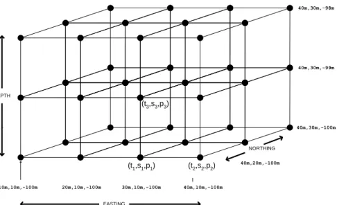
As an example, consider a dataset created by recording ocean measurements (temperature, salinity, and pressure) every hour at spacings every one meter in depth and every ten meters in two horizontal dimensions (northing and easting, or latitude and longitude). This dataset is a 4-dimensional (4D) grid having three spatial dimensions (northing, easting, and depth) and one temporal dimension. Three variables (temperature, salinity, and pressure) are attached to each grid point, as illustrated in the following diagram, which shows a portion of just three of the dimensions (depth, easting, and northing). Three of the

Chapter

(20)

points on the grid, picked arbitrarily, have been labeled with temperature, salinity and pressure values (ti,si,pi).

10m,10m,-100m 40m,30m,-100m 40m,20m,-100m 40m,10m,-100m 30m,10m,-100m 20m,10m,-100m 40m,30m,-99m 40m,30m,-98m (t₁,s₁,p₁) (t₃,s₃,p₃) (t₂,s₂,p₂) EASTING NORTHING ` DEPTH

Figure 1: A 3D depth-easting-northing grid with temperature/salinity/pressure data.

Application Areas for Gridded Data

Grids in Modeling Applications

Broadly speaking, gridded data arises in two main areas of application:

modeling applications (often involving the numerical solution of differential equations as difference equations) and data analysis applications (which are discussed in the next section). Examples of modeling applications in which grids play an essential role are as follows:

Meteorology: Grids of meteorological data are central to the prediction of weather on both local and global scales. While satellite and other forms of imagery provide information on the current weather, these images are snapshots of the present and past, whereas grids provide the predictive power needed for weather-related decisions about the days ahead. Typically, 3D grids are populated with estimated values of physical parameters such as temperature, pressure, wind speed, and relative humidity, and the evolution of these values over time is predicted by solving sets of difference equations. The result is a 4D space-time grid of predicted values of the physical parameters. Such grids, generated over various scales, are often sub-sampled and interpolated and the results are then projected for display and interpretation. Many weather-related data products may also be generated from the information in these grids. Major producers of meteorological grids are civilian and military weather forecasting

(21)

(https://www.fnoc.navy.mil/) in the USA, and the MET Office in the UK

(http://www.met-office.gov.uk/).

Oceanography: Grids are used in modeling ocean circulation and ocean-atmosphere interaction. These applications are similar to meteorological applications but also take the shorelines and subsurface ocean physical parameters into account in the modeling, and typically have longer time horizons than for weather prediction.

Climatic modeling: Global climate modeling is often based on solving difference equations for grids encompassing the Earth’s surface. In this case, the time horizons are often decades or centuries. (See

http://www.arsc.edu/challenges/pdf/fall2000.pdf.)

Fluid dynamics: Certain other types of mathematical modeling are carried out on grids, and fluid dynamics is just one example. The motion of a fluid in response to a forcing function can be modeled using finite element analysis applied to a 3D grid.

Other specific examples of modeling applications involving grids are hurricane analysis, optimal extraction of mine resources and petroleum reservoirs, air quality control strategies, and forest fire burn area predictions.

Grids in Data Analysis

Nondestructive Testing: Grids of 3D data are increasingly used in the nondestructive testing of materials using ultrasonic inspection techniques. These are particularly vital to the aviation industry for inspection of aircraft components to detect defects and delaminations. In these applications, a transducer is moved over the surface in a raster pattern and an ultrasonic

pressure trace is recorded at each position. Hence, the three dimensions are x, y, and t (which is related to depth). These datasets may be processed in various ways to enhance their resolution, and features of interest may be analyzed using special-purpose visualization tools (http://www.barrodale.com/nde/index.htm). Also, gridded data collected during one inspection may be compared with data obtained for the same component during an earlier inspection, to detect any significant changes.

Geophysics: Prospecting for natural resources such as oil and gas involves the acquisition, analysis and interpretation of gravimetric, electromagnetic and seismic data stored as large 2D, 3D and, sometimes, 4D grids. Here, the data collected is extensively processed both before and after grid formation. These grids are collected over large areas, both on land and over the ocean floor. A common application is to generate 2D slices along an arbitrary vertical plane (cross-sections) through this data. It is also possible to combine several time-separated datasets and to model the changes within the volume (e.g., resulting

(22)

from petroleum removal). In addition to oil and gas prospecting, other areas of geophysics that involve grids include mineral prospecting (e.g., diamonds), geothermal analysis, and plate tectonics modeling.

Medical Imaging: Various medical imaging techniques have recently come into existence that can produce 3D (and occasionally 4D) gridded data. These include ultrasonic pulse echography, computed axial tomography (CAT), magnetic resonance imaging (MRI), and positron emission tomography (PET).

See http://www.barrodale.com/grid_Demo/index.html (the first demo provided)

for a demonstration of retrieving oblique 2D slices from 3D datasets. This demo utilizes a 1.6GB 3D grid from a Visible Human Project file system containing 1871 parallel raster images spaced at 1mm intervals of a cryosectioned male subject.

Satellite Imaging (Remote Sensing): It is often desirable to store satellite image data in its raw unprojected swath form so that it may later be extracted in a variety of user-specified projections. The alternative – storing the image as a raster in an arbitrarily chosen projection – introduces two problems:

1) The reprojected data must be stored at a higher resolution to reduce information loss due to resampling artifacts like aliasing.

2) Some calculations done on observed datasets are very sensitive to the effects of resampling (for example, edge detection), regardless of the resolution of sampling.

For these reasons, the BCS Grid Extension has a special feature that allows the input and storage of unprojected satellite swath data as a grid, and provides mechanisms for the data to then be extracted in a user-specified projection. Other specific examples of data analysis applications based heavily on grids are aerial site mapping, linear corridor identification, watershed delineation,

hydrographic surveying, highway engineering, and demographic predictions.

Grid Concepts

In this section we will present some of the concepts used to describe grids and the operations performed on grids.

The Dimensions of a Grid

Gridded data can come in a variety of shapes and sizes. By shape, we mean the number of dimensions the grid has and by size, we mean the number of points

(23)

in each dimension. The BCS Grid Extension supports grids of 1, 2, 3, and 4 dimensions1_{. Examples include:}

1D grid: a set of temperature measurements taken at various depths

along a vertical line extending from the sea surface to the ocean bottom (a grid with a depth dimension).

2D grid: the combination of several of these 1D grids taken along a

straight east-west line (a grid with a depth dimension and an easting dimension).

3D grid: the combination of several of these 2D grids taken along a

straight north-south line (a grid with a depth dimension, an easting dimension, and a northing dimension).

4D grid: the combination of several of these 3D grids, each captured at a specific time (a grid with a depth dimension, an easting

dimension, a northing dimension, and a time dimension).

Figure 1 illustrates a 3D grid (the dimensions being easting, northing, and depth), while Figure 2 illustrates a 2D easting-depth grid. In each figure, three of the points on the grid, picked arbitrarily, have been labeled with temperature, salinity and pressure values (ti,si,pi).

1

Technically, it supports just grids with four dimensions, but lower dimension grids can be represented by setting the number of points for one or more dimensions to one.

(24)

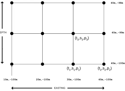
10m,-100m 40m,-100m 40m,-100m 30m,-100m 20m,-100m 40m,-99m 40m,-98m (t₁,s₁,p₁) (t₃,s₃,p₃) (t₂,s₂,p₂) EASTING ` DEPTH

Figure 2: A 2D grid with two spatial domains.

Each grid dimension can have a different number of sample positions. In Figure 2, for instance, the Easting dimension has four sample positions while the Depth dimension has three sample positions.

The individual dimensions of an array may or may not have the same domains. The grids illustrated in Figure 1 and Figure 2 are both based on spatial domains (measured in meters). Figure 3 below illustrates a grid with one spatial domain (depth) and one temporal domain (time, measured in seconds).

(25)

P R O G R A M M E R ’ S G U I D E 5sec,-100m 25sec,-100m 20sec,-100m 15sec,-100m 10sec,-100m 25sec,-99m 25sec,-98m (t₁,s₁,p₁) (t₃,s₃,p₃) (t₂,s₂,p₂) TIME ` DEPTH 25sec,-100m

Figure 3: A 2D grid with different domains (space and time).

Parts of a Grid – Some Terminology

The terms grid point, dimension, sample position, and variable have already been introduced: a grid is a set of grid points, organized along dimensions, storing data called variables. The dimensional axes can be considered variables, specifically referred to as coordinate variables. Each of the

coordinates of a grid point corresponds to a sample position – a position along one of the dimensional axes. The ordered list of sample positions of a grid point are called its grid coordinates. Metadata about the grid is stored in attributes. Attributes may be global(referring to the entire grid) or they may refer to specific variables. The following figure illustrates these concepts.

(26)

5sec,-100m 25sec,-100m 20sec,-100m 15sec,-100m 10sec,-100m 25sec,-99m 25sec,-98m (t₁,s₁,p₁) (t₃,s₃,p₃) (t₂,s₂,p₂) TIME ` DEPTH 25sec,-100m

Depth Profiles at Latitude 49o_{N, Longitude 128}o_W _{Global attribute}

Dimension (a Coordinate Variable)

Sample Positions Mesh Lines

Variables

Attribute (name of dimension)

Variable t may have attributes such as Name (“temperature”)

and Units (degrees Celsius)

Grid Points

Figure 4: Parts of a grid.

Note that the “Mesh Lines” shown above do not actually form part of a grid; they are shown just to illustrate the alignment of grid points.

Grid Spacing

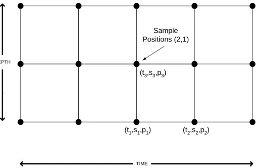
There are two ways to describe the position of a grid. One way is to cite the grid coordinates (sample positions). In the following figure, (t₃,s₃,p₃) is located at sample position 2 on the time dimension and sample position 1 on the depth dimension (the sample positions for each dimension start at position 0).

(27)

P R O G R A M M E R ’ S G U I D E (t₁,s₁,p₁) (t₃,s₃,p₃) (t₂,s₂,p₂) TIME ` DEPTH 0 2 1 0 4 3 1 2 Sample Positions (2,1)

Figure 5: A 2D grid showing grid coordinates (sample positions).

The other way to describe a position on a grid is by the “real-world” coordinates of the point. For example, in Figure 3, the triplet of data values (t₃,s₃,p₃) is located at a grid point that in turn corresponds to the real-world spatial-temporal position “depth=99 meters, time=15 sec.”

The relationship between these two modes of reference – by grid coordinates and by real-world coordinates – will be covered in more detail in the section Conversion Between Grid Coordinates and Real-World Coordinates on page 10 below. For now, it suffices to say that between any two adjacent points on a grid there is an associated “distance” in the real-world coordinate system. The spacing of sample positions along the different dimensions of the grid may, of course, be different – after all, the dimensions may not even come from the same domain. In Figure 3, the spacings are 5 seconds in the Time dimension and 1 meter in the Depth dimension; in Figure 2, the spacings are 10 meters in the Easting dimension and 1 meter in the Depth dimension.

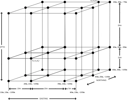
Within a single dimension, the spacing need not be constant. In Figure 1, Figure 2, and Figure 3, the spacings are constant, but Figure 6 below shows an example where this is not the case.

(28)

10m,10m,-100m 40m,30m,-100m 40m,20m,-100m 40m,10m,-100m 35m,10m,-100m 20m,10m,-100m 40m,30m,-90m 40m,30m,-70m EASTING NORTHING ` DEPTH 10m 15m 5m ` ` ` ` ` ` ` ` ` ` 20m 10m (t2,s2,p2) (t1,s1,p1)

Figure 6: A 3D grid showing real-world coordinates and nonuniformly-spaced points. In this case the grid spacing in the Northing dimension is constant (10 meters) but in the Easting and Depth dimensions the spacing varies. In Depth, the spacing is 20m and 10m; in Easting, the spacing is 10m, 15m, and 5m.

Conversion Between Grid Coordinates and Real-World Coordinates

The translation from grid coordinates to real-world coordinates can be viewed as a sequence of distinct operations:

1. Nonuniform grid spacing is applied (if appropriate). If the space between grid points in one or more dimensions isn’t constant, the nonuniform spacing is applied.

2. An affine transformation is applied. This process rotates and stretches the grid so that the grid axes coincide with real-world axes and the distance between grid points takes on the correct real-world values. 3. Finally, the origin of the grid (one of the corners) is shifted (translated)

(29)

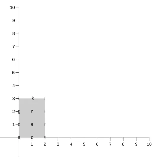
Figure 7 shows a simple 3x4 2D grid. The letters “a” through “l” are used to label the12 grid points.

9 1 2 3 4 5 6 7 8 9 10 1 8 7 6 5 4 3 2 10 h f b a g e k l j i d c

(30)

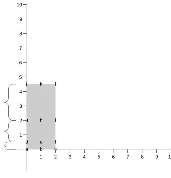
In Figure 8, nonuniform spacing on one of the axes has been applied. This changes the grid spacing from “1,1,1” to “.5, 1.5, 2.5.” Spacing on the other axis remains unchanged.

9 1 2 3 4 5 6 7 8 9 10 1 8 7 6 5 4 3 2 10 h f b a g e k l j i d c 2.5 1.5 0.5

(31)

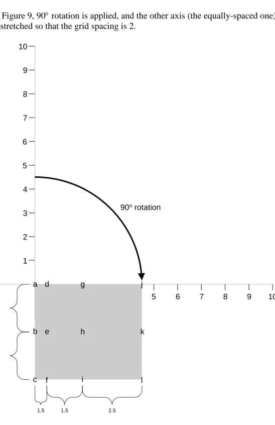
In Figure 9, 90 rotation is applied, and the other axis (the equally-spaced one) is stretched so that the grid spacing is 2.

9 1 2 3 4 5 6 7 8 9 10 1 8 7 6 5 4 3 2 10 2.5 1.5 1.5 g k l j d h i f e a b c 2.0 2.0 90o_rotation

(32)

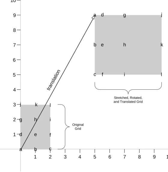
Finally, in Figure 10, the translation is applied, moving the original origin (the point labeled ‘a’( from point )0,0( to )5,9(.

9 1 2 3 4 5 6 7 8 9 10 1 8 7 6 5 4 3 2 10 g k l j d h i f e a b c h f b a g e k l j i d c Stretched, Rotated, and Translated Grid

Original Grid tra nsl atio n

Figure 10: Two views of the same grid – in grid coordinates and in real-world coordinates.

Data Values Are Attached to Grid Points

Just as data elements in an array are attached to array positions, or indices, data in grids are attached to the positions on the grids, called grid points. In Figure 6, for example, the (temperature, salinity, pressure) data triplets (t1, s1, p1) and (t2, s2, p2) are stored at the grid points corresponding to spatial positions (20m, 10m, -90m) and (35m, 30m, -70m), respectively.

(33)

One other feature that this example illustrates is that there can be more than one data element at each grid point – in this case there are three: temperature, salinity, and pressure. In this example, all the values are floating point, but in general some could be floating point, some could be integers, some could be text strings, etc. The BCS Grid Extension refers to these elements as variables. The Extension supports up to 102_{variables at each grid point, and the types of} the variables can be 8, 16, and 32 bit integers and 32 and 64 bit floating point numbers.

Some Grid Points Can Have Missing Values

It’s often the case that some of the variables at some of the grid points in a grid do not have recorded values. For example, if a grid represents the output of a vertical ocean sensor array over time, there may be some times when one of the sensors fails to record values. As some value must be stored for each variable in each grid position, there needs to be some means for indicating that a value appearing at some point in the grid “is not really there.” The strategies typically used include:

1. The FillValueapproach: a specific value )e.g., “0” or “-1”( is used to

indicate a missing value. The drawback of course is that real data having this value cannot be represented.

2. The NaN approach: IEEE floating point systems have special not-a-number values that are not used for any legitimate floating point numbers – unfortunately there is no equivalent for integer systems. 3. The BitMap approach: a boolean flag is associated with each grid point.

If the flag value is “true”, then the corresponding grid point value is considered to be valid; if the flag value is “false”, then the

corresponding grid point value is considered to be missing. This is the approach used in the BCS Grid Extension.

Extracting From Grids: Orthogonally, Radially, and Obliquely

A common operation on gridded data is to extract a portion of the data into a new grid. Note that:

 the new grid may have the same number of dimensions as the original

grid, or it may have fewer,

2

“10” is the value used in a compile-time constant used in the BCS Grid Extension code. There is no technical reason why the Extension could not be released with a larger value; this may be done in the future.

(34)

 an axis in the new grid may be parallel to an axis in the original grid, or it may not be,

 the grid points in the new grid may or may not coincide with grid points in the original grid, and

 the number of grid points in the new grid may be fewer than, the same

as, or more than the number of grid points in the original grid.

One form of extraction is a slice. Suppose air temperatures are stored in a 4D latitude/longitude/altitude/time grid and we are interested in how the air temperature at an altitude of 3000 meters varies with time and location. We might want to form a 3D latitude/longitude/time grid, keeping just the altitude values for the 3000-meter level. Other examples of slices are:

 a 2D latitude/longitude grid produced from, for example, all the data at an altitude of 1000 meters and a time of 3 hours,

 a 2D depth/time grid produced from, for example, temperature readings

at various ocean depths at a sequence of times3_{, and}

 a 1D time grid storing air temperature at a particular point in space as a function of time4_{. These are all examples of slices.}

Another form of extraction is a subset. Unlike a slice, a subset of a grid has the same number of dimensions as the original grid. Furthermore, the axes in the extracted grid coincide with the axes in the original grid, and the grid points in the extracted grid coincide with some of the grid points in the original grid. However, in a subset:

 the extent of one or more of the axes may be shorter than in the original grid, or

 the number of grid points along a dimension in the new grid may be

fewer than in the original grid.

Extractions can be classified as orthogonal, radial, or oblique.

3

This type of slice is also referred to as a profile.

4

(35)

Orthogonal Extractions

An orthogonal extraction is one where each of the axes in the extracted grid is parallel to some axis in the original grid. The latitude/longitude/altitude/time grid example discussed above illustrates orthogonal extractions. Figure 11 illustrates an orthogonal 3D grid (subset) taken from a larger 3D grid.

(36)

Radial Extractions

A radial extraction is an orthogonal extraction that has been rotated around one of the axes. Suppose we have a 3D latitude/longitude/depth grid. A typical operation is to extract several distance/depth grids centered around a particular latitude/longitude point, each grid (a radial slice or simply radial) radiating out from the point at a different angle (like spokes in a wheel). Figure 12 illustrates a radial extraction of three radial slices.

10m,10m,-100m 40m,30m,-100m 40m,20m,-100m 40m,10m,-100m 30m,10m,-100m 20m,10m,-100m 40m,30m,-99m 40m,30m,-98m EASTING NORTHING ` DEPTH

Original Grid Position Interpolated Grid Position 10m,10m,-98m

10m,10m,-100m

One of the three radial slices

(37)

Oblique Extraction

An oblique extraction is a non-radial extraction that has at least one axis that is not parallel with any of the axes in the original grid. Figure 13 illustrates such a slice. It also illustrates an extracted grid where most of the grid points do not lie on top of grid points in the original grid. The values at most of the grid points in the extracted grid are interpolated – see Interpolating Values at Grid Points on page 20 for a discussion of how this is done.

10m,10m,-100m 40m,30m,-100m 40m,20m,-100m 40m,10m,-100m 30m,10m,-100m 20m,10m,-100m 40m,30m,-99m 40m,30m,-98m EASTING NORTHING ` DEPTH

Original Grid Position Interpolated Grid Position 10m,20m,-99m 10m,20m,-99m 10m,20m,-99m 10m,20m,-99m 30m,30m,-99m 40m,20m,-99m 40m,20m,-98m 30m,30m,-98m

(38)

Interpolating Values at Grid Points

As discussed in the previous sections, the grid points in an extracted grid need not coincide with those of the parent (source) grid. When there is not an exact match between grid coordinates, as shown in the figure below, one of two sampling methods is used, as described in the following sections.

3 9 47 86 X 1 2 4 1 10 12 12 10 1

Figure 14: Interpolation between grid points.

Figure 14 illustrates a 2D grid with values defined at grid coordinates (1,1), )4,1(, )4,12(, and )1,12(. “X” marks a spot with grid coordinates )2,10(, for which there is no stored value.

The BCS Grid Extension supports the following interpolation schemes, and provides a mechanism to allow users to define their own schemes:

 n-linear interpolation,

 nearest-neighbor interpolation.

Nearest-Neighbor Interpolation

The simplest interpolation method is nearest-neighbor interpolation. This method is conceptually equivalent to snapping to the nearest grid point on the source grid. In the example shown above, the extracted grid value at X would be assigned the value 47, since X is closest to the grid cell containing 47.

N-linear Interpolation

The other method supported by the BCS Grid Extension is N-linear

interpolation. This method is a simple generalization of bi-linear interpolation. In the two-dimensional case shown, one would first linearly interpolate along one axis, as shown here:

(39)

P R O G R A M M E R ’ S G U I D E 3 9 47 86 X 5 60

Figure 15: N-linear interpolation.

and then linearly interpolate the interpolated values (5,60) to give a value of 505 at X.

Types of Dimensions

Measurement scales, and hence the dimensions of a grid, can be classified into four types6_:

nominal scales: values in the scale are unordered, and there is no notion of distance between values. Sex {male, female} is such a scale.

ordinal scales: values in the scale are ordered, but again there is no notion of distance between values. Educational attainment {high school (HS),

undergraduate degree (BSc), masters degree (MSc), doctorate (PhD)} is an ordinal scale. It is correct to say that on this scale PhD is higher than BSc, but it is not correct to say that the difference between BSc and MSc is the same as the difference between MSc and PhD. Nor is it correct to say that PhD equals 2 times BSc.

interval scales: values in the scale are ordered, and the difference between successive elements in the scale is constant. The Fahrenheit temperature scale is an interval scale. The difference in temperature between 40 and 50 is the same as the difference between 50 and 60, and it is true to say that 50 is hotter than 40. Note, however, that it is not correct to say that 50 is twice as hot as 25.

ratio scales: these are interval scales having an absolute zero. Not only is the difference between successive values significant, the ratio between values is significant as well. Salary is a ratio scale, as is the Kelvin temperature scale.

5

5 = 3 + (9-3)*(2-1)/(4-1); 60 = 47 + (86-47)*(2-1)/(4-1); 50 = 5 + (60-5)*(10-1)/(12-1).

6

(40)

The dimension scales used in a BCS Grid Extension grid can be of any of these four types7_{, although the type of scale will govern which types of interpolation} are reasonable. No type of interpolation is reasonable for a nominal scale, and nearest-neighbor is the only type of interpolation reasonable for an ordinal scale. Typically, some or all of the dimensions in a BCS Grid Extension grid are taken from the list {X, Y, altitude/depth, time}, all of which are ratio dimensions.

Projections and Other Mappings

Every point on the Earth has a unique {latitude, longitude, elevation} triplet of coordinates8_{, called its geographic coordinates. Computations of distance, area,} and direction using geographic coordinates are complicated, so it is often useful to introduce a mapping between geographic coordinates and a local Cartesian coordinate {northing, easting, elevation} system. This Cartesian coordinate system is known as a map projection. There are thousands of defined map projections, each one having certain beneficial properties and/or particular applicability in different parts of the world (e.g., equatorial areas, polar areas, etc.)

Another type of mapping is a grid rotation. As described in the NOAA publication

http://www.gfdl.noaa.gov/~smg/MOM/web/guide_parent/s4node18.html,

“this transform is particularly useful for studies of high latitude oceans where the convergence of lines of longitude may limit time steps or where the ocean contains a pole (as in the Arctic). The idea is to define a new grid in which the area of interest is far from the grid poles. In limited domain models, the pole can be rotated outside of the domain. For global models, one possibility is rotate the North Pole to

( W, N) which puts the North pole in Greenland

and keeps the South pole in Antarctica. Other uses include rotating the grid to match the angle of a coastline or to provide more flexibility in specifying lateral boundary conditions.”

Related to map projection is the concept of a spatial reference system. While a projection defines how to map cartesian coordinates to geographic coordinates, a spatial reference system defines how to map either cartesian coordinates or geographic coordinates to points on the Earth. A projection component of the

7

Including nominal, with the restriction that the data values must be numeric.

8

(41)

spatial reference system defines the mapping from cartesian coordinates to geographic coordinates, and datum and ellipsoid components define the mapping from geographic coordinates to points on the Earth. (For further information on spatial reference systems and the role of datum and ellipsoids, see Appendix G on page 237.)

For grids having spatial dimensions, the BCS Grid Extension allows the grid dimensions to be cast in terms of particular spatial reference systems

(geographic or projected). In addition, the Extension allows for grids stored with one spatial reference system to be converted to another spatial reference system on extraction.

Updating Grids

As with any other type of data residing in a database, it is often necessary to update grids. Types of updates can include:

 changing one or more of the values at individual grid points (Figure 16), Longitude Latitude Elevation t000 t100 t200 t300 t001 t310 t311 t101 t021 t121 t221 t321 t320 t000 t100 t200 t300 t001 t310 t311 t101 t021 t121 t'221 t321 t320

Figure 16: Updating temperature t

211 to t´211. All other values remain unchanged.

 adding onto the end of one of the dimensions, for example the time

dimension as data continues to be collected (Figure 17), and

Longitude

Time Elevation

0 1 2 3 4 0 1 2 3 4

(42)

 replacing an entire portion of a grid for a range of values in one or more of the dimensions (Figure 18).

Longitude Latitude Elevation Original Value New Value Original Grid Updated Grid New Grid Piece

Figure 18: Replacing a portion of a grid.

The BCS Grid Extension supports the third type of update, but both of the other two types of update can be framed as the update of a portion of a grid9_.

Aggregating Grids

By aggregating a grid, we mean constructing a new grid out of existing grids. Three types of grid aggregation10_are:

 JoinNew

 JoinExisting

 Union

9

For adding data onto the end of a dimension, this requires that the full grid first be pre-allocated with null data, which become updated with non-null data as they become available.

10

As defined by the OPeNDAP Aggregation Server (http://www.opendap.org/server/agg-html/agg_2.html).

(43)

JoinNew

The JoinNew form of aggregation is used to join grids along a new dimension, hence creating a grid of higher dimensionality. For example, Figure 19

illustrates the combining of a set of 2-dimensional (spatial) {X, Y} grids for successive time values into a single 3-dimensional {X, Y, time} grid.

Y X Time = 0 0 1 2 1 2 3 Y X Time = 4 0 1 2 1 2 3 Y X Time = 3 0 1 2 1 2 3 Y X Time = 2 0 1 2 1 2 3 Y X Time = 1 0 1 2 1 2 3 Y X Time 0 1 2 3 1 2 3 4

Figure 19: Combining {X,Y} grids for 5 different times into a single {X,Y,time} grid. The JoinNew form of aggregation is supported by the BCS Grid Extension GRDExtend / Update functionality. (See Chapter 6 on page 149.)

(44)

JoinExisting

The JoinExisting form of aggregation is used to consolidate grids that share the same axes and abut each other on one or more of these axes. For example, Figure 20 illustrates a JoinExisting aggregation between two {X,Y,time} grids.

1 2 Y X Time 0 1 2 3 1 2 3 4 1 2 Y X Time 4 5 6 1 2 3 4 0 0 X Time 0 1 2 3 1 2 3 4 1 2 Y 4 5 6

Figure 20: Merging XY grids for different time periods to form a single, longer grid. The JoinExisting form of aggregation is supported by the BCS Grid Extension

(45)

Union

The Union form of aggregation can be used to aggregate grids that have the same axes and cover the same spatio-temporal area, but have different

variables. Figure 21 shows the union aggregation of a salinity depth-time grid and a temperature depth-time grid.

s₀₀ s₂₁ s₁₁ s₀₁ s₂₀ s₁₀ depth time 0 1 0 1 2 s₀₂ s₂₃ s₁₃ s₀₃ s₂₂ s₁₂ 2 3 t₀₀ t₂₁ t₁₁ t₀₁ t₂₀ t₁₀ depth time 0 1 0 1 2 t₀₂ t₂₃ t₁₃ t₀₃ t₂₂ t₁₂ 2 3 depth time 1 0 2 3 s₀₀, t₀₀ s₂₁, t₂₁ s₁₁, t₁₁ s₁₀, t₁₀ 0 1 2 s₀₂, t₀₂ s₂₃, t₂₃ s₁₃, t₁₃ s₀₃, t₀₃ s₂₂, t₂₂ s₁₂, t₁₂ s₂₀, t₂₀ s₀₁, t₀₁

Figure 21: Unioning a salinity depth-time grid and a temperature depth-time grid to form a grid with both salinity and temperature.

The Union form of aggregation is supported by the BCS Grid Extension GRDValue/GRDUpdate functionality. (See Chapter 6 on page 149.)

(46)

Storing Grids in Files

Grids are used in many diverse applications; hence a number of different standards and formats have been defined for storing grids in files. Some of these are:

CDF (Common Data Format) is a library and toolkit for storing, manipulating,

and accessing multi-dimensional datasets. The basic component of CDF is a software interface that is a device-independent view of the CDF data model.

GRIB (GRIdded Binary) is the World Meteorological Organization (WMO)

standard for gridded meteorological data.

HDF (Hierarchical Data Format) is a self-defining file format for transfer of various types of data between different machines. The HDF library contains:

 interfaces for storing and retrieving compressed or uncompressed raster

images with palettes, and

 an interface for storing and retrieving n-dimensional scientific datasets together with information about the data, such as labels, units, formats, and scales for all dimensions.

netCDF (Network Common Data Form) is an interface for scientific data access that implements a machine-independent, self-describing, extensible file format.

SDTS (Spatial Data Transfer Standard) is a USA Federal standard (Federal

Information Processing Standard (FIPS) 173) for transfer of geologic and other spatial data.

DICOM (Digital Imaging and Communications in Medicine) has published a set of standards allowing for the storage and interchange of medical images and related information.

The BCS Grid Extension is packaged with an application that can import HDF, netCDF, GRIB, and DICOM files and save them in a BCS GRID Extension-enabled database. It can also import files served by OPeNDAP11_{servers. This} application is discussed in Appendix J on page 265.

11

(47)

The Role of Databases for Gridded Data

Until recently, gridded data was usually stored in files and users ran

applications on these files to generate the required data products. However, there is now increasing recognition that it is often advantageous to store gridded data in a modern database and allow users to extract data products by running queries against the database. Three advantages are as follows:

Uniform treatment of data items: By storing gridded data together with its metadata and other data, applications can use the simple SQL interface to perform complex queries based on any of these data items, including

dynamically-derived properties of the gridded data. An example of this would be the following pseudo-SQL query, which returns all pressures at a depth of 100 m, collected by a particular device:

SELECT GRDExtract(gridColumn, extractionSpecification) FROM tablename

WHERE inside(100, depth_range(gridColumn)) AND collection_device = “pressure_transducer”;

This basic query could be extended by modifying the text of the extraction specification to support more refined requests, such as selecting pressures collected during the last five hours, converting to a Lambert conformal

projection, etc. In contrast, gathering this information when the gridded data is on a file system would involve a complex application of not only queries but also code to locate, transform, and subset the relevant data.

Client-server issues: In a traditional database or file-based environment, custom functionality is implemented purely on the client side, resulting in “heavy clients”. Modern DBMSs, in addition to allowing user-defined types, also allow user-defined routines to be defined in languages such as C or Java, which provide much greater control over where functionality resides. Data can be assembled, processed and/or disassembled on either the client or the server, or both, with attendant tradeoffs.

Synchronized concurrent access to data: Multiple users of the database can safely query the same data simultaneously. With a file-based approach, there is a danger that the update activity of one application might result in another application seeing inconsistent data.

However, in order to realize the true potential of gridded databases, it is also necessary to provide for certain critical functionality to be available as an integrated component of the overall system. Some examples of disciplines requiring sophisticated operations were provided in the Application Areas for Gridded Data section (page 2).

(48)

Expanding on one of these examples, it is our experience that data products required by users of large grids often involve only very small portions of the grid. For instance, on a global weather grid, the region of interest may only be a few tens of kilometers on a side; on an oceanographic data grid, the required data might be a 2D slice 100 km long. Under these conditions, only a tiny fraction of the grid needs to be used to generate the products. Certain DBMSs can be made to perform such manipulations very efficiently through the use of tiling combined with blobs (binary large objects). By taking this approach, only those tiles that contain the data of interest are moved into memory during data product generation, and the vast majority of the gridded data is not involved in the data transfer or the computations. Understandably, this can be a very important performance consideration in the case of Web-based applications. As already noted, only certain types of DBMSs are suitable candidates for achieving all the potential advantages of using a database to store gridded data. In particular, object-relational DBMSs provide the support for UDTs (user-defined types) and UDRs (user-(user-defined routines) required to realize these advantages.

An Object-Relational Extension for Gridded

Data

Object-Relational Databases

Conventional relational database management systems support only a fixed set of data types, and these data types are usually fairly simple. For example, the 1992 SQL standard (SQL2) for relational database management systems supports the following data types: bit, bit varying, character, character varying, integer, floating point, arbitrary precision numeric, date, time, time interval, and binary large object.

In addition to the limitation in the variety of data types, SQL2 also restricts the operations on the data types to a limited, pre-defined set. For example, the integer data type supports operations like plus, minus, times, etc., but SQL2 provides no mechanism for defining new operations (say, for example, a “max2num” operation that takes two integers and returns the larger of them). For potentially large data elements such as pictures, sound recordings, and grids of data, SQL2 offers the “binary large object” )blob( data type. Unfortunately, there is very little that one can do with blobs; they can be inserted into a database and extracted from a database, but

 they cannot be used in the WHERE clause of queries:

(49)

 they cannot be used in the ORDER BY clause of queries:

e.g., “SELECT … ORDER BY blobcolumn;”

 they cannot be operated on in the SELECT clause of queries:

e.g., “SELECT func(blobcolumn( FROM …”

To address all of these concerns, object-relational database management systems allow a database designer to create user-defined types (UDTs) and

user-defined routines (UDRs) which operate on these types. With the

PostgreSQL object-relational database management system, a package of UDTs and UDRs designed to meet a class of business objectives is called an

Extension. The remainder of this chapter introduces the BCS Grid Extension, a package designed to assist in storing and manipulating gridded data in a PostgreSQL database.

The BCS Grid Extension – User-Defined Data Types

The BCS Grid Extension includes the following UDTs:

GRDValue: A GRDValue has two parts – a data component, containing gridded data, and a metadata component, containing the information needed to interpret that data (e.g., projection, dimensions, grid axis spacing, etc.). See The GRDValue Data Type on page 43 for a detailed discussion of the GRDValue data type.

GRDSpec: A GRDSpec contains the information necessary to extract a new grid from an existing GRDValue grid. Like a GRDValue, a GRDSpec also includes metadata. This metadata is used to override the metadata from the

original GRDValue. This means that a GRDSpec can direct that the extracted

GRDValue have different properties (e.g., size of axes, axis spacing, projection,

position of grid points) than the original GRDValue. See The GRDSpec Data

Typeon page 61 for a detailed discussion of the GRDSpec data type.

S-expression: Various classes of S-expressions (

http://en.wikipedia.org/wiki/S-expression) are used throughout the BCS Grid Extension; they provide a way of

bundling complex specifications into a single expression. These classes of S-expression are not actually implemented as UDTs but at a conceptual level they should be considered as data types, since many BCS Grid Extension SQL functions have string operands that take the form of S-expressions. See the table on page 202 for a detailed description of the various classes of S-expressions used in the BCS Grid Extension.

GRDBox: A GRDBox stores a grid’s bounding box in geocentric coordinates. GRDBox’s can be built from any GRDValue or GRDSpec that represents a real-world coordinate system (X, Y, depth/altitude, time) or (latitude, longitude, depth/altitude, time). The section Geolocating Grids: Finding Grids that Are in

(50)

a Particular Spatio-Temporal Location on page 143 describes how to use a GRDBox in a spatial index in order to find grids satisfying some

spatio-temporal criteria. (For example, find all grids that overlap some specified area, have altitude values between 8000 and 9000 meters, and have time values in the past 24 hours.)

GRDPriorityGrid and GRDFuseState: These types are used to resolve ambiguity when creating a composite grid from multiple, overlapping grids using grid fusion techniques. Grid fusion techniques are described in Aggregating Grids: Grid Fusion on page 137.

The BCS Grid Extension – User-Defined Routines

The BCS Grid Extension includes over forty functions for creating,

manipulating, and extracting grids of data. A complete description of these functions is provided in Appendix A on page 199.

The set of BCS Grid Extension functions includes:

 functions for creating GRDBox’s, GRDSpec’s, GRDValue’s, and

GRDPriorityGrid’s,

 functions for querying the metadata portion of a GRDValue,

 functions for extracting GRDValue’s,

 functions for manipulating and updating GRDValue’s, and

(51)

Chapter 2: Installing the

BCS Grid Extension

This chapter describes how to install the BCS Grid Extension software onto a Linux server machine and perform some simple operations to test the

installation.

Installing the Software

The BCS Grid Extension requires that an appropriate version of the

PostgreSQL server already be installed on the target machine. Currently the BCS Grid Extension is tested to run under PostgreSQL version 8.4. If you are running a different version of PostgreSQL, please contact BCS for a custom version of the BCS Grid Extension.

The first step in the installation process is to log in as root. This can be done by either logging on as root at a login prompt or running the “su -” command to start a shell as the root user12_.

The second step is to execute the install package. The install package's name is of the form

bcsgrid-*-postgresql-*-linux.bin (regular version)

or

bcsgrid-*-postgresql-*-linux.Expires_on.yyyy-mm-dd.bin (evaluation version)

12

Note that the '-' argument to su is necessary. Without the '-' argument, the su command will not execute the root's profile, and hence the install package would be unable to find commands it needs.

Chapter

(52)

where the first * is replaced by the version of the BCS Grid Extension, and the second * is replaced by the version of the bundled PostgreSQL distribution. For evaluation versions, yyyy-mm-dd refers to the evaluation expiry year, month, and day.

To install BCS Grid Extension version 5.3.2.0 with PostgreSQL version 8.4.8 you would execute the following statements:

chmod u+x bcsgrid-5.3.2.0-postgresql-8.4.8-linux.bin ./bcsgrid-5.3.2.0-postgresql-8.4.8-linux.bin

The install package provides a series of explanatory messages and prompts to assist a user in configuring a new installation. The explanatory messages are rather long, and so are not reproduced here, but sample prompts are shown below.

Beginning installation...

PostgreSQL appears to be installed and running in /usr/lib/postgresql/8.4/bin

Enter the port used by PostgreSQL [5432] > Enter a directory for the initial blobspace [/opt/postgres/BLOBSPACE] >

Enter a database name [bcsgrid] > Is this correct? y/[n] >

Note that the BCS Grid Extension will write error messages into the

“serverlog” file in the PostgreSQL data directory specified in the installation. Two PostgreSQL-related environment variables can optionally be set to make starting psql, the PostgreSQL SQL client program, more convenient. The variables are PGDATABASE and PGUSER. PGDATABASE selects the database that will be connected to if no database is otherwise specified. PGUSER selects the user id that the connection will be associated with if no user id is otherwise specified13_{. Setting these variables removes the need to pass the database name} and username to psql as command line arguments.

13_If_PGUSER_{is not set and no userid is specified in the command line arguments to psql, then the} PostgreSQL userid will default to the Linux userid.

(53)

Setting Up the License Key

A license key is needed for each computer on which the PostgreSQL server runs. The license key is provided to the BCS Grid Extension by adding the following lines to the .bashrc file in the postgres account14_:

export GRID_LICENSE_KEY

GRID_LICENSE_KEY=license_key_value

If there is a line in the file that reads

# User specific aliases and functions place the license key statements right below that line.

Next, restart the PostgreSQL server. A simple way to do this is to log into the root account, cd to the /etc/init.d directory and execute the following commands:

./postgresql15_stop

./postgresql start

The license key is dependent on your machine's hostname and ip address. If either of these change, you will need to contact Barrodale Computing Services Ltd. for a new license key.

14

If the postgres account runs with some shell other than bash, then the means for setting the GRID_LICENSE_KEY environment variable will be different. For example, if csh or tcsh is used, then “setenv GRID_LICENSE_KEY license_key_value” will need to be placed in the .cshrc file in the postgres account.

15

The exact name of the command may differ. For example, under Ubuntu with PostgreSQL 8.4 the command is called “postgresql-8.4”

(54)

Testing the Installation

This section leads the reader through creating a table, populating it, and doing an extraction. In the following example, ‘$’ represents the Unix command line prompt and ‘bcsgrid=#’ represents the psql prompt16_{. Note that the following} example is not a realistic example of the use of the BCS Grid Extension. However, it does illustrate some core functionality of the Extension.

In this example, a simple 2D grid is created. The axes are each 1 unit (2 grid points) long and the four grid points have values as shown below:

1.0 .5 .5 1.0 Value = 5 Value = 5 Value = 0 Value = 10

Figure 22: Original 2D 2x2 grid.

The grid is created by first initializing an empty grid (using the

GRDValueFromSExpr function), then editing the external representation of the grid, and reloading the grid into the database17_{. A 1D diagonal slice is then} produced as shown in the following diagram:

16

The string preceding the =# (in this case bcsgrid) is the database name. 17

That is one of the “unrealistic” parts foretold earlier. The Extension user would instead use one of the Extension UDRs to populate the grid table from an external file.

(55)

P R O G R A M M E R ’ S G U I D E 1.0 .5 .5 1.0 0 8 7 5 6 4 3 2 1 9 10 New 1D Grid

Figure 23: Final 1D grid with 11 grid points.

The following sections proceed through this example, one step at a time. C R E A T E A N D L O A D A T A B L E

Execute the following Unix and psql commands18_: $ psql bcsgrid

In the following “create table” command, the S-expression '((srid -1)(dim_sizes 2 2 1 1)(dim_names x y dum1

dum2)(tile_sizes 2 2 1 1))' represents a grid with:

 spatial reference system id -1,

 dimensions of 2x2x1x1 (effectively a 2x2 grid with 2

grid points in each dimension), and

 axis names “x” and “y.” )The two empty grid

dimensions have names “dum1” and “dum2.”( bcsgrid=# CREATE TABLE testtab(namelist text[],