ElasticTree: Saving Energy in Data Center Networks
Brandon Heller
⋆, Srini Seetharaman
†, Priya Mahadevan
⋄,
Yiannis Yiakoumis
⋆, Puneet Sharma
⋄, Sujata Banerjee
⋄, Nick McKeown
⋆ ⋆ Stanford University, Palo Alto, CA USA† Deutsche Telekom R&D Lab, Los Altos, CA USA ⋄ Hewlett-Packard Labs, Palo Alto, CA USA
ABSTRACT
Networks are a shared resource connecting critical IT in-frastructure, and the general practice is toalways leave them on. Yet, meaningful energy savings can result from improving a network’s ability to scale up and down, as traffic demands ebb and flow. We presentElasticTree, a network-wide power1 manager, which dynamically ad-justs the set of active network elements — links and switches — to satisfy changing data center traffic loads.
We first compare multiple strategies for finding minimum-power network subsets across a range of traf-fic patterns. We implement and analyze ElasticTree on a prototype testbed built with production OpenFlow switches from three network vendors. Further, we ex-amine the trade-offs between energy efficiency, perfor-mance and robustness, with real traces from a produc-tion e-commerce website. Our results demonstrate that for data center workloads, ElasticTree can save up to 50% of network energy, while maintaining the ability to handle traffic surges. Our fast heuristic for computing network subsets enables ElasticTree to scale to data cen-ters containing thousands of nodes. We finish by show-ing how a network admin might configure ElasticTree to satisfy their needs for performance and fault tolerance, while minimizing their network power bill.
1.
INTRODUCTION
Data centers aim to provide reliable and scalable computing infrastructure for massive Internet ser-vices. To achieve these properties, they consume huge amounts of energy, and the resulting opera-tional costs have spurred interest in improving their efficiency. Most efforts have focused on servers and cooling, which account for about 70% of a data cen-ter’s total power budget. Improvements include bet-ter components (low-power CPUs [12], more effi-cient power supplies and water-cooling) as well as better software (tickless kernel, virtualization, and smart cooling [30]).
With energy management schemes for the largest power consumers well in place, we turn to a part of the data center that consumes 10-20% of its total
1
We use power and energy interchangeably in this paper.
power: the network [9]. The total power consumed by networking elements in data centers in 2006 in the U.S. alone was 3 billion kWh and rising [7]; our goal is to significantly reduce this rapidly growing energy cost.
1.1
Data Center Networks
As services scale beyond ten thousand servers, inflexibility and insufficient bisection bandwidth have prompted researchers to explore alternatives to the traditional 2N tree topology (shown in Fig-ure 1(a)) [1] with designs such as VL2 [10], Port-Land [24], DCell [16], and BCube [15]. The re-sulting networks look more like a mesh than a tree. One such example, the fat tree [1]2, seen in Figure 1(b), is built from a large number of richly connected switches, and can support any communication pat-tern (i.e. full bisection bandwidth). Traffic from lower layers is spread across the core, using multi-path routing, valiant load balancing, or a number of other techniques.
In a 2N tree, one failure can cut the effective bi-section bandwidth in half, while two failures can dis-connect servers. Richer, mesh-like topologies handle failures more gracefully; with more components and more paths, the effect of any individual component failure becomes manageable. This property can also help improve energy efficiency. In fact, dynamically varying the number of active (powered on) network elements provides a control knob to tune between energy efficiency, performance, and fault tolerance, which we explore in the rest of this paper.
1.2
Inside a Data Center
Data centers are typically provisioned for peak workload, and run well below capacity most of the time. Traffic varies daily (e.g., email checking during the day), weekly (e.g., enterprise database queries on weekdays), monthly (e.g., photo sharing on holi-days), and yearly (e.g., more shopping in December). Rare events like cable cuts or celebrity news may hit the peak capacity, but most of the time traffic can be satisfied by a subset of the network links and
2
(a) Typical Data Center Network. Racks hold up to 40 “1U” servers, and two edge switches (i.e.“top-of-rack” switches.)
(b) Fat tree. All 1G links, always on. (c) Elastic Tree. 0.2 Gbps per host across data center can be satisfied by a fat tree subset (here, a spanning tree), yielding 38% savings.
Figure 1: Data Center Networks: (a), 2N Tree(b), Fat Tree (c), ElasticTree
0 5 10 15 20 0 100 200 300 400 500 600 700 800 0 1000 2000 3000 4000 5000 6000 7000 8000
Bandwidth in Gbps Power in Watts
Time (1 unit = 10 mins) Total Traffic in Gbps
Power Traffic
Figure 2: E-commerce website: 292 produc-tion web servers over 5 days. Traffic varies by day/weekend, power doesn’t.
switches. These observations are based on traces collected from two production data centers.
Trace 1 (Figure 2) shows aggregate traffic col-lected from 292 servers hosting an e-commerce ap-plication over a 5 day period in April 2008 [22]. A clear diurnal pattern emerges; traffic peaks during the day and falls at night. Even though the traffic varies significantly with time, the rack and aggre-gation switches associated with these servers draw constant power (secondary axis in Figure2).
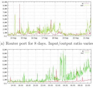
Trace 2 (Figure3) shows input and output traffic at a router port in a production Google data center in September 2009. The Y axis is in Mbps. The 8-day trace shows diurnal and weekend/week8-day vari-ation, along with a constant amount of background traffic. The 1-day trace highlights more short-term bursts. Here, as in the previous case, the power consumed by the router is fixed, irrespective of the traffic through it.
1.3
Energy Proportionality
An earlier power measurement study [22] had pre-sented power consumption numbers for several data center switches for a variety of traffic patterns and
(a) Router port for 8 days. Input/output ratio varies.
(b) Router port from Sunday to Monday. Note marked increase and short-term spikes.
Figure 3: Google Production Data Center
switch configurations. We use switch power mea-surements from this study and summarize relevant results in Table1. In all cases, turning the switch on consumes most of the power; going from zero to full traffic increases power by less than 8%. Turning off a switch yields the most power benefits, while turning off an unused port saves only 1-2 Watts. Ideally, an unused switch would consume no power, and energy usage would grow with increasing traffic load. Con-suming energy in proportion to the load is a highly desirable behavior [4,22].
Unfortunately, today’s network elements are not energy proportional: fixed overheads such as fans, switch chips, and transceivers waste power at low loads. The situation is improving, as competition encourages more efficient products, such as closer-to-energy-proportional links and switches [19, 18,
Ports Port Model A Model B Model C Enabled Traffic power (W) power (W) power (W)
None None 151 133 76
All None 184 170 97
All 1 Gbps 195 175 102
Table 1: Power consumption of various 48-port switches for different configurations
combination of improved components and improved component management.
Our choice – as presented in this paper – is to manage today’s non energy-proportional network components more intelligently. By zooming out to a whole-data-center view, a network of on-or-off, non-proportional components can act as an energy-proportional ensemble, and adapt to varying traffic loads. The strategy is simple: turn off the links and switches that we don’t need, right now, to keep avail-able only as much networking capacity as required.
1.4
Our Approach
ElasticTree is a network-wide energy optimizer that continuously monitors data center traffic con-ditions. It chooses the set of network elements that must stay active to meet performance and fault tol-erance goals; then it powers down as many unneeded links and switches as possible. We use a variety of methods to decide which subset of links and switches to use, including a formal model, greedy bin-packer, topology-aware heuristic, and prediction methods. We evaluate ElasticTree by using it to control the network of a purpose-built cluster of computers and switches designed to represent a data center. Note that our approach applies to currently-deployed net-work devices, as well as newer, more energy-efficient ones. It applies to single forwarding boxes in a net-work, as well as individual switch chips within a large chassis-based router.
While the energy savings from powering off an individual switch might seem insignificant, a large data center hosting hundreds of thousands of servers will have tens of thousands of switches deployed. The energy savings depend on the traffic patterns, the level of desired system redundancy, and the size of the data center itself. Our experiments show that, on average, savings of 25-40% of the network en-ergy in data centers is feasible. Extrapolating to all data centers in the U.S., we estimate the savings to be about 1 billion KWhr annually (based on 3 bil-lion kWh used by networking devices in U.S. data centers [7]). Additionally, reducing the energy con-sumed by networking devices also results in a pro-portional reduction in cooling costs.
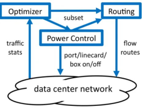
Figure 4: System Diagram
The remainder of the paper is organized as fol-lows: §2 describes in more detail the ElasticTree approach, plus the modules used to build the pro-totype. §3 computes the power savings possible for different communication patterns to understand best and worse-case scenarios. We also explore power savings using real data center traffic traces. In §4, we measure the potential impact on bandwidth and latency due to ElasticTree. In§5, we explore deploy-ment aspects of ElasticTree in a real data center. We present related work in §6 and discuss lessons learned in§7.
2.
ELASTICTREE
ElasticTree is a system for dynamically adapting the energy consumption of a data center network. ElasticTree consists of three logical modules - opti-mizer, routing, and power control - as shown in Fig-ure4. The optimizer’s role is to find the minimum-power network subset which satisfies current traffic conditions. Its inputs are the topology, traffic ma-trix, a power model for each switch, and the desired fault tolerance properties (spare switches and spare capacity). The optimizer outputs a set of active components to both the power control and routing modules. Power control toggles the power states of ports, linecards, and entire switches, while routing chooses paths for all flows, then pushes routes into the network.
We now show an example of the system in action.
2.1
Example
Figure1(c)shows a worst-case pattern for network locality, where each host sends one data flow halfway across the data center. In this example, 0.2 Gbps of traffic per host must traverse the network core. When the optimizer sees this traffic pattern, it finds which subset of the network is sufficient to satisfy the traffic matrix. In fact, a minimum spanning tree (MST) is sufficient, and leaves 0.2 Gbps of extra capacity along each core link. The optimizer then
informs the routing module to compress traffic along the new sub-topology, and finally informs the power control module to turn off unneeded switches and links. We assume a 3:1 idle:active ratio for modeling switch power consumption; that is, 3W of power to have a switch port, and 1W extra to turn it on, based on the 48-port switch measurements shown in Table
1. In this example, 13/20 switches and 28/48 links stay active, and ElasticTree reduces network power by 38%.
As traffic conditions change, the optimizer con-tinuously recomputes the optimal network subset. As traffic increases, more capacity is brought online, until the full network capacity is reached. As traffic decreases, switches and links are turned off. Note that when traffic is increasing, the system must wait for capacity to come online before routing through that capacity. In the other direction, when traffic is decreasing, the system must change the routing - by moving flows off of soon-to-be-down links and switches - before power control can shut anything down.
Of course, this example goes too far in the direc-tion of power efficiency. The MST soludirec-tion leaves the network prone to disconnection from a single failed link or switch, and provides little extra capacity to absorb additional traffic. Furthermore, a network operated close to its capacity will increase the chance of dropped and/or delayed packets. Later sections explore the tradeoffs between power, fault tolerance, and performance. Simple modifications can dramat-ically improve fault tolerance and performance at low power, especially for larger networks. We now describe each of ElasticTree modules in detail.
2.2
Optimizers
We have developed a range of methods to com-pute a minimum-power network subset in Elastic-Tree, as summarized in Table2. The first method is a formal model, mainly used to evaluate the solution quality of other optimizers, due to heavy computa-tional requirements. The second method is greedy bin-packing, useful for understanding power savings for larger topologies. The third method is a simple heuristic to quickly find subsets in networks with regular structure. Each method achieves different tradeoffs between scalability and optimality. All methods can be improved by considering a data cen-ter’s past traffic history (details in§5.4).
2.2.1
Formal Model
We desire the optimal-power solution (subset and flow assignment) that satisfies the traffic constraints,
3
Bounded percentage from optimal, configured to 10%.
Type Quality Scalability Input Topo
Formal Optimal3
Low Traffic Matrix Any
Greedy Good Medium Traffic Matrix Any
Topo- OK High Port Counters Fat
aware Tree
Table 2: Optimizer Comparison
but finding the optimal flow assignment alone is an NP-complete problem for integer flows. Despite this computational complexity, the formal model pro-vides a valuable tool for understanding the solution quality of other optimizers. It is flexible enough to support arbitrary topologies, but can only scale up to networks with less than 1000 nodes.
The model starts with a standard multi-commodity flow (MCF) problem. For the precise MCF formulation, see Appendix A. The constraints include link capacity, flow conservation, and demand satisfaction. The variables are the flows along each link. The inputs include the topology, switch power model, and traffic matrix. To optimize for power, we add binary variables for every link and switch, and constrain traffic to only active (powered on) links and switches. The model also ensures that the full power cost for an Ethernet link is incurred when ei-ther side is transmitting; ei-there is no such thing as a half-on Ethernet link.
The optimization goal is to minimize the total net-work power, while satisfying all constraints. Split-ting a single flow across multiple links in the topol-ogy might reduce power by improving link utilization overall, but reordered packets at the destination (re-sulting from varying path delays) will negatively im-pact TCP performance. Therefore, we include con-straints in our formulation to (optionally) prevent flows from getting split.
The model outputs a subset of the original topol-ogy, plus the routes taken by each flow to satisfy the traffic matrix. Our model shares similar goals to Chabareket al.[6], which also looked at power-aware routing. However, our model (1) focuses on data centers, not wide-area networks, (2) chooses a sub-set of a fixed topology, not the component (switch) configurations in a topology, and (3) considers indi-vidual flows, rather than aggregate traffic.
We implement our formal method using both MathProg and General Algebraic Modeling System (GAMS), which are high-level languages for opti-mization modeling. We use both the GNU Linear Programming Kit (GLPK) and CPLEX to solve the formulation.
2.2.2
Greedy Bin-Packing
For even simple traffic patterns, the formal model’s solution time scales to the 3.5thpower as a
function of the number of hosts (details in§5). The greedy bin-packing heuristic improves on the formal model’s scalability. Solutions within a bound of opti-mal are not guaranteed, but in practice, high-quality subsets result. For each flow, the greedy bin-packer evaluates possible paths and chooses the leftmost one with sufficient capacity. By leftmost, we mean in reference to a single layer in a structured topol-ogy, such as a fat tree. Within a layer, paths are chosen in a deterministic left-to-right order, as op-posed to a random order, which would evenly spread flows. When all flows have been assigned (which is not guaranteed), the algorithm returns the active network subset (set of switches and links traversed by some flow) plus each flow path.
For some traffic matrices, the greedy approach will not find a satisfying assignment for all flows; this is an inherent problem with any greedy flow assign-ment strategy, even when the network is provisioned for full bisection bandwidth. In this case, the greedy search will have enumerated all possible paths, and the flow will be assigned to the path with the lowest load. Like the model, this approach requires knowl-edge of the traffic matrix, but the solution can be computed incrementally, possibly to support on-line usage.
2.2.3
Topology-aware Heuristic
The last method leverages the regularity of the fat tree topology to quickly find network subsets. Unlike the other methods, it does not compute the set of flow routes, and assumes perfectly divisible flows. Of course, by splitting flows, it will pack every link to full utilization and reduce TCP bandwidth — not exactly practical.
However, simple additions to this “starter sub-set” lead to solutions of comparable quality to other methods, but computed with less information, and in a fraction of the time. In addition, by decoupling power optimization from routing, our method can be applied alongsideany fat tree routing algorithm, including OSPF-ECMP, valiant load balancing [10], flow classification [1] [2], and end-host path selec-tion [23]. Computing this subset requires only port counters, not a full traffic matrix.
The intuition behind our heuristic is that to satisfy traffic demands, an edge switch doesn’t care which
aggregation switches are active, but instead, how manyare active. The “view” of every edge switch in a given pod is identical; all see the same number of aggregation switches above. The number of required
switches in the aggregation layer is then equal to the number of links required to support the traffic of the most active source above or below (whichever is higher), assuming flows are perfectly divisible. For example, if the most active source sends 2 Gbps of traffic up to the aggregation layer and each link is 1 Gbps, then two aggregation layer switches must stay on to satisfy that demand. A similar observa-tion holds between each pod and the core, and the exact subset computation is described in more detail in§5. One can think of the topology-aware heuristic as a cron job for that network, providing periodic input toany fat tree routing algorithm.
For simplicity, our computations assume a homo-geneous fat tree with one link between every con-nected pair of switches. However, this technique applies to full-bisection-bandwidth topologies with any number of layers (we show only 3 stages), bun-dled links (parallel links connecting two switches), or varying speeds. Extra “switches at a given layer” computations must be added for topologies with more layers. Bundled links can be considered sin-gle faster links. The same computation works for other topologies, such as the aggregated Clos used by VL2 [10], which has 10G links above the edge layer and 1G links to each host.
We have implemented all three optimizers; each outputs a network topology subset, which is then used by the control software.
2.3
Control Software
ElasticTree requires two network capabilities: traffic data (current network utilization) and control over flow paths. NetFlow [27], SNMP and sampling can provide traffic data, while policy-based rout-ing can provide path control, to some extent. In our ElasticTree prototype, we use OpenFlow [29] to achieve the above tasks.
OpenFlow: OpenFlow is an open API added to commercial switches and routers that provides a flow table abstraction. We first use OpenFlow to validate optimizer solutions by directly pushing the computed set of application-level flow routes to each switch, then generating traffic as described later in this section. In the live prototype, OpenFlow also provides the traffic matrix (flow-specific counters), port counters, and port power control. OpenFlow enables us to evaluate ElasticTree on switches from different vendors, with no source code changes.
NOX: NOX is a centralized platform that pro-vides network visibility and control atop a network of OpenFlow switches [13]. The logical modules in ElasticTree are implemented as a NOX applica-tion. The application pulls flow and port counters,
Figure 5: Hardware Testbed (HP switch for
k= 6 fat tree)
Vendor Model k Virtual Switches Ports Hosts
HP 5400 6 45 270 54
Quanta LB4G 4 20 80 16
NEC IP8800 4 20 80 16
Table 3: Fat Tree Configurations
directs these to an optimizer, and then adjusts flow routes and port status based on the computed sub-set. In our current setup, we do not power off in-active switches, due to the fact that our switches are virtual switches. However, in a real data cen-ter deployment, we can leverage any of the existing mechanisms such as command line interface, SNMP or newer control mechanisms such as power-control over OpenFlow in order to support the power control features.
2.4
Prototype Testbed
We build multiple testbeds to verify and evaluate ElasticTree, summarized in Table3, with an exam-ple shown in Figure 5. Each configuration multi-plexes many smaller virtual switches (with 4 or 6 ports) onto one or more large physical switches. All communication between virtual switches is done over direct links (not through any switch backplane or in-termediate switch).
The smaller configuration is a complete k = 4 three-layer homogeneous fat tree4, split into 20 in-dependent four-port virtual switches, supporting 16 nodes at 1 Gbps apiece. One instantiation com-prised 2 NEC IP8800 24-port switches and 1 48-port switch, running OpenFlow v0.8.9 firmware pro-vided by NEC Labs. Another comprised two Quanta LB4G 48-port switches, running the OpenFlow Ref-erence Broadcom firmware.
4
Refer [1] for details on fat trees and definition ofk
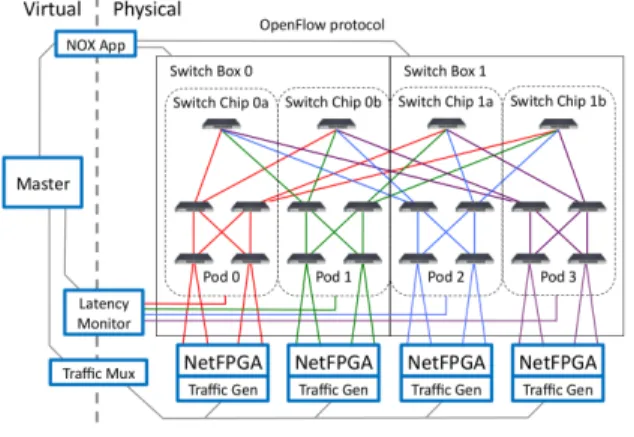
Figure 6: Measurement Setup
The larger configuration is a complete k = 6 three-layer fat tree, split into 45 independent six-port virtual switches, supsix-porting 54 hosts at 1 Gbps apiece. This configuration runs on one 288-port HP ProCurve 5412 chassis switch or two 144-port 5406 chassis switches, running OpenFlow v0.8.9 firmware provided by HP Labs.
2.5
Measurement Setup
Evaluating ElasticTree requires infrastructure to generate a small data center’s worth of traffic, plus the ability to concurrently measure packet drops and delays. To this end, we have implemented a NetF-PGA based traffic generator and a dedicated latency monitor. The measurement architecture is shown in Figure 6.
NetFPGA Traffic Generators. The NetFPGA Packet Generator provides deterministic, line-rate traffic generation for all packet sizes [28]. Each NetFPGA emulates four servers with 1GE connec-tions. Multiple traffic generators combine to emulate a larger group of independent servers: for the k=6 fat tree, 14 NetFPGAs represent 54 servers, and for the k=4 fat tree,4 NetFPGAs represent 16 servers.
At the start of each test, the traffic distribu-tion for each port is packed by a weighted round robin scheduler into the packet generator SRAM. All packet generators are synchronized by sending one packet through an Ethernet control port; these con-trol packets are sent consecutively to minimize the start-time variation. After sending traffic, we poll and store the transmit and receive counters on the packet generators.
Latency Monitor. The latency monitor PC sends tracer packets along each packet path. Tracers enter and exit through a different port on the same physical switch chip; there is one Ethernet port on the latency monitor PC per switch chip. Packets are
logged by Pcap on entry and exit to record precise timestamp deltas. We report median figures that are averaged over all packet paths. To ensure measure-ments are taken in steady state, the latency moni-tor starts up after 100 ms. This technique captures all but the last-hop egress queuing delays. Since edge links are never oversubscribed for our traffic patterns, the last-hop egress queue should incur no added delay.
3.
POWER SAVINGS ANALYSIS
In this section, we analyze ElasticTree’s network energy savings when compared to an always-on base-line. Our comparisons assume a homogeneous fat tree for simplicity, though the evaluation also applies to full-bisection-bandwidth topologies with aggrega-tion, such as those with 1G links at the edge and 10G at the core. The primary metric we inspect is
% original network power, computed as:
= Power consumed by ElasticTree×100 Power consumed by original fat-tree This percentage gives an accurate idea of the over-all power saved by turning off switches and links (i.e., savings equal 100 - % original power). We use power numbers from switch model A (§1.3) for both the baseline and ElasticTree cases, and only include active (powered-on) switches and links for ElasticTree cases. Since all three switches in Ta-ble 1 have an idle:active ratio of 3:1 (explained in §2.1), using power numbers from switch model B or C will yield similar network energy savings. Un-less otherwise noted, optimizer solutions come from the greedy bin-packing algorithm, with flow splitting disabled (as explained in Section2). We validate the results for allk={4,6}fat tree topologies on mul-tiple testbeds. For all communication patterns, the measured bandwidth as reported by receive counters matches the expected values. We only report energy saved directly from the network; extra energy will be required to power on and keep running the servers hosting ElasticTree modules. There will be addi-tional energy required for cooling these servers, and at the same time, powering off unused switches will result in cooling energy savings. We do not include these extra costs/savings in this paper.
3.1
Traffic Patterns
Energy, performance and robustness all depend heavily on the traffic pattern. We now explore the possible energy savings over a wide range of commu-nication patterns, leaving performance and robust-ness for§4.
0.0
0.2
Traffic Demand (Gbps)
0.4
0.6
0.8
1.0
0
20
40
60
80
100
% original network power
Far
50% Far, 50% Mid Mid
50% Near, 50% Mid Near
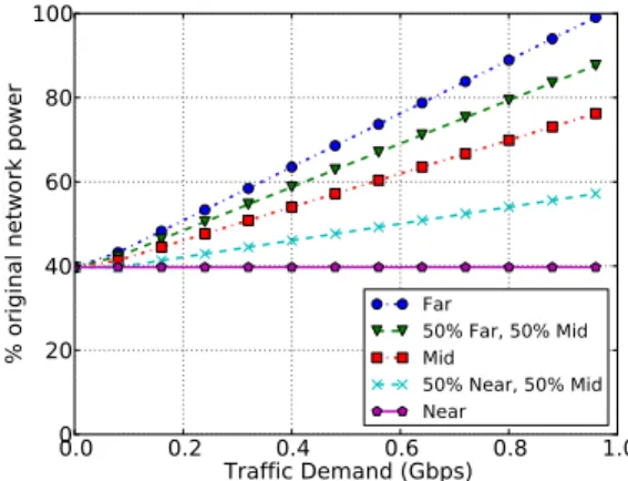
Figure 7: Power savings as a function of de-mand, with varying traffic locality, for a 28K-node, k=48 fat tree
3.1.1
Uniform Demand, Varying Locality
First, consider two extreme cases: near (highly localized) traffic matrices, where servers commu-nicate only with other servers through their edge switch, and far (non-localized) traffic matrices where servers communicate only with servers in other pods, through the network core. In this pat-tern, all traffic stays within the data center, and none comes from outside. Understanding these ex-treme cases helps to quantify the range of network energy savings. Here, we use the formal method as the optimizer in ElasticTree.
Neartraffic is a best-case — leading to the largest energy savings — because ElasticTree will reduce the network to the minimum spanning tree, switch-ing off all but one core switch and one aggregation switch per pod. On the other hand, far traffic is a worst-case — leading to the smallest energy savings — because every link and switch in the network is needed. For far traffic, the savings depend heavily on the network utilization,u=
P
i
P
jλij
Total hosts (λij is the
traffic from hosti to hostj, λij <1 Gbps). If uis
close to 100%, then all links and switches must re-main active. However, with lower utilization, traffic can be concentrated onto a smaller number of core links, and unused ones switch off. Figure 7 shows the potential savings as a function of utilization for both extremes, as well as traffic to the aggregation layerMid), for a k= 48 fat tree with roughly 28K servers. Running ElasticTree on this configuration, withnear traffic at low utilization, we expect a net-work energy reduction of 60%; we cannot save any further energy, as the active network subset in this case is the MST. Forfar traffic andu=100%, there are no energy savings. This graph highlights the power benefit of local communications, but more
im-0.0 0.1 0.2 0.3 0.4 0.5 0.6 0.7 Avg. network utilization
0 20 40 60 80 100
% original network power
Figure 8: Scatterplot of power savings with random traffic matrix. Each point on the graph corresponds to a pre-configured aver-age data center workload, for ak= 6 fat tree
portantly, shows potential savings in all cases. Hav-ing seen these two extremes, we now consider more realistic traffic matrices with a mix of bothnearand
far traffic.
3.1.2
Random Demand
Here, we explore how much energy we can expect to save, on average, with random, admissible traf-fic matrices. Figure 8 shows energy saved by Elas-ticTree (relative to the baseline) for these matrices, generated by picking flows uniformly and randomly, then scaled down by the most oversubscribed host’s traffic to ensure admissibility. As seen previously, for low utilization, ElasticTree saves roughly 60% of the network power, regardless of the traffic matrix. As the utilization increases, traffic matrices with sig-nificant amounts offartraffic will have less room for power savings, and so the power saving decreases. The two large steps correspond to utilizations at which an extra aggregation switch becomes neces-sary across all pods. The smaller steps correspond to individual aggregation or core switches turning on and off. Some patterns will densely fill all available links, while others will have to incur the entire power cost of a switch for a single link; hence the variabil-ity in some regions of the graph. Utilizations above 0.75 are not shown; for these matrices, the greedy bin-packer would sometimes fail to find a complete satisfying assignment of flows to links.
3.1.3
Sine-wave Demand
As seen before (§1.2), the utilization of a data cen-ter will vary over time, on daily, seasonal and annual
Figure 9: Power savings for sinusoidal traffic variation in a k= 4 fat tree topology, with 1 flow per host in the traffic matrix. The input demand has 10 discrete values.
time scales. Figure 9 shows a time-varying utiliza-tion; power savings from ElasticTree that follow the utilization curve. To crudely approximate diurnal variation, we assume u= 1/2(1 + sin(t)), at timet, suitably scaled to repeat once per day. For this sine wave pattern of traffic demand, the network power can be reduced up to 64% of the original power con-sumed, without being over-subscribed and causing congestion.
We note that most energy savings in all the above communication patterns comes from powering off switches. Current networking devices are far from being energy proportional, with even completely idle switches (0% utilization) consuming 70-80% of their fully loaded power (100% utilization) [22]; thus pow-ering off switches yields the most energy savings.
3.1.4
Traffic in a Realistic Data Center
In order to evaluate energy savings with a real data center workload, we collected system and net-work traces from a production data center hosting an e-commerce application (Trace 1, §1). The servers in the data center are organized in a tiered model as application servers, file servers and database servers. The System Activity Reporter (sar) toolkit available on Linux obtains CPU, memory and network statis-tics, including the number of bytes transmitted and received from 292 servers. Our traces contain statis-tics averaged over a 10-minute interval and span 5 days in April 2008. The aggregate traffic through all the servers varies between 2 and 12 Gbps at any given time instant (Figure 2). Around 70% of the
0 100 200 300 400 500 600 700 800
Time (1 unit = 10 mins)
0
20
40
60
80
100
% original network power
measured, 70% to Internet, x 20, greedy measured, 70% to Internet, x 10, greedy measured, 70% to Internet, x 1, greedy
Figure 10: Energy savings for production data center (e-commerce website) traces, over a 5 day period, using a k=12 fat tree. We show savings for different levels of overall traffic, with 70% destined outside the DC.
traffic leaves the data center and the remaining 30% is distributed to servers within the data center.
In order to compute the energy savings from Elas-ticTree for these 292 hosts, we need a k = 12 fat tree. Since our testbed only supports k = 4 and k= 6 sized fat trees, we simulate the effect of Elas-ticTree using the greedy bin-packing optimizer on these traces. A fat tree withk= 12 can support up to 432 servers; since our traces are from 292 servers, we assume the remaining 140 servers have been pow-ered off. The edge switches associated with these powered-off servers are assumed to be powered off; we do not include their cost in the baseline routing power calculation.
The e-commerce service does not generate enough network traffic to require a high bisection bandwidth topology such as a fat tree. However, the time-varying characteristics are of interest for evaluating ElasticTree, and should remain valid with propor-tionally larger amounts of network traffic. Hence, we scale the traffic up by a factor of 20.
For different scaling factors, as well as for different intra data center versus outside data center (exter-nal) traffic ratios, we observe energy savings ranging from 25-62%. We present our energy savings results in Figure 10. The main observation when visually comparing with Figure2is that the power consumed by the network follows the traffic load curve. Even though individual network devices are not energy-proportional, ElasticTree introduces energy propor-tionality into the network.
16 64 256 1024 4096 16384 65536 # hosts in network 0 20 40 60 80 100
% original network power
MST+3 MST+2 MST+1 MST
Figure 11: Power cost of redundancy
0 20 40Time (1 unit = 10 mins)60 80 100 120 140 160 40 45 50 55 60 65 70
% original network power
Statistics for Trace 1 for a day
70% to Internet, x 10, greedy70% to Internet, x 10, greedy + 10% margin 70% to Internet, x 10, greedy + 20% margin 70% to Internet, x 10, greedy + 30% margin 70% to Internet, x 10, greedy + 1 70% to Internet, x 10, greedy + 2 70% to Internet, x 10, greedy + 3
Figure 12: Power consumption in a robust data center network with safety margins, as well as redundancy. Note “greedy+1” means we add a MST over the solution returned by the greedy solver.
We stress that network energy savings are work-load dependent. While we have explored savings in the best-case and worst-case traffic scenarios as well as using traces from a production data center, a highly utilized and “never-idle” data center net-work would not benefit from running ElasticTree.
3.2
Robustness Analysis
Typically data center networks incorporate some level of capacity margin, as well as redundancy in the topology, to prepare for traffic surges and net-work failures. In such cases, the netnet-work uses more switches and links than essential for the regular pro-duction workload.
Figure 13: Queue Test Setups with one (left) and two (right) bottlenecks
tree (MST) in the fat tree topology is turned on (all other links/switches are powered off); this subset certainly minimizes power consumption. However, it also throws away all path redundancy, and with it, all fault tolerance. In Figure11, we extend the MST in the fat tree with additional active switches, for varying topology sizes. The MST+1 configura-tion requires one addiconfigura-tional edge switch per pod, and one additional switch in the core, to enable any single aggregation or core-level switch to fail with-out disconnecting a server. The MST+2 configura-tion enables any two failures in the core or aggre-gation layers, with no loss of connectivity. As the network size increases, the incremental cost of addi-tional fault tolerance becomes an insignificant part of the total network power. For the largest networks, the savings reduce by only 1% for each additional spanning tree in the core aggregation levels. Each +1 increment in redundancy has an additive cost, but amultiplicative benefit; with MST+2, for exam-ple, the failures would have to happen in the same pod to disconnect a host. This graph shows that the added cost of fault tolerance is low.
Figure12presents power figures for the k=12 fat tree topology when we add safety margins for ac-commodating bursts in the workload. We observe that the additional power cost incurred is minimal, while improving the network’s ability to absorb un-expected traffic surges.
4.
PERFORMANCE
The power savings shown in the previous section are worthwhile only if the performance penalty is negligible. In this section, we quantify the perfor-mance degradation from running traffic over a net-work subset, and show how to mitigate negative ef-fects with a safety margin.
4.1
Queuing Baseline
Figure13shows the setup for measuring the buffer depth in our test switches; when queuing occurs, this knowledge helps to estimate the number of hops where packets are delayed. In the congestion-free case (not shown), a dedicated latency monitor PC sends tracer packets into a switch, which sends it right back to the monitor. Packets are timestamped
Bottlenecks Median Std. Dev
0 36.00 2.94
1 473.97 7.12
2 914.45 10.50
Table 4: Latency baselines for Queue Test Se-tups
0.0
0.2
Traffic demand (Gbps)
0.4
0.6
0.8
1.0
0
100
200
300
400
500
Latency median
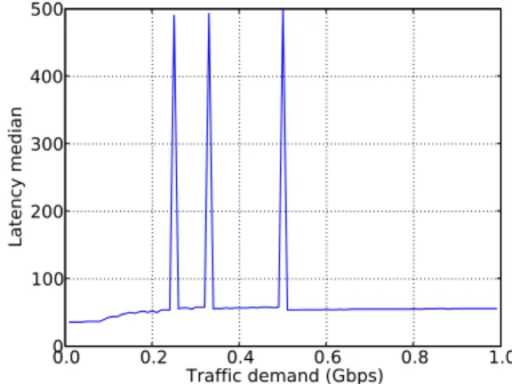
Figure 14: Latency vs demand, with uniform traffic.
by the kernel, and we record the latency of each re-ceived packet, as well as the number of drops. This test is useful mainly to quantify PC-induced latency variability. In the single-bottleneck case, two hosts send 0.7 Gbps of constant-rate traffic to a single switch output port, which connects through a second switch to a receiver. Concurrently with the packet generator traffic, the latency monitor sends tracer packets. In the double-bottleneck case, three hosts send 0.7 Gbps, again while tracers are sent.
Table 4 shows the latency distribution of tracer packets sent through the Quanta switch, for all three cases. With no background traffic, the baseline la-tency is 36 us. In the single-bottleneck case, the egress buffer fills immediately, and packets expe-rience 474 us of buffering delay. For the double-bottleneck case, most packets are delayed twice, to 914 us, while a smaller fraction take the single-bottleneck path. The HP switch (data not shown) follows the same pattern, with similar minimum la-tency and about 1500 us of buffer depth. All cases show low measurement variation.
4.2
Uniform Traffic, Varying Demand
In Figure 14, we see the latency totals for a uni-form traffic series where all traffic goes through the core to a different pod, and every hosts sends one flow. To allow the network to reach steady state, measurements start 100 ms after packets are sent,
0
100
overload (Mbps / Host)
200
300
400
500
0
5
10
15
20
25
30
35
40
Loss percentage (%)
margin:0.01Gbps
margin:0.05Gbps
margin:0.15Gbps
margin:0.2Gbps
margin:0.25Gbps
Figure 15: Drops vs overload with varying safety margins
and continue until the end of the test, 900 ms later. All tests use 512-byte packets; other packet sizes yield the same results. The graph covers packet generator traffic from idle to 1 Gbps, while tracer packets are sent along every flow path. If our solu-tion is feasible, that is, all flows on each link sum to less than its capacity, then we will see no dropped packets, with a consistently low latency.
Instead, we observe sharp spikes at 0.25 Gbps, 0.33 Gbps, and 0.5 Gbps. These spikes correspond to points where the available link bandwidth is ex-ceeded, even by a small amount. For example, when ElasticTree compresses four 0.25 Gbps flows along a single 1 Gbps link, Ethernet overheads (preamble, inter-frame spacing, and the CRC) cause the egress buffer to fill up. Packets either get dropped or sig-nificantly delayed.
This example motivates the need for a safety margin to account for processing overheads, traffic bursts, and sustained load increases. The issue is not just that drops occur, but also thatevery packet on an overloaded link experiences significant delay. Next, we attempt to gain insight into how to set the safety margin, or capacity reserve, such that perfor-mance stays high up to a known traffic overload.
4.3
Setting Safety Margins
Figures 15 and 16 show drops and latency as a function of traffic overload, for varying safety mar-gins. Safety margin is the amount of capacity re-served ateverylink by the optimizer; a higher safety margin provides performance insurance, by delaying the point at which drops start to occur, and aver-age latency starts to degrade. Traffic overload is the amount each host sends and receives beyond the original traffic matrix. The overload for a host is
0
100
overload (Mbps / Host)
200
300
400
500
0
100
200
300
400
500
600
700
800
900
Average Latency (usec)
margin:0.01Gbps
margin:0.05Gbps
margin:0.15Gbps
margin:0.2Gbps
margin:0.25Gbps
Figure 16: Latency vs overload with varying safety margins
10
210
310
4Total Hosts
10
-410
-310
-210
-110
010
110
210
3Computation time (s)
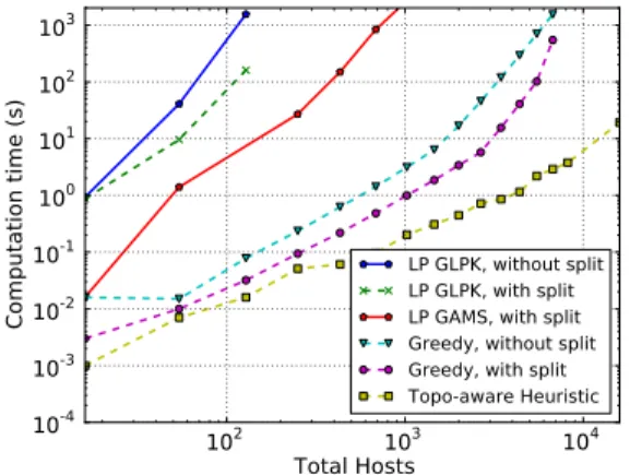
LP GLPK, without split LP GLPK, with split LP GAMS, with split Greedy, without split Greedy, with split Topo-aware HeuristicFigure 17: Computation time for different op-timizers as a function of network size
spread evenly across all flows sent by that host. For example, at zero overload, a solution with a safety margin of 100 Mbps will prevent more than 900 Mbps of combined flows from crossing each link. If a host sends 4 flows (as in these plots) at 100 Mbps overload, each flow is boosted by 25 Mbps. Each data point represents the average over 5 traffic ma-trices. In all matrices, each host sends to 4 randomly chosen hosts, with a total outgoing bandwidth se-lected uniformly between 0 and 0.5 Gbps. All tests complete in one second.
Drops Figure 15 shows no drops for small overloads (up to 100 Mbps), followed by a steadily increasing drop percentage as overload increases. Loss percentage levels off somewhat after 500 Mbps, as some flows cap out at 1 Gbps and generate no extra traffic. As expected, increasing the safety margin defers the point at which performance degrades.
LatencyIn Figure16, latency shows a trend sim-ilar to drops, except when overload increases to 200 Mbps, the performance effect is more pronounced. For the 250 Mbps margin line, a 200 Mbps over-load results in 1% drops, however latency increases by 10x due to the few congested links. Some margin lines cross at high overloads; this is not to say that a smaller margin is outperforming a larger one, since drops increase, and we ignore those in the latency calculation.
InterpretationGiven these plots, a network op-erator can choose the safety margin that best bal-ances the competing goals of performance and en-ergy efficiency. For example, a network operator might observe from past history that the traffic av-erage never varies by more than 100 Mbps in any 10 minute span. She considers an average latency under 100 us to be acceptable. Assuming that Elas-ticTree can transition to a new subset every 10 min-utes, the operator looks at 100 Mbps overload on each plot. She then finds the smallest safety margin with sufficient performance, which in this case is 150 Mbps. The operator can then have some assurance that if the traffic changes as expected, the network will meet her performance criteria, while consuming the minimum amount of power.
5.
PRACTICAL CONSIDERATIONS
Here, we address some of the practical aspects of deploying ElasticTree in a live data center environ-ment.
5.1
Comparing various optimizers
We first discuss the scalability of various optimiz-ers in ElasticTree, based on solution time vs network size, as shown in Figure17. This analysis provides a sense of the feasibility of their deployment in a real data center. The formal model produces solu-tions closest to optimal; however for larger topolo-gies (such as fat trees with k >= 14), the time to find the optimal solution becomes intractable. For example, finding a network subset with the formal model with flow splitting enabled on CPLEX on a single core, 2 Ghz machine, for a k = 16 fat tree, takes about an hour. The solution time growth of this carefully optimized model is about O(n3.5), where n is the number of hosts. We then ran the greedy-bin packer (written in unoptimized Python) on a single core of a 2.13 Ghz laptop with 3 GB of RAM. The no-split version scaled as aboutO(n2.5), while the with-split version scaled slightly better, as O(n2). The topology-aware heuristic fares much better, scaling as roughly O(n), as expected.
Sub-set computation for 10K hosts takes less than 10 seconds for a single-core, unoptimized, Python im-plementation – faster than the fastest switch boot time we observed (30 seconds for the Quanta switch). This result implies that the topology-aware heuris-tic approach is not fundamentally unscalable, espe-cially considering that the number of operations in-creases linearly with the number of hosts. We next describe in detail the topology-aware heuristic, and show how small modifications to its “starter subset” can yield high-quality, practical network solutions, in little time.
5.2
Topology-Aware Heuristic
We describe precisely how to calculate the subset of active network elements using only port counters.
Links. First, compute LEdgeup
p,e, the minimum
number of active links exiting edge switchein pod pto support up-traffic (edge→agg):
LEdgeup p,e=⌈(
X
a∈Ap
F(e→a))/r⌉
Ap is the set of aggregation switches in pod p,
F(e → a) is the traffic flow from edge switch e to aggregation switch a, and r is the link rate. The total up-traffic ofe, divided by the link rate, equals the minimum number of links from e required to satisfy the up-traffic bandwidth. Similarly, compute LEdgedown
p,e , the number of active links exiting edge
switch e in pod p to support down-traffic (agg → edge):
LEdgedownp,e =⌈(
X
a∈Ap
F(a→e))/r⌉
The maximum of these two values (plus 1, to en-sure a spanning tree at idle) givesLEdgep,e, the
min-imum number of links for edge switchein pod p: LEdgep,e= max{LEdgeupp,e, LEdgedownp,e ,1}
Now, compute the number of active links from each pod to the core. LAggup
p is the minimum
num-ber of links from pod p to the core to satisfy the up-traffic bandwidth (agg→core):
LAggupp =⌈(
X
c∈C,a∈Ap,a→c
F(a→c))/r⌉
Hence, we find the number of up-links,LAggdown p
used to support down-traffic (core→agg) in podp: LAggdownp =⌈(
X
c∈C,a∈Ap,c→a
F(c→a))/r⌉
The maximum of these two values (plus 1, to en-sure a spanning tree at idle) givesLAggp, the
mini-mum number of core links for podp: LAggp= max{LEdgeupp , LEdgedownp }
Switches. For both the aggregation and core lay-ers, the number of switches follows directly from the link calculations, as every active link must connect to an active switch. First, we computeN Aggup
p , the
minimum number of aggregation switches required to satisfy up-traffic (edge→agg) in podp:
N Aggup p = max
e∈Ep
{LEdgeup p,e}
Next, computeN Aggdown
p , the minimum number
of aggregation switches required to support down-traffic (core→agg) in podp:
N Aggdown
p =⌈(LAggdownp /(k/2)⌉
C is the set of core switches and k is the switch degree. The number of core links in the pod, divided by the number of links uplink in each aggregation switch, equals the minimum number of aggregation switches required to satisfy the bandwidth demands from all core switches. The maximum of these two values givesN Aggp, the minimum number of active
aggregation switches in the pod:
N Aggp= max{N Aggupp , N Aggpdown,1}
Finally, the traffic between the core and the most-active pod informs N Core, the number of core switches that must be active to satisfy the traffic demands:
N Core=⌈max
p∈P(LAgg up p )⌉
Robustness. The equations above assume that 100% utilized links are acceptable. We can change r, the link rate parameter, to set the desired aver-age link utilization. Reducing rreserves additional resources to absorb traffic overloads, plus helps to reduce queuing delay. Further, if hashing is used to balance flows across different links, reducingrhelps account for collisions.
To addk-redundancy to the starter subset for im-proved fault tolerance, add k aggregation switches to each pod and the core, plus activate the links on all added switches. Addingk-redundancy can be thought of as adding k parallel MSTs that overlap at the edge switches. These two approaches can be combined for better robustness.
5.3
Response Time
The ability of ElasticTree to respond to spikes in traffic depends on the time required to gather statis-tics, compute a solution, wait for switches to boot, enable links, and push down new routes. We mea-sured the time required to power on/off links and
switches in real hardware and find that the domi-nant time is waiting for the switch to boot up, which ranges from 30 seconds for the Quanta switch to about 3 minutes for the HP switch. Powering indi-vidual ports on and off takes about 1−3 seconds. Populating the entire flow table on a switch takes un-der 5 seconds, while reading all port counters takes less than 100 ms for both. Switch models in the fu-ture may support feafu-tures such as going into various sleep modes; the time taken to wake up from sleep modes will be significantly faster than booting up. ElasticTree can then choose which switches to power off versus which ones to put to sleep.
Further, the ability to predict traffic patterns for the next few hours for traces that exhibit regular behavior will allow network operators to plan ahead and get the required capacity (plus some safety mar-gin) ready in time for the next traffic spike. Al-ternately, a control loop strategy to address perfor-mance effects from burstiness would be to dynami-cally increase the safety margin whenever a thresh-old set by a service-level agreement policy were ex-ceeded, such as a percentage of packet drops.
5.4
Traffic Prediction
In all of our experiments, we input the entire traf-fic matrix to the optimizer, and thus assume that we have complete prior knowledge of incoming traf-fic. In a real deployment of ElasticTree, such an assumption is unrealistic. One possible workaround is to predict the incoming traffic matrix based on historical traffic, in order to plan ahead for expected traffic spikes or long-term changes. While predic-tion techniques are highly sensitive to workloads, they are more effective for traffic that exhibit regular patterns, such as our production data center traces (§3.1.4). We experiment with a simple auto regres-sive AR(1) prediction model in order to predict fic to and from each of the 292 servers. We use traf-fic traces from the first day to train the model, then use this model to predict traffic for the entire 5 day period. Using the traffic prediction, the greedy bin-packer can determine an active topology subset as well as flow routes.
While detailed traffic prediction and analysis are beyond the scope of this paper, our initial exper-imental results are encouraging. They imply that even simple prediction models can be used for data center traffic that exhibits periodic (and thus pre-dictable) behavior.
5.5
Fault Tolerance
ElasticTree modules can be placed in ways that mitigate fault tolerance worries. In our testbed, the
routing and optimizer modules run on a single host PC. This arrangement ties the fate of the whole sys-tem to that of each module; an optimizer crash is capable of bringing down the system.
Fortunately, the topology-aware heuristic – the optimizer most likely to be deployed – operates inde-pendently of routing. The simple solution is to move the optimizer to a separate host to prevent slow computation or crashes from affecting routing. Our OpenFlow switches support a passive listening port, to which the read-only optimizer can connect to grab port statistics. After computing the switch/link sub-set, the optimizer must send this subset to the rout-ing controller, which can apply it to the network. If the optimizer doesn’t check in within a fixed pe-riod of time, the controller should bring all switches up. The reliability of ElasticTree should be no worse than the optimizer-less original; the failure condition brings back the original network power, plus a time period with reduced network capacity.
For optimizers tied to routing, such as the for-mal model and greedy bin-packer, known techniques can provide controller-level fault tolerance. In active standby, the primary controller performs all required tasks, while the redundant controllers stay idle. On failing to receive a periodic heartbeat from the mary, a redundant controller becomes to the new pri-mary. This technique has been demonstrated with NOX, so we expect it to work with our system. In the more complicated full replication case, multiple controllers are simultaneously active, and state (for routing and optimization) is held consistent between them. For ElasticTree, the optimization calculations would be spread among the controllers, and each controller would be responsible for power control for a section of the network. For a more detailed discus-sion of these issues, see §3.5 “Replicating the Con-troller: Fault-Tolerance and Scalability” in [5].
6.
RELATED WORK
This paper tries to extend the idea of power pro-portionality into the network domain, as first de-scribed by Barrosoet al. [4]. Guptaet al. [17] were amongst the earliest researchers to advocate con-serving energy in networks. They suggested putting network components to sleep in order to save en-ergy and explored the feasibility in a LAN setting in a later paper [18]. Several others have proposed techniques such as putting idle components in a switch (or router) to sleep [18] as well as adapting the link rate [14], including the IEEE 802.3az Task Force [19].
Chabareket al.[6] use mixed integer programming to optimize router power in a wide area network, by
choosing the chassis and linecard configuration to best meet the expected demand. In contrast, our formulation optimizes a data center local area net-work, finds the power-optimal network subset and routing to use, and includes an evaluation of our prototype. Further, we detail the tradeoffs associ-ated with our approach, including impact on packet latency and drops.
Nedevschi et al. [26] propose shaping the traffic into small bursts at edge routers to facilitate putting routers to sleep. Their research is complementary to ours. Further, their work addresses edge routers in the Internet while our algorithms are for data cen-ters. In a recent work, Ananthanarayanan [3] et al. motivate via simulation two schemes - a lower power mode for ports and time window prediction techniques that vendors can implemented in future switches. While these and other improvements can be made in future switch designs to make them more energy efficient, most energy (70-80% of their total power) is consumed by switches in their idle state. A more effective way of saving power is using a traf-fic routing approach such as ours to maximize idle switches and power them off. Another recent pa-per [25]et al. discusses the benefits and deployment models of a network proxy that would allow end-hosts to sleep while the proxy keeps the network connection alive.
Other complementary research in data center net-works has focused on scalability [24][10], switching layers that can incorporate different policies [20], or architectures with programmable switches [11].
7.
DISCUSSION
The idea of disabling critical network infrastruc-ture in data centers has been considered taboo. Any dynamic energy management system that attempts to achieve energy proportionality by powering off a subset of idle components must demonstrate that the active components can still meet the current of-fered load, as well as changing load in the immedi-ate future. The power savings must be worthwhile, performance effects must be minimal, and fault tol-erance must not be sacrificed. The system must pro-duce a feasible set of network subsets that can route to all hosts, and be able to scale to a data center with tens of thousands of servers.
To this end, we have built ElasticTree, which through data-center-wide traffic management and control, introduces energy proportionality in today’s non-energy proportional networks. Our initial re-sults (covering analysis, simulation, and hardware prototypes) demonstrate the tradeoffs between
per-formance, robustness, and energy; the safety mar-gin parameter provides network administrators with control over these tradeoffs. ElasticTree’s ability to respond to sudden increases in traffic is currently limited by the switch boot delay, but this limita-tion can be addressed, relatively simply, by adding a sleep mode to switches.
ElasticTree opens up many questions. For exam-ple, how will TCP-based application traffic interact with ElasticTree? TCP maintains link utilization in sawtooth mode; a network with primarily TCP flows might yield measured traffic that stays below the threshold for a small safety margin, causing Elas-ticTree to never increase capacity. Another ques-tion is the effect of increasing network size: a larger network probably means more, smaller flows, which pack more densely, and reduce the chance of queuing delays and drops. We would also like to explore the general applicability of the heuristic to other topolo-gies, such as hypercubes and butterflies.
Unlike choosing between cost, speed, and relia-bility when purchasing a car, with ElasticTree one doesn’t have to pick just two when offered perfor-mance, robustness, and energy efficiency. During periods of low to mid utilization, and for a variety of communication patterns (as is often observed in data centers), ElasticTree can maintain the robust-ness and performance, while lowering the energy bill.
8.
ACKNOWLEDGMENTS
The authors want to thank their shepherd, Ant Rowstron, for his advice and guidance in produc-ing the final version of this paper, as well as the anonymous reviewers for their feedback and sugges-tions. Xiaoyun Zhu (VMware) and Ram Swami-nathan (HP Labs) contributed to the problem for-mulation; Parthasarathy Ranganathan (HP Labs) helped with the initial ideas in this paper. Thanks for OpenFlow switches goes to Jean Tourrilhes and Praveen Yalagandula at HP Labs, plus the NEC IP8800 team. Greg Chesson provided the Google traces.
9.
REFERENCES
[1] M. Al-Fares, A. Loukissas, and A. Vahdat. A Scalable,
Commodity Data Center Network Architecture. InACM
SIGCOMM, pages 63–74, 2008.
[2] M. Al-Fares, S. Radhakrishnan, B. Raghavan, N. Huang, and A. Vahdat. Hedera: Dynamic Flow Scheduling for Data
Center Networks. InUSENIX NSDI, April 2010.
[3] G. Ananthanarayanan and R. Katz. Greening the Switch. InProceedings of HotPower, December 2008.
[4] L. A. Barroso and U. H¨olzle. The Case for
Energy-Proportional Computing.Computer, 40(12):33–37,
2007.
[5] M. Casado, M. Freedman, J. Pettit, J. Luo, N. McKeown, and S. Shenker. Ethane: Taking control of the enterprise. InProceedings of the 2007 Conference on Applications,
Technologies, Architectures, and Protocols for Computer Communications, page 12. ACM, 2007.
[6] J. Chabarek, J. Sommers, P. Barford, C. Estan, D. Tsiang, and S. Wright. Power Awareness in Network Design and
Routing. InIEEE INFOCOM, April 2008.
[7] U.S. Environmental Protection Agency’s Data Center
Report to Congress.http://tinyurl.com/2jz3ft.
[8] S. Even, A. Itai, and A. Shamir. On the Complexity of
Time Table and Multi-Commodity Flow Problems. In16th
Annual Symposium on Foundations of Computer Science, pages 184–193, October 1975.
[9] A. Greenberg, J. Hamilton, D. Maltz, and P. Patel. The Cost of a Cloud: Research Problems in Data Center
Networks. InACM SIGCOMM CCR, January 2009.
[10] A. Greenberg, N. Jain, S. Kandula, C. Kim, P. Lahiri, D. Maltz, P. Patel, and S. Sengupta. VL2: A Scalable and
Flexible Data Center Network. InACM SIGCOMM,
August 2009.
[11] A. Greenberg, P. Lahiri, D. A. Maltz, P. Patel, and S. Sengupta. Towards a Next Generation Data Center
Architecture: Scalability and Commoditization. InACM
PRESTO, pages 57–62, 2008.
[12] D. Grunwald, P. Levis, K. Farkas, C. M. III, and M. Neufeld. Policies for Dynamic Clock Scheduling. In
OSDI, 2000.
[13] N. Gude, T. Koponen, J. Pettit, B. Pfaff, M. Casado, and N. McKeown. NOX: Towards an Operating System for
Networks. InACM SIGCOMM CCR, July 2008.
[14] C. Gunaratne, K. Christensen, B. Nordman, and S. Suen. Reducing the Energy Consumption of Ethernet with
Adaptive Link Rate (ALR).IEEE Transactions on
Computers, 57:448–461, April 2008.
[15] C. Guo, G. Lu, D. Li, H. Wu, X. Zhang, Y. Shi, C. Tian, Y. Zhang, and S. Lu. BCube: A High Performance, Server-centric Network Architecture for Modular Data
Centers. InACM SIGCOMM, August 2009.
[16] C. Guo, H. Wu, K. Tan, L. Shi, Y. Zhang, and S. Lu. DCell: A Scalable and Fault-Tolerant Network Structure
for Data Centers. InACM SIGCOMM, pages 75–86, 2008.
[17] M. Gupta and S. Singh. Greening of the internet. InACM
SIGCOMM, pages 19–26, 2003.
[18] M. Gupta and S. Singh. Using Low-Power Modes for
Energy Conservation in Ethernet LANs. InIEEE
INFOCOM, May 2007.
[19] IEEE 802.3az.ieee802.org/3/az/public/index.html.
[20] D. A. Joseph, A. Tavakoli, and I. Stoica. A Policy-aware
Switching Layer for Data Centers.SIGCOMM Comput.
Commun. Rev., 38(4):51–62, 2008.
[21] S. Kandula, D. Katabi, S. Sinha, and A. Berger. Dynamic
Load Balancing Without Packet Reordering.SIGCOMM
Comput. Commun. Rev., 37(2):51–62, 2007. [22] P. Mahadevan, P. Sharma, S. Banerjee, and
P. Ranganathan. A Power Benchmarking Framework for
Network Devices. InProceedings of IFIP Networking, May
2009.
[23] J. Mudigonda, P. Yalagandula, M. Al-Fares, and J. C. Mogul. SPAIN: COTS Data-Center Ethernet for
Multipathing over Arbitrary Topologies. InUSENIX
NSDI, April 2010.
[24] R. Mysore, A. Pamboris, N. Farrington, N. Huang, P. Miri, S. Radhakrishnan, V. Subramanya, and A. Vahdat. PortLand: A Scalable Fault-Tolerant Layer 2 Data Center
Network Fabric. InACM SIGCOMM, August 2009.
[25] S. Nedevschi, J. Chandrashenkar, B. Nordman,
S. Ratnasamy, and N. Taft. Skilled in the Art of Being Idle: Reducing Energy Waste in Networked Systems. In Proceedings Of NSDI, April 2009.
[26] S. Nedevschi, L. Popa, G. Iannaccone, S. Ratnasamy, and D. Wetherall. Reducing Network Energy Consumption via
Sleeping and Rate-Adaptation. InProceedings of the 5th
USENIX NSDI, pages 323–336, 2008.
[27] Cisco IOS NetFlow.http://www.cisco.com/web/go/netflow.
[28] NetFPGA Packet Generator.http://tinyurl.com/ygcupdc.
[29] The OpenFlow Switch.http://www.openflowswitch.org.
[30] C. Patel, C. Bash, R. Sharma, M. Beitelmam, and R. Friedrich. Smart Cooling of data Centers. In Proceedings of InterPack, July 2003.
APPENDIX
A.
POWER OPTIMIZATION PROBLEM
Our model is a multi-commodity flow formulation, augmented with binary variables for the power state of links and switches. It minimizes the total network power by solving a mixed-integer linear program.
A.1
Multi-Commodity Network Flow
Flow network G(V, E), has edges (u, v) ∈ E with capacity c(u, v). There are k commodities K1, K2, . . . , Kk, defined byKi = (si, ti, di), where,
for commodityi,si is the source,tiis the sink, and
di is the demand. The flow of commodity i along
edge (u, v) isfi(u, v). Find a flow assignment which
satisfies the following three constraints [8]:
Capacity constraints: The total flow along each link must not exceed the edge capacity.
∀(u, v)∈V,
k
X
i=1
fi(u, v)≤c(u, v)
Flow conservation: Commodities are neither created nor destroyed at intermediate nodes.
∀i,X
w∈V
fi(u, w) = 0,whenu6=siand u6=ti
Demand satisfaction: Each source and sink sends or receives an amount equal to its demand.
∀i,X w∈V fi(si, w) = X w∈V fi(w, ti) =di
A.2
Power Minimization Constraints
Our formulation uses the following notation: S Set of all switches
Vu Set of nodes connected to a switchu
a(u, v) Power cost for link (u, v) b(u) Power cost for switchu
Xu,v Binary decision variable indicating
whether link (u, v) is powered ON Yu Binary decision variable indicating
whether switchuis powered ON Ei Set of all unique edges used by flowi
ri(u, v) Binary decision variable indicating
whether commodityiuses link (u, v) The objective function, which minimizes the total network power consumption, can be represented as:
Minimize P(u,v)∈EXu,v×a(u, v)+Pu∈V Yu×b(u)
The following additional constraints create a de-pendency between the flow routing and power states:
Deactivated links have no traffic: Flow is re-stricted to only those links (and consequently the switches) that are powered on. Thus, for all links (u, v) used by commodity i, fi(u, v) = 0,
when Xu,v = 0. Since the flow variable f is
positive in our formulation, the linearized con-straint is:
∀i,∀(u, v)∈E,
k
X
i=1
fi(u, v)≤c(u, v)×Xu,v
The optimization objective inherently enforces the converse, which states that links with no traffic can be turned off.
Link power is bidirectional: Both “halves” of an Ethernet link must be powered on if traffic is flowing in either direction:
∀(u, v)∈E, Xu,v=Xv,u
Correlate link and switch decision variable:
When a switch u is powered off, all links connected to this switch are also powered off:
∀u∈V,∀w∈Vv, Xu,w =Xw,u≤Yu
Similarly, when all links connecting to a switch are off, the switch can be powered off. The lin-earized constraint is:
∀u∈V, Yu≤
X
w∈Vu
Xw,u
A.3
Flow Split Constraints
Splitting flows is typically undesirable due to TCP packet reordering effects [21]. We can prevent flow splitting in the above formulation by adopting the following constraint, which ensures that the traffic on link (u, v) of commodityi is equal to either the full demand or zero:
∀i,∀(u, v)∈E, fi(u, v) =di×ri(u, v)
The regularity of the fat tree, combined with re-stricted tree routing, helps to reduce the number of flow split binary variables. For example, each inter-pod flow must go from the aggregation layer to the core, with exactly (k/2)2 path choices. Rather than consider binary variabler for all edges along every possible path, we only consider the set of “unique edges”, those at the highest layer traversed. In the inter-pod case, this is the set of aggregation to edge links. We precompute the set of unique edges Ei
usable by commodityi, instead of using all edges in E. Note that the flow conservation equations will ensure that a connected set of unique edges are tra-versed for each flow.