Articles
1
Pattern matching trading system based on the
2
dynamic time warping algorithm
3
Sang Hyuk Kim 1, Hee Soo Lee 2, Hanjun Ko 3, Seung Hwan Jeong 4, Hyun Woo Byun 5,
4
and Kyong Joo Oh 6,*
5
1 Department of Industrial Engineering, Yonsei University; [email protected]
6
2 Department of Business Administration, Sejong University; [email protected]
7
3 Department of Industrial Engineering, Yonsei University; [email protected]
8
4 Department of Industrial Engineering, Yonsei University; [email protected]
9
5 Department of Industrial Engineering, Yonsei University; [email protected]
10
6 Department of Industrial Engineering, Yonsei University
11
* Correspondence: [email protected]; Tel.: +82-2-2123-5720
12
13
Abstract: The futures market plays a significant role in hedging and speculating by investors.
14
Although various models and instruments are developed for real-time trading, it is difficult to
15
realize profit by processing and trading a vast amount of real-time data. This study proposes a
16
real-time index futures trading strategy that uses the pattern of KOSPI 200 index futures time series
17
data. We construct a pattern matching trading system (PMTS) based on a dynamic time warping
18
algorithm that recognizes patterns of market data movement in the morning and determines the
19
afternoon's clearing strategy. We adopt 13 and 27 representative patterns and conduct simulations
20
with various ranges of parameters to find optimal ones. Our experimental results show that the
21
PMTS provides stable and effective trading strategies with relatively low trading frequencies.
22
Investor communities that have sustained financial markets are able to make more efficient
23
investments by using the PMTS. In this sense, the system developed in this paper is a sustainable
24
investment technique and helps financial markets achieve efficient sustainability.
25
Keywords: Dynamic time warping; Pattern matching trading system; Time series data; Sliding
26
window
27
28
1. Introduction
29
The global financial crisis of 2007- 2008 (GFC) was caused by many factors, but one of the main
30
causes was the excessive expansion of financial assets including derivatives (F. R. Birau, 2012; J.
31
Carmassi, D. Gros, S. Micossi, 2009; J. Crotty, 2009). The world's leading financial markets include
32
major equity index futures such as the S&P 500, NASDAQ 100, DJIA, FTSE Russel 100, Nikkei 225
33
and KOSPI 200. Among them, the KOSPI 200 futures and options markets have been the largest
34
trading market since prior to the GFC until the mid-2010s (Ghysels and Seon, 2005). As a single time
35
series data, the index futures, which generate a large amount of data as a result of large-scale
36
transactions, have been widely used for statistical analysis (Kwon, Lee, 2014, T.T.H. Phan, E. P.
37
Caillault, A. Lefebvre, A. Bigand., 2017). In recent years, data mining and machine learning
38
techniques are utilized to investigate the futures market.
39
Time series data is a collection of observational data that is generated chronologically from
40
most scientific and business domains (E. J. Keogh, M. J. Pazzani, 1999). Many researchers in various
41
fields have used time series data for their research (G. Das, D. Gunopulos, H. Mannila, 1997; R.
42
Agrawal, C. Faloutsos, A. N. Swami, 1993). Time series data in financial markets have unique
43
characteristics compared to that in other fields such as electrocardiograms (T.C. Fu, F.L. Chung, R.
44
Luk, C.M. Ng, 2006). In stock price time series data, investors in equity markets show various
45
patterns of investment. They can be categorized as investors who adopt fundamental analysis and
46
technical analysis (Bagheri, Peyhani, and Akbari, 2014). Fundamental analysts make investment
47
decisions using global economic, industry and business indicators. On the other hand, assuming that
48
the past behavior of a stock price affects the future price, technical analysts make investment
49
decisions based on historical prices or patterns of price movement using complex indicators.
50
Accordingly, technical analysts use pattern analysis methods to analyze stock price charts for
51
trading decisions (Deboeck, 1994). Many studies on technical analysis for pattern matching have
52
been carried out (Lo et al., 2000; Leigh et al., 2002, 2004). This pattern analysis is a method of
53
predicting the stock price by examining specific patterns observed in the past stock price chart and
54
confirming the existence of similar patterns in the current stock price (T.L. Chen, F.Y. Chen, 2016).
55
An algorithm for efficient pattern recognition of the time series data is needed to build a trading
56
system based on pattern recognition. The Euclidean distance method or artificial intelligence
57
method has been used to find a similar pattern for stock prices (Kim et al, 2002; Chung et al, 2004;
58
Dong, Zhou, 2002). Hu et al., (2015) proposed a model which is an investment strategy using a short-
59
and long-term evolutionary trend algorithm. De Oliveira, Nobre, and Zarate, (2013) also proposed a
60
model for predicting stock prices in the Brazilian market which combines fundamental and technical
61
analysis using artificial neural networks. The system development includes forecasting the FX
62
market financial time series, which combines an adaptive network-based fuzzy inference system and
63
quantum behavioral particle gain optimization, and forecasting market trends using chart patterns
64
(Bagheri et al., 2014). Patel et al. (2015) also proposed a model to predict trends in financial markets
65
by comparing four predictive models such as artificial neural networks, support vector machines,
66
random forests, and naïve-Bayes. There are also studies showing the efficiency of dynamic time
67
warping algorithms for the problem of retrieving multiattribute time sequences similar to financial
68
time series data (T. Kahveci, A. Singh, and A. Gurel, 2002). The proposed method based on the
69
dynamic time warping algorithm predefines the pattern used as a template for pattern matching
70
(Berndt and Clifford, 1994). These studies have focused on optimization and efficiency in pattern
71
recognition. However, there is a limit to a study on system trading at the optimal trading time point
72
by checking the similarity of existing patterns in the futures market. This trading strategy requires
73
efficient pattern recognition algorithms such as dynamic time warping (P. Senin, 2008). Among
74
them, only a few studies use the dynamic time warping algorithm for futures trading (Lee, S.J., Ahn,
75
J.J., Oh, K.J., Kim, T.Y., 2010, 2012).
76
The purpose of this research is to construct a pattern matching trading system (PMTS) that
77
extracts efficiently the optimized pattern of the proposed representative pattern in time series data
78
and conducts trading to find the optimal trading exit point. For this goal, we propose an algorithm
79
trading system that matches the time series pattern of the index futures data with the representative
80
pattern using the naïve dynamic time warping (DTW) algorithm. As the experiment progresses, we
81
consider various situations in futures contracts such as when margin calls are made, the liquidity
82
and volatility increases, the trend changes for trades that enter into the calculation of the intraday
83
trade, and trades exit right before the closing of the market, to find the optimal trading exit point.
84
Our experimental results show stable and effective trading entry and exit strategies with relatively
85
low trading frequencies. Investor communities that have sustained financial markets are able to
86
make more efficient investments by using the PMTS. In this sense, the system developed in this
87
paper is a sustainable investment technique and helps financial markets achieve efficient
88
sustainability.
89
The rest of this paper is organized as follows. Section 2 introduces the concept of futures
90
markets, the concept of dynamic time warping algorithms and the sliding window method. In
91
Section 3, the topics include the standardization of extracted raw daily index futures data, the
92
dynamic trading pattern together with the dynamic time warping analysis for real-time pattern
93
recognition, and the proposed trading entry and exit simulation. Section 3.4 describes the procedure
94
of the experiments performed and discusses the experimental results. Section 4 interprets the results
95
and suggests the direction of future research.
96
2. Materials and Methods
98
2.1. Futures Market
99
The futures market is a market for futures trading, which is one of many derivatives. The value
100
of derivatives relies on other assets called underlying assets such as commodities, stocks, bonds,
101
indices, and interest rates. In other words, it changes when the value of the underlying assets
102
changes. Prior to the establishment of futures markets, forward contracts have been traded to avoid
103
the risk related to the value of the underlying asset. When one does not need to have the underlying
104
asset at the present time but needs it in the future, he or she can make a forward contract with a
105
counter party that presents the underlying asset’s delivery price and date. Due to the credit risk
106
inherent in the forward contract, futures markets have been established by standardizing
107
transactions and eliminating the credit risk.
108
The futures market was originally designed to help market participants avoid exposure to the
109
risk of price fluctuations. In recent years, the role of risk hedging by futures contracts has become
110
more prominent. For instance, although KOSPI 200 index futures are recognized as a high-return
111
investment, the primary purpose of investing in the stock index futures is to avoid the risk related to
112
stock prices. The stock index futures’ underlying asset is a stock price index which is an intangible
113
product, and hence it cannot be acquired or delivered to the counter party of the contract. Investors
114
in index futures have a long position when the bull market is predicted and have a short position
115
when the bear market is predicted in the future. Accordingly, investors in index futures can realize
116
profits in both bull and bear markets if they make a correct prediction. In other words, they should
117
predict the direction of stock price fluctuations accurately. They are not able to realize efficient yields
118
by responding promptly with intuitive and qualitative investment decisions based on past trading
119
experience. Indeed, quantitative and systematized trading strategies which use existing futures
120
investment strategies and past time series data are required for realizing efficient yields. It is
121
essential to develop a quantitative method to determine the most useful trading positions and
122
timing of index futures to realize high yields.
123
An investor in a futures market is classified as a hedger who avoids risk and a speculator who
124
seeks profit (Chang, 1985; Hartzmark, 1987, 1991; Leuthold et al, 1994; Wang, 2001). The hedger
125
takes the position to hedge the stock price risk and rollover the position until the settlement date,
126
whereas a speculator tends to clear his or her position whenever he or she can make profits. The
127
futures market operates a margin system to avoid the credit risk due to the leverage effect on
128
underlying assets. It includes the initial margin, maintenance margin, and additional margin. The
129
initial margin is at least 15% of the contract value and must be paid to enter a new futures contract.
130
The maintenance margin is at least 10% of the contract value and must be maintained for holding a
131
futures contract. Additional margin should be paid if the margin level is lower than the maintenance
132
margin as the futures price fluctuates. The additional margin payment is notified by brokerage
133
firms, which is called a margin call. If the margin call is triggered and the additional margin is not
134
paid, the exchange arbitrarily clears the outstanding position by making a reverse trading.
135
2.2. Dynamic Time Warping
136
The dynamic time warping (DTW) algorithm is known as an efficient method to measure the
137
similarity between two sequences of time series data. Intuitively, the sequences are warped in a
138
nonlinear fashion to match each other. The DTW minimizes distortion effects due to time-dependent
139
movement by using an elastic transformation of time series data to recognize the similar phases
140
between different patterns along time. Even if there is a deformation relationship between two
141
different sequences of time series data, the DTW determines the most similarities between them
142
(Keogh and Pazzani, 1999). Since the DTW was introduced in the 1960s (Bellman and Kalaba, 1959),
143
the algorithm has been applied to spoken word recognition (Sakoe and Chiba, 1978, Myers et al.,
144
1980), gesture recognition (Kuzmanic and Zanchi, 2007), behavioral perception (Corradini, 2001),
145
data mining, and time series clustering (Kahveci and Singh, 2001, Bahlmann and Burkhardt, 2004;
146
148
149
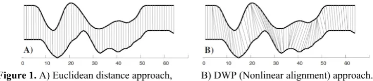
Figure 1. A) Euclidean distance approach, B) DWP (Nonlinear alignment) approach.
150
151
The objective of DTW is to compare two time series 𝑋 = (𝓍 , 𝓍 , ⋯ , 𝓍 ), 𝑁 ∈ ℕ and 𝑌 =
152
(𝓎 , 𝓎 , ⋯ , 𝓎 ), 𝑀 ∈ ℕ and calculate the minimum cumulative distance between them (Muller, M.,
153
2007). Various modifications of the algorithm have been proposed to speed up DTW computations
154
such as multiscaling (Muller et al, 2006; Salvador and Chan., 2007). It is more efficient to use the local
155
distance measurement function when the value must be obtained in a specific space rather than
156
comparing two different sequence sets. The concept of the cost function or the distance
157
minimization, which is the core of DTW, is applied to a dynamic programming algorithm to produce
158
a small value when two sequences are similar and a large value when two sequences are not similar.
159
The algorithm provides a way to optimize the alignment and to minimize cost functions or the
160
distance.
161
The DTW algorithm creates a distance matrix 𝐶 ∈ ℝ × ∶ 𝑐, =∥ 𝓍 − 𝓎 ∥, 𝑖 ∈ [1: 𝑁], 𝑗 ∈ [1: 𝑀]
162
that represents all pairwise distances. It is called the local cost matrix for the alignment of two
163
sequences X and Y. After generating this matrix, the algorithm uses a warping function that defines
164
the similarity between 𝓍 ∈ 𝑋 and 𝓎 ∈ 𝑌, which follows the boundary condition of assigning the
165
first and last elements of X and Y, and finds the optimal alignment path to pass through. This
166
optimal alignment path is a continuous point of 𝑃 = (𝓅 , 𝓅 , ⋯ , 𝓅 ) with 𝓅 = (𝓅 , 𝓅 ) ∈ [1: 𝑁] ×
167
[1: 𝑀] for 𝑙 ∈ [1: 𝐾] that satisfies all three criteria of the boundary condition, the monotonicity
168
condition, and the step size condition. The boundary condition is the first and last values of
169
sequences in the optimal alignment path. The monotonicity condition is sequence of points on the
170
path placed in chronological order. The step size condition limits the long jumping warping path in
171
time. It is generally recommended to use the formulated basic step size condition as 𝓅 − 𝓅 ∈
172
{(1,1), (1,0), (0,1)}. The cost function used to calculate the local cost matrix of all the bidirectional
173
distances is:
174
𝑐 (𝑋, 𝑌) = 𝑐 𝓍 , 𝓎 (1)
The aligned warping path with the least cost is called the 𝑃∗ optimal warping path. By
175
definition, the optimal path increases exponentially as the length of X and Y increases linearly, so all
176
possible warping paths between X and Y, which consume a large amount of computation, must be
177
tested. This problem can be solved by O(MN) based on dynamic programming, the core of DTW.
178
The DTW distance between X and Y, DTW(X, Y), is then defined as the total cost of p∗ as follows:
179
𝐷𝑇𝑊(𝑋, 𝑌) = 𝑐 ∗(𝑋, 𝑌) = 𝑚𝑖𝑛 {𝑐 (𝑋, 𝑌), 𝑝 ∈ 𝑃 × }, (2)
where 𝑃 × is the set of all possible warping paths.
180
2.3. Pattern Matching Trading System
181
This section describes the structure and characteristics of the pattern matching trading system
182
(PMTS) used in experiments for index futures trading. The experiments determine the entry and exit
183
of trading by matching the daily index futures time series data with fixed patterns using the DTW
184
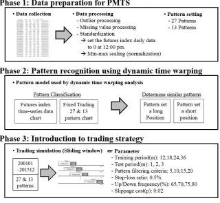
algorithm. Figure 2 shows an experimental procedure diagram of the pattern matching trading
185
system. The first phase of the procedure is to collect the daily index futures data and to preprocess
186
them for outlier processing, missing value processing, and standardization of the data from
187
KOSCOM’s Check Expert system. In the second phase, the fixed time series patterns and the
188
by the dynamic time warping algorithm. The third phase is to improve the performance with
190
training data for trading entry and exit simulations with various parameters and perform the
191
verification with testing data.
192
193
Figure 2. Process of PMTS.
194
195
Phase 1: Data preparation for the pattern matching trading system
196
To conduct this experiment, 137,242 KOSPI 200 index futures data were collected every at 10
197
minute intervals from 20010102 to 20151230. The collected index futures time series data are
198
preprocessed by outlier processing and missing value processing. All extracted daily index futures
199
data are standardized by setting the index futures data to 0 at 12:00 pm and scaling with the
200
min-max method. The scaled data is obtained by the following equation:
201
𝑓(𝑑) = ( ) ∈ ( )
∈ ( ) ∈ ( ), (3)
where 𝑓(𝑑), ∀𝑑 ∈ 𝐷𝑎𝑖𝑙𝑦 𝑓𝑢𝑡𝑢𝑟𝑒𝑠 𝑑𝑎𝑡𝑎 𝑠𝑒𝑡 (dfid) is the daily index futures data.
202
The processed data is divided into two groups: the pattern recognition group that consists of
203
data from 9:00 am to 12:00 pm and the trading group that consists of data after 12:00 pm. If there is
204
no data at 9:00 am due to a delayed market opening caused by a market action or regulation, the
205
missing data is filled with the closing price of the previous date.
206
207
Phase 2: Pattern recognition and determination of the trading position
208
We construct two sets of fixed patterns using two different time divisions. The time from 9:00
209
am to 12:00 pm is divided into three time zones (from 9 am to 10 am, from 10 am to 11 am, and from
210
11 am to 12 pm) and a total of 27 fixed time series patterns is set up consisting of all possible
211
combinations of three steps (upward, stable, and downward) in each time zone. The 27 fixed
212
patterns can be described by 9 representative roughness patterns as a result of eliminating the
213
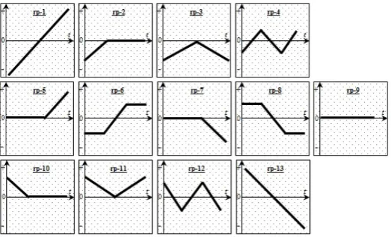
similarity in terms of macroscopic viewpoints and endpoints. In addition, the time from 9:00 am to
214
12:00 pm is divided into two time zones (or the first half from 9 am to 10:30 am and the second half
215
from 10:30 am to 12:00 pm) to set up 9 representative patterns consisting of three steps, and then 4
216
industry recommendation patterns are added to have 13 representative patterns. The figure below
217
219
220
Figure 3. Structures of the initial 27 patterns (ip# as initial pattern).
221
222
223
Figure 4. Structures of the representative 13 patterns (rp-# as representative pattern).
224
225
The daily market data between 9:00 am and 12:00 pm from 20010102 to 20151230 are assigned to
226
one of the fixed patterns that is the most similar to the market data by using the dynamic time
227
warping method, and then the frequency of each selected pattern is counted. At this step, the fixed
228
patterns with a higher frequency than the filtering criteria are selected. For each selected pattern of
229
the daily market data, the price at 12:00 pm and 3:00 pm on a day included in training period is
230
compared. Then, “up” is assigned to the pattern if the price at 3:00 pm is higher than that at 12:00
231
pm, and “down” is assigned to the pattern if the price at 3:00 pm is lower than that at 12:00 pm. The
232
ratio of “up” to “down” for each pattern is calculated and used to determine the trading position in
233
the testing period. Once a pattern from 9:00 am to 12:00 pm is selected for market data on one day
234
that is included in a testing period, the investment strategy at 12:00 pm on that day is determined as
235
follows:
236
237
- Enter a long position at 12:00 pm and clear the position by taking a short position at 3:00 pm
238
if the ratio of “up” to “down” for the selected pattern is higher than 1.
239
- Enter a short position at 12:00 pm and clear the position by taking a long position at 3:00 pm
240
if the ratio of “up” to “down” for the selected pattern is lower than 1.
241
242
The margin of the futures trading is settled at 12:00 pm when the volatility and liquidity
243
increase. Therefore, it is a critical time to enter a position. For intraday trades, the clearing time can
244
be used at various points in time and is not limited at 3:00 pm.
245
246
Phase 3: PMTS simulation
247
In the last phase, we performed PMTS simulation by applying trading rule created in Phase 2.
248
250
Figure 5. Workflow of the PMTS.
251
252
As shown in this figure, we first set the sample period using a sliding window method and
253
divide each window into training and testing periods. Then, using the DTW algorithm with various
254
ranges of parameters, we conduct pattern matching to daily index futures data and determine the
255
entry and exit position for the testing period. This process is repeated for all windows for the
256
selected parameters. As a last step, we analyze the trading profit and determine the optimal
257
parameters for PMTS. Figure 6 shows the structure of the sliding windows.
258
259
260
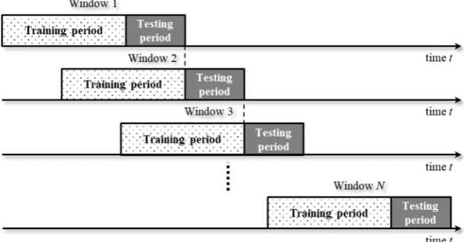
Figure 6. Structures of the sliding windows.
261
262
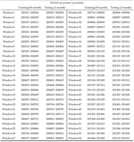
The sliding window method has been used for simulation of time series data (Hwarng, 2001;
263
Jang et al., 1993; Ahn et al., 2012; Chou and Ngo, 2016). Table 1 shows a set of 54 windows with an 18
264
month training period and a 3 month testing period. For example, Window1 is composed of the 18
265
month training period of 2001.01 - 2002.06 and the 3 month testing period of 2002.07 - 2002.09.
266
Sliding 3 months from Window1, Window2 is set with a training period of 2001.04 - 2002.09 and a
267
testing period of 2002.10 - 2002.12. The sliding is continued until the entire sample period is included
268
and produces a total of 54 windows.
269
Table 1. Training and testing data set of 54 windows for the trading simulation.
275
Period (yyyymm~yyyymm)
Training(18 month) Testing (3 month) Training(18 month) Testing (3 month)
Window1 200101~200206 200207~200209 Window28 200710~200903 200904~200906
Window2 200104~200209 200210~200212 Window29 200801~200906 200907~200909
Window3 200107~200212 200301~200303 Window30 200804~200909 200910~200912
Window4 200110~200303 200304~200306 Window31 200807~200912 201001~201003
Window5 200201~200306 200307~200309 Window32 200810~201003 201004~201006
Window6 200204~200309 200310~200312 Window33 200901~201006 201007~201009
Window7 200207~200312 200401~200403 Window34 200904~201009 201010~201012
Window8 200210~200403 200404~200406 Window35 200907~201012 201101~201103
Window9 200301~200406 200407~200409 Window36 200910~201103 201104~201106
Window10 200304~200409 200410~200412 Window37 201001~201106 201107~201109
Window11 200307~200412 200501~200503 Window38 201004~201109 201110~201112
Window12 200310~200503 200504~200506 Window39 201007~201112 201201~201203
Window13 200401~200506 200507~200509 Window40 201010~201203 201204~201206
Window14 200404~200509 200510~200512 Window41 201101~201206 201207~201209
Window15 200407~200512 200601~200603 Window42 201104~201209 201210~201212
Window16 200410~200603 200604~200606 Window43 201107~201212 201301~201303
Window17 200501~200606 200607~200609 Window44 201110~201303 201304~201306
Window18 200504~200609 200610~200612 Window45 201201~201306 201307~201309
Window19 200507~200612 200701~200703 Window46 201204~201309 201310~201312
Window20 200510~200703 200704~200706 Window47 201207~201312 201401~201403
Window21 200601~200706 200707~200709 Window48 201210~201403 201404~201406
Window22 200604~200709 200710~200712 Window49 201301~201406 201407~201409
Window23 200607~200712 200801~200803 Window50 201304~201409 201410~201412
Window24 200610~200803 200804~200806 Window51 201307~201412 201501~201503
Window25 200701~200806 200807~200809 Window52 201310~201503 201504~201506
Window26 200704~200809 200810~200812 Window53 201401~201506 201507~201509
Window27 200707~200812 200901~200903 Window54 201404~201509 201510~201512
276
As a result of the PMTS execution for each window, a revenue profile for each pattern from 2:00
277
pm to 3:00 pm is generated. Our experiment uses a total of 7 clearing times at 10-minute intervals
278
from 14:00 to 15:00 to find the optimal clearing time.
279
3. Results
280
3.1. Data Collection and Preprocessing
281
The data used in the PMTS experiments are the KOSPI 200 index futures data from January 2,
282
2001 to December 30, 2015. The data were collected from KOSCOM which is a subsidiary of the
283
Korea Exchange and in charge of financial IT. The raw data consists of daily, hourly, and minutely
284
data, and open price, high price, low price, close price, and volume per 1 minute. If there is no
285
market price or open price due to a market opening delay or specific market regulations, the missing
286
data was replaced by the closing price on the previous day. When the trading volume is significantly
287
small or large, outlier processing is performed by re-extracting the data. The raw data is normalized
288
futures data. The market data from 9:00 am to 12:00 pm is used for pattern recognition by the
290
dynamic time warping method, and the market data from 12:00 pm is used for trading (or entry or
291
exit position). The simulation is performed with various combinations of training and testing
292
periods: 12, 18, 24, and 36 months for the training period and 1, 2 and 3 months for the testing
293
period. The entire sample period of 180 months from January 2001 to December 2015 provides a
294
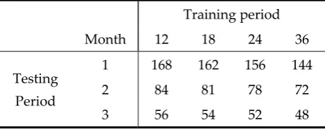
number of combinations of the data set. Table 2 shows the number of windows produced by a
295
several combinations of training and testing periods.
296
Table 2. Number of windows produced by the training and testing period between 2001 and 2015.
297
Training period
Month 12 18 24 36
Testing
Period
1 168 162 156 144
2 84 81 78 72
3 56 54 52 48
3.2. Pattern Matching by the Dynamic Time Warping Algorithm
298
A self-developed program was used for the analysis in Phase 2 with daily 10-minute time series
299
data. For pattern matching of daily market data by the dynamic time warping algorithm, two sets of
300
27 fixed patterns and 13 fixed patterns are used as input data. The daily market data between 9:00
301
am and 12:00 pm are assigned to one of the fixed patterns that is the most similar to the market data,
302
and then the frequency of each selected pattern is counted. For market data included in the training
303
period, the price at 12:00 pm is compared with the price of 10-minute intervals between 14:00 and
304
15:00. Then, the trading position is determined by the rule explained in Phase 2 in Section 2.3.
305
3.3. Trading Simulation
306
We conduct the trading simulation with various parameters. Figure 7 shows the PMTS user
307
interface, which displays the selected parameters for the trading simulation.
308
309
Figure 7. PMTS user interface.
310
311
The PMTS is operated using the two input files and six parameters. The two input files consist
312
of a fixed pattern file and a time series data file. The six input parameters used in our experiment are
313
as follows:
314
315
1. The training period for pattern matching: 3, 6, 9, 12, 18, 24, 36, 48, and 60 months are used.
316
2. Testing period for trading: 1, 2, and 3 months are used.
317
3. Filtering criteria: a value to exclude patterns if the frequency of a pattern assigned to daily
318
4. Stop-loss ratio: the rate of loss for the clearing position when the price moves against the
320
predicted direction. 0.5% is used.
321
5. U/D frequency: the proportion of “up” movements in the training period to determine the
322
trading position. Five values of 55%, 60%, 65%, 70%, 75%, and 80% are used.
323
6. Slippage cost: the level of slippage cost, where 0.02 pt is used.
324
325
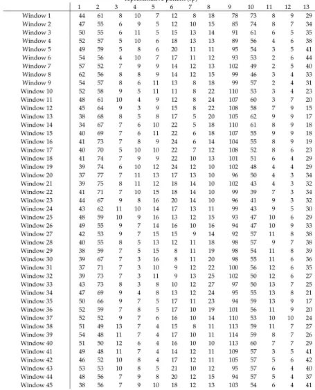
Table 3 shows the frequency of 13 representative patterns selected in each window with
326
18-month training and 3-month testing periods.
327
Table 3. Frequency of representative patterns for each window.
328
representative pattern (rp)
Window 46 34 62 5 9 9 21 10 15 102 52 9 4 39 Window 47 32 69 5 5 8 23 7 15 111 53 9 5 30 Window 48 31 67 5 3 9 24 8 18 107 57 7 4 29 Window 49 23 72 5 3 8 24 9 17 113 53 6 6 29 Window 50 26 72 4 4 7 27 6 16 113 52 5 7 30 Window 51 31 71 3 4 6 29 7 17 102 56 9 8 26 Window 52 32 72 5 4 7 27 7 15 100 55 6 7 30 Window 53 38 62 7 6 8 28 7 15 97 54 6 9 30 Window 54 36 58 10 6 7 25 5 16 102 52 7 8 37
329
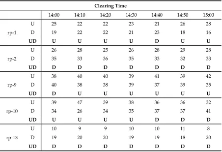
For example, testing is performed with patterns of rp-1, 2, 9, 10 and 13 in Window1 when the
330
filtering criterion is 20 ea. With the U/D frequency of 50%, the “up” or “down” position determined
331
and the frequency of “up” and “down” for this Window1 are reported in Table 4.
332
Table 4. Up or down position determined and the frequency of up and down for Window1 with
333
18-month training and 3-month testing periods, and 50% U/D frequency.
334
Clearing Time
14:00 14:10 14:20 14:30 14:40 14:50 15:00
rp-1
U 25 22 22 23 21 26 28
D 19 22 22 21 23 18 16
UD U U U U D U U
rp-2
U 26 28 25 26 28 29 28
D 35 33 36 35 33 32 33
UD D D D D D D D
rp-9
U 38 40 40 39 41 39 42
D 40 38 38 39 37 39 35
UD D U U U U U U
rp-10
U 39 47 39 38 36 36 32
D 34 26 34 35 37 37 41
UD U U U U D D D
rp-13
U 10 9 9 10 10 11 8
D 19 20 20 19 19 18 20
UD D D D D D D D
335
For example, the frequency of “up” for rp-1 at 14:00 is 25 and that of “down” is 19, so the
336
position is determined as “U” because the proportion of “up” is higher than 50%. However, as
337
shown in Table 5, when the 65% U/D frequency is used, it is classified as M (middle) rather than U or
338
D because the proportion of up (57%) was not higher than 65% and was not lower than 35%, i.e., it is
339
between 35% and 65%. In the case of where M is determined, no position is taken for testing.
340
341
342
343
Table 5. Up or down position determined and the frequency of up and down for Window1 with
345
18-month training and 3-month testing periods, and 65% U/D frequency.
346
Clearing Time
14:00 14:10 14:20 14:30 14:40 14:50 15:00
rp-1
U 25 22 22 23 21 26 28
D 19 22 22 21 23 18 16
UD M M M M M M M
rp-2
U 26 28 25 26 28 29 28
D 35 33 36 35 33 32 33
UD M M M M M M M
rp-9
U 38 40 40 39 41 39 42
D 40 38 38 39 37 39 35
UD M M M M M M M
rp-10
U 39 47 39 38 36 36 32
D 34 26 34 35 37 37 41
UD M M M M M M M
rp-13
U 10 9 9 10 10 11 8
D 19 20 20 19 19 18 20
UD D D D D D M D
3.4 PMTS Results
347
The PMTS is conducted as follows. We first calculated the annual return of the market data
348
clearing at 15:00 with various ranges of training and testing periods to find optimal periods. Given
349
these optimal periods, various filtering criteria and up/down frequency input parameters are used to
350
find optimal parameters. As a last step, we compared the annual returns clearing at every 10 minutes
351
from 14:00 to 15:00 using the optimal parameters determined in the previous steps to find the
352
optimal clearing time.
353
Various ranges of results are generated depending on the parameters used. With the results of
354
the simulation as described in Section 3.3, we repeat the experiments with significant parameters to
355
find the optimal parameters. The stop loss and slippage cost were fixed at 0.5% and 0.02 pt,
356
respectively, and other significant parameters are:
357
358
- Training period: 12, 18, 24, and 36 months
359
- Testing periods: 1, 2, and 3 months
360
- Filtering criteria: 5, 10, 15, and 20 ea
361
- U/D frequency: 65%, 70%, 75%, and 80%
362
363
To find the optimal parameters, we compare the Sharpe ratio produced by various ranges of
364
parameters when the trading position is cleared at every 10 minutes from 14:00 to 15:00. Table 6
365
shows the annual return, standard deviation, and Sharpe ratio of the market data clearing at 15:00
366
that is assigned to 13 fixed patterns with a 0.02 pt slippage cost, a 0.5% stop-loss ratio, a 20 ea filter
367
criteria, 65% U/D frequency, and a combination of training periods (12, 18, 24, and 36 months) and
368
testing periods (1, 2, and 3 months). Table 7 shows the annual return, standard deviation, and
369
Sharpe ratio of the market data clearing at 15:00 that is assigned to 13 fixed patterns with a 0.02 pt
370
slippage cost, a 0.5% stop-loss ratio, an 18-month training period, a 3-month testing period, and a
371
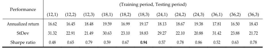
Taking the results in Table 6 and Table 7 together, the set of parameters that consists of a 0.02 pt
373
slippage cost, a 0.5% stop-loss ratio, an 18-month training period, a 3-month testing period, 20 ea
374
filtering criteria, and 65% U/D frequency were determined to have the highest Sharpe ratio of 0.94.
375
Table 6. Performance achieved from an experiment using 13 patterns with various combinations of
376
training and testing periods.
377
Performance
(Training period, Testing period)
(12,1) (12,2) (12,3) (18,1) (18,2) (18,3) (24,1) (24,2) (24,3) (36,1) (36,2) (36,3) Annualized
return 16.62 16.45 18.48 19.59 16.99 19.17 18.13 18.67 19.38 17.81 16.50 18.43 StDev 31.32 22.91 21.49 30.63 23.10 18.83 29.27 22.10 20.88 31.42 23.88 21.72 Sharpe ratio 0.48 0.65 0.79 0.59 0.67 0.94 0.57 0.78 0.86 0.52 0.63 0.78
Slippage Cost: 0.02 pt, Stop loss: 0.5%, Filter Criteria: 20, U/D Frequency: 65%, 15:00 exit.
378
Table 7. Performance achieved from an experiment using 13 patterns with various combinations of
379
filtering criteria and up/down frequencies.
380
Performance
(Filtering criteria, Up/Down frequency (%))
(5,65) (5,70) (5,75) (5,80) (10,65) (10,70) (10,75) (10,80) (15,65) (15,70) (15,75) (15,80) (20,65) (20,70) (20,75) (20,80) Annualized
return 18.83 1.30 0.63 0.69 18.27 0.91 0.12 0.32 19.17 0.69 0.06 0.09 19.17 0.25 -0.03 0.00 StDev 18.63 4.59 2.64 2.26 19.18 4.37 1.87 1.67 19.53 3.63 0.70 0.65 18.83 3.29 0.23 0.00 Sharpe ratio 0.93 -0.04 -0.33 -0.36 0.87 -0.14 -0.74 -0.71 0.90 -0.22 -2.07 -2.16 0.94 -0.38 -6.53 0.00
Slippage Cost: 0.02 pt, Stop loss: 0.5%, Training period: 18, Testing period: 3, 15:00 exit.
381
We conduct the same experiments using 27 fixed patterns as in the case of using 13 fixed
382
patterns. Table 8 shows the annual return, standard deviation, and Sharpe ratio of the market data
383
clearing at 15:00 that is assigned to 27 fixed patterns with a 0.02 pt slippage cost, a 0.5% stop-loss
384
ratio, 10 ea filter criteria, 65% U/D frequency, and a combination of training periods (12, 18, 24, and
385
36 months) and testing periods (1, 2, and 3 months). Table 9 shows the annual return, standard
386
deviation, and Sharpe ratio of the market data clearing at 15:00 that is assigned to 27 fixed patterns
387
with a 0.02 pt slippage cost, a 0.5% stop-loss ratio, a 24-month training period, a 3-month testing
388
period, and a combination of filtering criteria (5, 10, 15, and 20 ea) and U/D frequencies (65%, 70%,
389
75%, and 80%). Taking the results in Table 8 and Table 9 together, a set of parameters that consists of
390
a 0.02 pt slippage cost, a 0.5% stop-loss ratio, a 24-month training period, a 3-month testing period,
391
10 ea filtering criteria, and 65% U/D frequency is determined to have the highest Sharpe ratio of 0.76.
392
Table 8. Performance achieved from an experiment using 27 patterns with various combinations of
393
training and testing periods.
394
Performance
(Training period, Testing period)
(12,1) (12,2) (12,3) (18,1) (18,2) (18,3) (24,1) (24,2) (24,3) (36,1) (36,2) (36,3) Annualized return 16.62 16.45 18.48 19.59 16.99 19.17 18.13 18.67 19.38 17.81 16.50 18.43
StDev 31.32 22.91 21.49 30.63 23.10 18.83 29.27 22.10 20.88 31.42 23.88 21.72 Sharpe ratio 0.48 0.65 0.79 0.59 0.67 0.94 0.57 0.78 0.86 0.52 0.63 0.78
Slippage Cost: 0.02 pt, Stop loss: 0.5%, Filter Criteria: 10, U/D Frequency: 65%, 15:00 exit.
395
396
Table 9. Performance achieved from an experiment using 27 patterns with various combinations of
398
filtering criteria and up/down frequencies.
399
Performance
(Filtering criteria, Up/Down frequency (%))
(5,65) (5,70) (5,75) (5,80) (10,65) (10,70) (10,75) (10,80) (15,65) (15,70) (15,75) (15,80) (20,65) (20,70) (20,75) (20,80) Annualized return 18.54 1.26 0.25 0.09 18.66 1.09 0.01 -0.11 17.80 0.99 -0.01 0.00 18.25 1.20 -0.03 0.00
StDev 21.78 4.92 2.59 2.04 22.68 4.10 1.70 0.90 22.51 3.67 1.07 0.00 22.91 3.88 1.01 0.00 Sharpe ratio 0.78 -0.05 -0.48 -0.69 0.76 -0.10 -0.88 -1.79 0.72 -0.14 -1.42 0.00 0.73 -0.08 -1.52 0.00
Slippage Cost: 0.02 pt, Stop loss: 0.5%, Training period: 24, Testing period: 3, 15:00 exit.
400
We obtained experimental results from all possible combinations of parameters at every 10
401
minutes from 14:00 to 15:00. Table 10 and Table 11 report the annual return, standard deviation, and
402
Sharpe ratio of the market data clearing at every 10 minutes from 14:00 to 15:00 with the selected
403
parameters for using 13 and 27 fixed patterns, respectively.
404
Table 10. Performance achieved from an experiment using 13 patterns of clearing at every 10
405
minutes from 14:00 to 15:00.
406
Trading exit time 1400 1410 1420 1430 1440 1450 1500 Avg.
Annualized return 7.24 11.42 13.07 13.80 17.65 18.05 19.17 14.34 StDev 21.05 20.41 18.78 21.33 23.15 24.61 18.83 21.17
Sharpe Ratio 0.27 0.49 0.62 0.58 0.70 0.67 0.94 0.61
Slippage Cost: 0.02 pt, Stop loss: 0.5%, Training period: 18, Testing period: 3, Filter Criteria: 20, U/D Frequency: 65%.
407
Table 11. Performance achieved from an experiment using 27 patterns of clearing at every 10
408
minutes from 14:00 to 15:00.
409
Trading exit time 1400 1410 1420 1430 1440 1450 1500 Avg.
Annualized return 7.25 10.93 12.72 13.39 15.52 17.64 18.66 13.73
StDev 19.31 20.40 22.88 19.18 22.13 23.40 22.68 21.43 Sharpe Ratio 0.30 0.46 0.49 0.62 0.63 0.69 0.76 0.56
Slippage Cost: 0.02 pt, Stop loss: 0.5%, Training period: 24, Testing period: 3, Filter Criteria: 10, U/D Frequency: 65%.
410
As shown in Table 6-Table 9, the performance of the market data clearing at 15:00 is found to be
411
the best. We also compare the performance of the market data in the experiments using 13 and 27
412
fixed patterns. The average values of the annual return, standard deviation, and Sharpe ratio of the
413
market data clearing at every 10 minutes from 14:00 to 15:00 are reported in the last column in Table
414
10 and Table 11. The average Sharpe ratio for the experiments using 13 fixed patterns (0.61) is higher
415
than that for experiments using 27 fixed patterns (0.56). We also find that the best performance with
416
Sharpe ratio of 0.94 is produced by the experiment using 13 fixed patterns and clearing at 15:00. In
417
addition, we calculate the average of total profit obtained when the optimal parameters are used in
418
an experiment using 13 and 27 patterns of clearing at every 10 minutes from 14:00 to 15:00. Table 12
419
shows the average of the total profit points in an experiment using 13 and 27 patterns of clearing at
420
every 10 minutes from 14:00 to 15:00 with the selected parameters.
421
Table 12. Average of total profit in an experiment using 13 and 27 patterns of clearing at every 10
428
minutes from 14:00 to 15:00.
429
Avg. of total profit (pt) 1400 1410 1420 1430 1440 1450 1500 avg.
13 pattern1 3.62 5.71 6.53 6.90 8.83 9.02 9.58 7.17
27 pattern2 3.63 5.46 6.36 6.69 7.76 8.82 9.33 6.87
1 Slippage Cost: 0.02 pt, Stop loss: 0.5%, Training period: 18, Testing period: 3, Filter Criteria: 20, U/D Frequency: 65%.
430
2Slippage Cost: 0.02 pt, Stop loss: 0.5%, Training period: 24, Testing period: 3, Filter Criteria: 10, U/D Frequency: 65%.
431
As shown in Table 12, the average total profit is the highest (9.58 pt) when the experiment uses
432
13 fixed patterns and clears at 15:00.
433
Figure 8 and Figure 9 show the average returns of the market data that are assigned to each of
434
the 27 and 13 representative patterns for all combinations of parameters used in this study of
435
clearing at every 10 minutes from 14:00 to 15:00, respectively. Most patterns show higher returns at
436
the 15:00 clearing time.
437
438
Figure 8. Average return from the experiment with 27 patterns by clearing time.
439
440
441
Figure 9. Average return from the experiment with 13 patterns by clearing time.
442
4. Discussion
443
The purpose of this study is to develop a pattern matching trading system using the DTW
444
algorithm with optimal parameters. Using KOSPI 200 index futures market data from 2001 to 2015,
445
experimental results show that the PMTS based on the DTW algorithm provides stable and effective
447
trading strategies with relatively low trading frequencies.
448
A number of financial instruments that are traded in financial markets exist, and an enormous
449
number of models or techniques have been developed for efficient investment strategies. Therefore,
450
financial instruments and investment techniques as well as investors have played an important role
451
in sustaining financial markets. Investor communities that have sustained financial markets are able
452
to make more efficient investments by using the PMTS. In this sense, the system developed in this
453
paper is a sustainable investment technique and helps financial markets to achieve efficient
454
sustainability.
455
A future study can be enriched by the studies presented in this paper. An interesting extension
456
to the current study would include empirical studies using a more sophisticated DWP algorithm,
457
such as the deepening dynamic time warping (DDTW) algorithm or the segmented dynamic time
458
warping (SDTW) algorithm or the cluster generative statistical dynamic time warping (CSDTW)
459
algorithm, from which better results are expected. This study could also be extended by experiments
460
with various financial instruments such as interest rate futures contracts, options, and other
461
derivatives to find the optimal strategy.
462
References
463
1. BIRĂU, F.R. Financial Derivatives-Meanings Beyond Subprime Crisis Stigma. Analele Universităţii
464
Constantin Brâncuşi din Târgu Jiu: Seria Economie2010, 2(4), 195-199.
465
2. Carmassi, J., Gros, D., & Micossi, S. The global financial crisis: Causes and cures. JCMS: Journal of Common
466
Market Studies 2009, 47(5), 977-996.
467
3. Crotty, J. Structural causes of the global financial crisis: a critical assessment of the ‘new financial
468
architecture’. Cambridge journal of economics2009, 33(4), 563-580.
469
4. Ghysels, E., & Seon, J. The Asian financial crisis: The role of derivative securities trading and foreign
470
investors in Korea. Journal of international Money and Finance2005, 24(4), 607-630.
471
5. Caillault, É. P., Lefebvre, A., & Bigand, A. Dynamic time warping-based imputation for univariate time
472
series data. Pattern Recognition Letters2017.
473
6. Kwon, D., & Lee, T. Hedging effectiveness of KOSPI200 index futures through VECM-CC-GARCH model.
474
Journal of the Korean Data and Information Science Society2014, 25(6), 1449-1466.
475
7. Keogh, E. J., Pazzani, M. J. Scaling up dynamic time warping to massive datasets. In European Conference
476
on Principles of Data Mining and Knowledge Discovery. Springer, Berlin, Heidelberg, 1999, Aug;
477
(pp.1-11).
478
8. Senin, P. Dynamic time warping algorithm review. Information and Computer Science Department
479
University of Hawaii at Manoa Honolulu, USA, 855, 1-23.
480
9. Agrawal, R., Faloutsos, C., & Swami, A. Efficient similarity search in sequence databases. In International
481
conference on foundations of data organization and algorithms, Springer, Berlin, Heidelberg, 1993, Oct;
482
(pp.69-84).
483
10. Das, G., Gunopulos, D., & Mannila, H. Finding similar time series. In European Symposium on Principles
484
of Data Mining and Knowledge Discovery, Springer, Berlin, Heidelberg, 1997, Jun; (pp.88-100).
485
11. Fu, T. C., Chung, F. L., Luk, R., & Ng, C. M. Stock time series pattern matching: Template-based vs.
486
rule-based approaches. Engineering Applications of Artificial Intelligence 2007, 20(3), 347-364.
487
12. Bagheri, A., Peyhani, H. M., & Akbari, M. Financial forecasting using ANFIS networks with
488
quantum-behaved particle swarm optimization. Expert Systems with Applications2014, 41(14), 6235-6250.
489
13. Patel, J., Shah, S., Thakkar, P., & Kotecha, K. Predicting stock and stock price index movement using trend
490
deterministic data preparation and machine learning techniques. Expert Systems with Applications2015,
491
42(1), 259-268.
492
14. Deboeck, G. Trading on the edge: neural, genetic, and fuzzy systems for chaotic financial markets. John
493
Wiley & Sons, 1994; Volume 39.
494
15. Leigh, W., Modani, N., & Hightower, R. A computational implementation of stock charting: abrupt
495
volume increase as signal for movement in New York stock exchange composite index. Decision Support
496
Systems2004, 37(4), 515-530.
497
16. Leigh, W., Modani, N., Purvis, R., & Roberts, T. Stock market trading rule discovery using technical
498
17. Leigh, W., Purvis, R., & Ragusa, J. M. Forecasting the NYSE composite index with technical analysis,
500
pattern recognizer, neural network, and genetic algorithm: a case study in romantic decision support.
501
Decision support systems2002, 32(4), 361-377.
502
18. Lo, A. W., Mamaysky, H., & Wang, J. Foundations of technical analysis: Computational algorithms,
503
statistical inference, and empirical implementation. The journal of finance2000, 55(4), 1705-1765.
504
19. Chen, T. L., & Chen, F. Y. An intelligent pattern recognition model for supporting investment decisions in
505
stock market. Information Sciences2016, 346, 261-274.
506
20. Chung, F. L., Fu, T. C., Ng, V., & Luk, R. W. An evolutionary approach to pattern-based time series
507
segmentation. IEEE transactions on evolutionary computation2004, 8(5), 471-489.
508
21. Dong, M., & Zhou, X. S. Exploring the fuzzy nature of technical patterns of US stock market. Proceedings of
509
Fuzzy System and Knowledge Discovery2002, 1, 324-328.
510
22. Kim, S. D., Lee, J. W., Lee, J., & Chae, J. A two-phase stock trading system using distributional differences.
511
In International Conference on Database and Expert Systems Applications, Springer, Berlin, Heidelberg,
512
2002, Sep; (pp.143-152).
513
23. Hu, Y., Feng, B., Zhang, X., Ngai, E. W. T., & Liu, M. Stock trading rule discovery with an evolutionary
514
trend following model. Expert Systems with Applications2015, 42(1), 212-222.
515
24. de Oliveira, F. A., Nobre, C. N., & Zárate, L. E. Applying Artificial Neural Networks to prediction of stock
516
price and improvement of the directional prediction index–Case study of PETR4, Petrobras, Brazil. Expert
517
Systems with Applications2013, 40(18), 7596-7606.
518
25. Lee, S. J., Ahn, J. J., Oh, K. J., & Kim, T. Y. Using rough set to support investment strategies of real-time
519
trading in futures market. Applied Intelligence2010, 32(3), 364-377.
520
26. Lee, S. J., Oh, K. J., & Kim, T. Y. How many reference patterns can improve profitability for real-time
521
trading in futures market?. Expert Systems with Applications 2012, 39(8), 7458-7470.
522
27. Berndt, D. J., & Clifford, J. Using dynamic time warping to find patterns in time series. In KDD workshop,
523
1994, Jul; (Vol. 10, No. 16, pp. 359-370).
524
28. Bellman, R., & Kalaba, R. On adaptive control processes. IRE Transactions on Automatic Control1959, 4(2),
525
1-9.
526
29. Myers, C., Rabiner, L., & Rosenberg, A. Performance tradeoffs in dynamic time warping algorithms for
527
isolated word recognition. IEEE Transactions on Acoustics, Speech, and Signal Processing1980, 28(6), 623-635.
528
30. Sakoe, H., & Chiba, S. Dynamic programming algorithm optimization for spoken word recognition. IEEE
529
transactions on acoustics, speech, and signal processing1978, 26(1), 43-49.
530
31. Kuzmanic, A., & Zanchi, V. Hand shape classification using DTW and LCSS as similarity measures for
531
vision-based gesture recognition system. In EUROCON, 2007. The International Conference on" Computer
532
as a Tool" (pp. 264-269). IEEE.
533
32. Corradini, A. Dynamic time warping for off-line recognition of a small gesture vocabulary. In Recognition,
534
Analysis, and Tracking of Faces and Gestures in Real-Time Systems, 2001. Proceedings. IEEE ICCV
535
Workshop on (pp. 82-89). IEEE.
536
33. Niennattrakul, V., & Ratanamahatana, C. A. On clustering multimedia time series data using k-means and
537
dynamic time warping. 2007, Apr; (pp. 733-738). IEEE.
538
34. Bahlmann, C., & Burkhardt, H. The writer independent online handwriting recognition system frog on
539
hand and cluster generative statistical dynamic time warping. IEEE Transactions on Pattern Analysis and
540
Machine Intelligence2004, 26(3), 299-310.
541
35. Kahveci, T., & Singh, A. Variable length queries for time series data. In Data Engineering, 2001.
542
Proceedings. 17th International Conference on (pp. 273-282). IEEE.
543
36. Kahveci, T., Singh, A., & Gurel, A. Similarity searching for multi-attribute sequences. In Scientific and
544
Statistical Database Management, 2002. Proceedings. 14th International Conference on (pp. 175-184). IEEE.
545
37. Müller, M., Mattes, H., & Kurth, F. An efficient multiscale approach to audio synchronization. In ISMIR,
546
2006, Oct; (pp. 192-197).
547
38. Müller, M. Dynamic time warping. Information retrieval for music and motion2007, 69-84.
548
39. Salvador, S., & Chan, P. Toward accurate dynamic time warping in linear time and space. Intelligent Data
549
Analysis 2007, 11(5), 561-580.
550
40. Jang, G. S., Lai, F., Jiang, B. W., Parng, T. M., & Chien, L. H. Intelligent stock trading system with price
551
trend prediction and reversal recognition using dual-module neural networks. Applied Intelligence 1993,
552
3(3), 225-248.
553
41. Hwarng, H. B. Insights into neural-network forecasting of time series corresponding to ARMA (p, q)
554
42. Ahn, J. J., Kim, D. H., Oh, K. J., & Kim, T. Y. Applying option Greeks to directional forecasting of implied
556
volatility in the options market: An intelligent approach. Expert Systems with Applications 2012, 39(10),
557
9315-9322.
558
43. Ahn, J. J., Byun, H. W., Oh, K. J., & Kim, T. Y. Using ridge regression with genetic algorithm to enhance
559
real estate appraisal forecasting. Expert Systems with Applications2012, 39(9), 8369-8379.
560
44. Chou, J. S., & Ngo, N. T. Time series analytics using sliding window metaheuristic optimization-based
561
machine learning system for identifying building energy consumption patterns. Applied energy2016, 177,
562
751-770.
563
45. Chang, E. C. Returns to speculators and the theory of normal backwardation. The Journal of Finance1985,
564
40(1), 193-208.
565
46. Hartzmark, M. L. Returns to individual traders of futures: Aggregate results. Journal of Political Economy
566
1987, 95(6), 1292-1306.
567
47. Hartzmark, M. L. Luck versus forecast ability: Determinants of trader performance in futures markets.
568
Journal of Business1991, 49-74.
569
48. Leuthold, R. M., Garcia, P., & Lu, R. The returns and forecasting ability of large traders in the frozen pork
570
bellies futures market. Journal of Business1994, 459-473.
571
49. Wang, C. Investor sentiment and return predictability in agricultural futures markets. Journal of Futures