The Sensitivity of Tropical Cyclone Simulations in the WRF Model to Surface Layer and Planetary Boundary Layer Parameterization

ABSTRACT

HILL, KEVIN ANTHONY. The Sensitivity of Tropical Cyclone Simulations in the WRF

Model to Surface Layer and Planetary Boundary Layer Parameterization. (Under the

direction of Dr. Gary M. Lackmann).

The high wind speeds found in tropical cyclones fundamentally change the

physical processes by which heat, moisture and momentum are transferred between the

ocean and the lower atmosphere. Despite this fact, surface and boundary layer

parameterization schemes in many numerical models that are frequently used for tropical

cyclone simulations are based on assumptions made in more tranquil atmospheric

conditions. Limited observations in the high wind speed conditions found in strong

tropical cyclones suggest that spray and foam can enhance the transfer of heat and

moisture from the ocean to the atmosphere, while reducing drag. Inclusion of the effects

due to sea spray in a numerical model leads to stronger tropical cyclones (Wang et al.

2001, Perrie et al. 2005).

Based upon the absence of sea spray effects and the values of the exchange

coefficients in the WRF model, it was anticipated that simulations using an idealized

vortex and ambient environment would not reach the thermodynamically estimated

theoretical maximum intensity (MPI) limit of Emanuel (1986). In addition, it was

parameterization choice. Grid spacing was also hypothesized to impact the simulated TC

intensity, with the expectation that simulations with smaller grid spacing would produce

more intense TCs, based on the results of previous studies.

Simulated TC intensity is found to be highly sensitive to model grid spacing in

experiments with Hurricane Ivan or with an idealized initial vortex. Simulations using

4-km grid spacing were able to produce TCs that exceeded the MPI of the idealized

environment (determined by minimum sea level pressure), while simulations using

coarser (12 or 36-km) grid spacing were not. Simulations of Hurricane Ivan using 4-km

grid spacing, initialized with a vortex that was ~60 hPa weaker than observations reached

the maximum intensity of the observed system, and exceeded the observed intensity

during the latter stages of the simulation. These results suggest that the WRF model, in

its current configuration, overestimates TC intensity, especially with small values of

horizontal grid spacing. If the exchange of moisture, heat and momentum were adjusted

to more accurately portray the conditions found in high wind speed conditions, the

idealized tropical cyclone would likely exceed the theoretical MPI by an even larger

amount. Therefore, it is concluded that some other aspect of the model formulation may

lead to an overestimation of tropical cyclone intensity, or that there are deficiencies in

MPI theory.

The Sensitivity of Tropical Cyclone Simulations in the WRF Model to Surface Layer

and Planetary Boundary Layer Parameterization.

By

Kevin Anthony Hill

A thesis submitted to the Graduate Faculty of

North Carolina State University

in partial fulfillment of the requirements for the Degree of

Master of Science

MARINE, EARTH, AND ATMOSPHERIC SCIENCES

Raleigh

2006

APPROVED BY:

Dr. Gary M. Lackmann

(Chair of Advisory Committee)

BIOGRAPHY

Kevin was born in Buffalo, NY on 11 November 1982, and graduated from

Clarence High School in 2000. Kevin’s first fascination with meteorology was with lake

effect snowstorms, which dump large amounts of snow in very isolated areas. Living

north of the typically hard hit locations, Kevin would often wonder why his hometown

would often be spared the heaviest snow, while young men in other towns would be

blessed with copious amounts snow (and, more importantly, days off of school). The

first meteorology lesson that Kevin learned was that wind circulated in a

counter-clockwise direction around low-pressure systems. Often, the location of the low pressure

systems passing to the north of WNY would dictate precisely how the winds lined up

across Lake Erie, and whether or not Kevin would have to go to school. On the other

extreme of meteorological phenomenon, Kevin became interested in tropical cyclones as

well. In the days before vast amounts of data were available to the public on the internet,

Kevin would make sitting in front of the television at 50 past the hour to watch the

Weather Channel’s tropical update a priority during times of tropical activity.

During high school, Kevin learned that he had an aptitude for math and science,

and upon arriving at The State University of New York at Brockport, he chose to major

in meteorology and minor in math and statistics, while taking additional courses in

physics and computer science in order to prepare for graduate school. During his senior

year, Kevin got his first taste of research by performing a senior seminar project

mathematics and statistics, Kevin began graduate school in Atmospheric Science at

NCSU under the advisement of Dr. Gary. M. Lackmann in the fall of 2004. Kevin

benefited from a flexible research topic and an advisor willing to tailor the project to his

interests, allowing the research to remain intriguing and fresh throughout its course of

development. Kevin presented his preliminary research results on “Steady-state

ACKNOWLEDGEMENTS

I would like to thank the members of my advisory committee, Drs. Gary

Lackmann, Lian Xie, and Sethu Raman, for their insights and helpful suggestions. I

would especially like to thank Dr. Gary Lackmann for allowing me the opportunity to

choose a research topic that was of particular interest to me. It has truly been a pleasure

working on this project under his advisement, and I feel incredibly lucky to have been

accepted into his research group. I hope he is happy with his decision!

My friends are also acknowledged for providing activities that got my mind off of

the large amount of work that lay before me! I have truly enjoyed my graduate

TABLE OF CONTENTS

Page

LIST OF TABLES

xi

LIST OF FIGURES

xii

1) INTRODUCTION

1

1.1) Motivation

1

1.2) Literature Review

4

1.2.1) TC Energetics: Initial Theory, and Oceanic Influence

4

1.2.2) The Surface Layer in a Hurricane: Theory, Modeling, and Observations 6

1.2.3) The PBL in a Hurricane: Theory, Modeling, and Observations 12

1.2.4) Maximum Potential Intensity (MPI) Theory

14

1.2.5) Literature Review Summary

20

1.3) Hypotheses

21

1.4) Thesis Outline

23

2) METHODOLOGY

27

2.1) Weather Research and Forecasting Model Version 2.1.2

27

2.1.1) Model Description

27

2.1.2) Initial and Boundary Conditions

27

2.1.3) Physics Options in All Simulations

28

2.1.4) Planetary Boundary Layer Schemes

30

2.1.4.1) Yonsei-University (YSU)

30

2.1.5.1) Scheme Used with YSU PBL

32

2.1.5.2) Scheme Used with MYJ PBL

33

2.2) Initial and Boundary Conditions

35

2.2.1) Idealized Model Experiments

35

2.2.1.1) Lateral Boundary Conditions

36

2.2.1.2) Initial Vortex

37

2.2.1.2.1) Blending the Eye and Ambient Temperature Profiles 38

2.2.1.2.2) Calculation of Sea Level Pressure and Height

39

2.2.1.2.3) Calculating Wind Speed

42

2.2.1.3) Model Configuration of Idealized Simulations

43

2.2.2) Hurricane Ivan Experiments

44

2.3) Model Simulation Analysis

45

2.3.1) TC Intensity

45

2.3.2) TC Track

46

2.3.3) Area Averaged Values

46

2.3.4) Azimuthal Averaging

46

2.3.5) RMW, Radius of TS and Hurricane Force Wind

47

2.3.6) Surface Layer Exchange Coefficients

47

2.3.7) Fluxes and Exchange Coefficients as a Function of Wind Speed

49

2.3.8) Time Averaging

49

3) HURRICANE IVAN (2004)

61

3.1) Storm Information

61

3.2) Does WRF Produce a Realistic TC Structure 62

3.3) Time-series of Model Parameters

64

3.3.1) Track

64

3.3.2) Intensity

64

3.3.2.1) Minimum Sea Level Pressure (MSLP)

64

3.3.3) Values of Fluxes Produced by Surface Layer Parameterization

68

3.3.3.1) Latent Heat Flux (LHFLX)

68

3.3.3.2) Sensible Heat Flux (HFLX)

69

3.3.4) Precipitation Amount

70

3.4) Sensitivity of MYJ Simulations to Vertical Resolution

71

3.4.1) Track

71

3.4.2) Intensity

72

3.4.3) Difference in Area-Averaged LHFLX and HFLX

73

3.4.4) Sensitivity to Vertical Resolution Summary

74

3.5) Wind Speed Dependence of Surface Layer Parameters

75

3.5.1) Latent Heat Flux (LHFLX)

76

3.5.2) Exchange Coefficient for Moisture (Cq)

77

3.5.3) Sensible Heat Flux (HFLX)

79

3.5.4) Exchange Coefficient for Sensible Heat (Ck)

79

3.5.5) Roughness Length

81

3.5.6) Exchange Coefficient for Momentum (Cd)

81

3.5.7) Ratio Ck/Cd .

81

3.6) Time-Averaged Structure

82

3.6.1) Storm Structure During Averaging Period

83

3.6.1.1) Maximum 10-m Wind and MSLP

83

3.6.1.2) Simulated Radar Structure

83

3.6.1.3) Precipitation Structure

84

3.6.2) Time and Azimuthally-Averaged 2-D Horizontal Structure

84

3.6.2.1) Sea Level Pressure (SLP)

85

3.6.2.2) 10-m Wind Speed

85

3.6.2.3) Latent Heat Flux (LHFLX)

86

3.6.2.4) Sensible Heat Flux (HFLX)

86

3.6.3) Time and Azimuthally-Averaged 3-D Structure

87

3.6.3.1) Vertical Motion

88

3.6.3.2) Specific Humidity

89

3.6.3.3) Wind Speed

90

3.6.3.3.1) Normalized Profiles and Comparison with

90

Observations

3.6.3.3.2) Cross Sections of Tangential Velocity

91

3.6.3.3.3) Velocity Tendency due to PBL parameterization 91

3.6.3.4) Potential Temperature

92

3.6.3.4.1) Potential Temperature Tendency due to PBL

Parameterization

93

3.7) General Conclusions Regarding Ivan Simulations

93

4) IDEALIZED EXPERIMENTS

159

4.1) WRF Model Simulation Overview

160

4.1.1) Intensity

161

4.1.1.1) Minimum SLP

161

4.1.1.2) Maximum 10-m Wind Speed

161

4.1.2) Values of Fluxes Produced by Surface Layer Parameterization

163

4.1.2.1) Latent Heat Flux

163

4.1.2.2) Sensible Heat Flux

164

4.1.3) Precipitation Amount

165

4.2) Storm Structure Change

165

4.2.1) Sea Level Pressure Distribution

166

4.2.2) 10-m Wind Distribution

167

4.2.3) Radius of Maximum, Tropical Storm, and Hurricane Force Wind Radii

167

4.2.4) Comparison of Size with Observed TCs

168

4.2.5) Pressure and Wind Relationship

169

4.2.6) Summary of Structure Change

170

4.3.1) Latent Heat Flux

171

4.3.2) Exchange Coefficient for Moisture

172

4.3.3) Sensible Heat Flux

173

4.3.4) Exchange Coefficient for Sensible Heat

173

4.3.5) Roughness Length

174

4.3.6) Exchange Coefficient for Momentum

174

4.3.7) Ratio Ck/Cd

174

4.4) Time-Averaged Structure

175

4.4.1) Storm Structure during Averaging Period

176

4.4.1.1) SLP and 10-m Wind Distribution

176

4.4.1.2) Simulated Radar Structure

177

4.4.1.3) Precipitation Structure

178

4.4.2) Time and Azimuthally-Averaged 2-D Horizontal Structure

179

4.4.2.1) Sea Level Pressure

179

4.4.2.2) 10-m Wind Speed

179

4.4.2.3) Latent Heat Flux

180

4.4.2.4) Sensible Heat Flux

181

4.4.3) Time and Azimuthally-Averaged 3-D Structure

181

4.4.3.1) Vertical Motion

182

4.4.3.1.1) Downward Vertical Motion Cross Sections

182

4.4.3.1.2) Upward Vertical Motion Cross Sections

182

4.4.3.2) Specific Humidity

183

4.4.3.3) Wind Speed

184

4.4.3.3.1) Normalized Profiles and Comparison with

184

Observations

5) CONCLUSIONS AND FUTURE RESEARCH

242

5.1) Overview

242

5.2) Review of Hypotheses

243

5.3) Comparison of Simulated and Theoretical Maximum Intensity

243

5.4) Comparison of Simulated and Observed Intensity for Hurricane Ivan

244

5.5) Sensitivity to Grid Spacing

244

5.6) Sensitivity to Surface Layer Parameterization

245

5.7) Sensitivity to PBL Parameterization

246

5.8) Summary and Future Work

247

LIST OF TABLES

Page

TABLE 3.1 List of simulation names for Ivan simulations

98

TABLE 3.2 Average track-forecast error (km) for many different forecast models

and the NHC official forecast. Error listed in km, with the number of

cases in parentheses

98

TABLE 3.3 Track errors (in km) for Ivan simulations

99

TABLE 3.4 492-km area-averaged values from time averaged TCs

95

TABLE 4.1 List of simulation names for idealized simulations

190

TABLE 4.2 Simulation hours of maximum 10-m wind speed and minimum sea

level pressure (MSLP). MSLP values exceeding theoretical MPI

in bold

190

LIST OF FIGURES

Page

FIG. 1.1. Official National Hurricane Center intensity forecast error, for the

period 1990 – 1997. From Avila, 1998

25

FIG. 1.2. Exchange coefficients for drag (CD, in blue) and heat (CK, in green).

From Large and Pond (1982)

25

FIG. 1.3. Schematic of the PBL structure in a mature hurricane.

From Anthes, 1982

26

FIG. 2.1. Mean hurricane season temperature profile as calculated by Jordan

(1958) (red curve) and best-fit logarithmic regression equation

(black curve). Equation based on temperature values below the

tropopause (below ~ 110 hPa)

51

FIG. 2.2. Mean hurricane season temperature profile as calculated by Jordan

(1958) (red curve) and best-fit logarithmic regression equation

(black curve). Equation based on temperature values above the

tropopause (above ~ 110 hPa)

51

FIG. 2.3. Mean hurricane season temperature profile as calculated by Jordan

(1958) (red curve) and best-fit curve using regression equation

from FIG 2.1 below 100 hPa and regression equation from FIG 2.2

above 100 hPa (black curve)

52

FIG. 2.4. Mean temperature profile for hurricane eye from hurricanes with

central pressure less than 995 hPa, as calculated by Sheets (1958)

(blue curve), and best-fit logarithmic regression equation (black curve).

Equation based on temperature values below the tropopause

(below ~ 110 hPa)

53

FIG. 2.5. Mean temperature profile for hurricane eye from hurricanes with

central pressure less than 995 hPa, as calculated by Sheets (1958)

(blue curve), and best-fit logarithmic regression equation (black curve).

Equation based on temperature values above the tropopause

FIG. 2.6. Mean temperature profile for hurricane eye from hurricanes with

central pressure less than 995 hPa, as calculated by Sheets (1958)

(blue curve), and best-fit curve using regression equation from FIG 2.4

below 110 hPa and regression equation from FIG 2.5 above 110 hPa

(black curve)

54

FIG. 2.7. Comparison of the temperature sounding in the eye (blue curve) and in

the ambient environment (red curve)

55

FIG. 2.8. Value of the scaling parameter for the temperature anomalies (y-axis)

plotted versus the radial distance from the storm center (x-axis) in km 56

FIG. 2.9. Cross section of temperature (in Kelvin, represented by colors) and

radial distance from center plotted in dashed lines (in kilometers). Note

that this plot was created before the calculation of surface pressure, and

values near the center that are higher than the central pressure would thus be

invalid. Cross-section taken from west to east (8 degrees total width) through

center of idealized vortex

56

FIG. 2.10. Column averaged virtual temperature (colors) in Kelvin and distance from

storm center (contours) in km

57

FIG. 2.11. Height anomaly (colors) in meters defined as the 20 hPa height minus the

height of the 20 hPa surface in the Jordan mean sounding. Positive values

indicate a higher 20 hPa height than in the Jordan mean

atmosphere sounding

57

FIG. 2.12. Sea level pressure in hPa (shaded) and distance from vortex center in km

(contoured)

58

FIG. 2.13. Height (in meters) of the following pressure surfaces: 1000 hPa (upper left),

850 hPa (upper right), 750 hPa (lower left) and 500 hPa (lower right) 58

FIG. 2.14. Tangential component of the wind in mph on a west-east cross section made

From the vortex center extending eastward. Shading represents wind speed,

contours the distance from the storm center in km

59

FIG. 2.15. Initial location of domains in idealized simulations

60

FIG. 2.16. Initial location of domains in simulations of Ivan

60

FIG. 3.1. TPC best track for Hurricane Ivan (2004)

100

FIG. 3.3. Model simulated radar reflectivity from IMYJ4 simulation, hour 72, valid

at 00 UTC 14 September 2004

102

FIG. 3.4. Radar reflectivity image of Hurricane Ivan from the Mobile, AL National

Weather Service Forecast Office WSR-88D Doppler radar at 0702 UTC 16

September 2004

103

FIG. 3.5. Model simulated radar reflectivity from IMYJ4 simulation, hour 126,

valid at 06 UTC 16 September 2004

104

FIG. 3.6. The track of Ivan 1) as analyzed by the NHC (in black), 2) produced using

the IMYJ36 simulation (in blue) and 3) produced using the IYSU36 simulation

(in red). Track is shown from 00 UTC 11 September 2004 – 00 UTC 17

September 2004, and begins at the lower-right corner of the figure 105

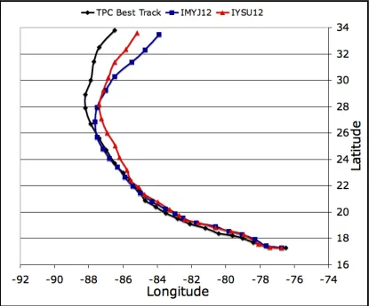
FIG. 3.7. Same as in fig. 3.6, except for IMYJ12 (blue) and IYSU12 (red) 106

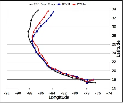
FIG. 3.8. Same as in fig 3.6 except for IMYJ4 (blue) and IYSU4 (red)

107

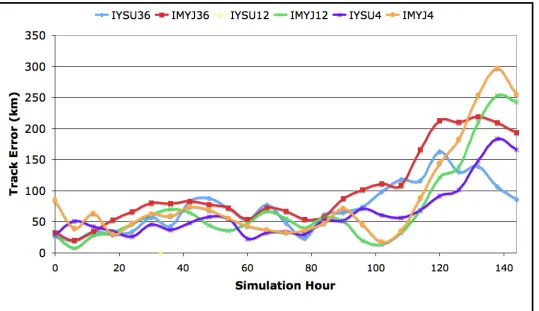
FIG. 3.9. Time-series of track error for Ivan simulations (km)

108

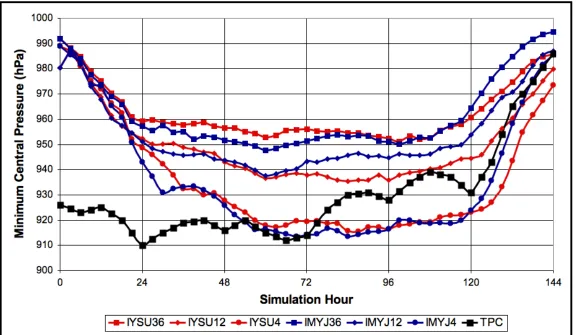
FIG. 3.10. Time-series of 1) the model simulated central pressure from WRF (3-hourly)

and 2) the analyzed central pressure from NHC (6-hourly) for Ivan

simulations

109

FIG. 3.11. Time-series of the minimum sea level pressure departure, calculated as

actual minimum central pressure subtracted from the simulated minimum

central pressure for Ivan simulations

110

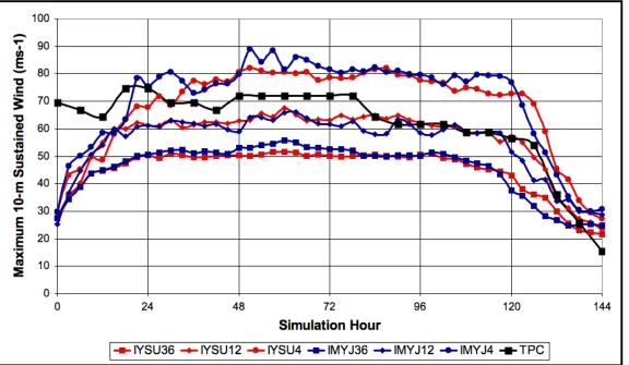
FIG. 3.12. Time-series of 1) the model simulated maximum 10-m winds (3-hourly)

and 2) the analyzed maximum 10-m winds from NHC (6-hourly) for Ivan

simulations

111

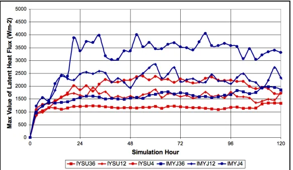
FIG. 3.13. Time-series of the maximum value of latent heat flux (y-axis, in Wm

₎

for Ivan simulations

112

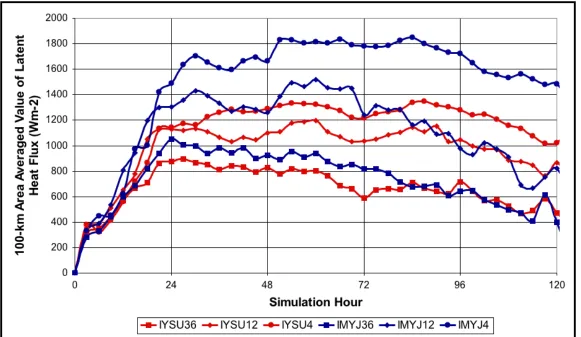
FIG. 3.14. Time-series of the storm-centered 100-km area-averaged value of latent heat

flux (y-axis, in Wm

) for Ivan simulations

113

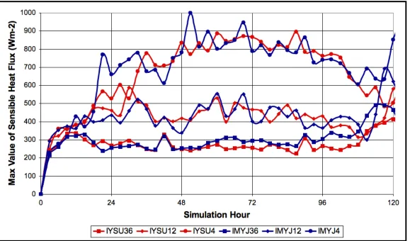
FIG. 3.16. Time-series of the storm-centered 100-km area-averaged value of sensible

heat flux (y-axis, in Wm

) for Ivan simulations

115

FIG. 3.17. Time-series of the storm-centered 400-km area-averaged hourly precipitation

for IYSU36 (in red) and IMYJ36 (blue) and the normalized value (MYJ/YSU)

in green

116

FIG. 3.18. Same as in fig. 3.17, except for domain 2

117

FIG. 3.19. Same as in fig. 3.17, except for domain 3

118

FIG. 3.20. The track of Ivan 1) as analyzed by the NHC (in black), 2) produced using

the IMYJ36 simulation (in blue) and 3) produced using the IMYJM36

simulation (in red). Track is shown from 00 UTC 11 September 2004 –

00 UTC 17 September 2004, and begins at the lower-right corner of the

figure 119

FIG. 3.21. Same as in figure 3.20, but for IMYJ12 (blue) and IMYJM12 (red) 120

FIG. 3.22. Same as in figure 3.20, but for IMYJ4 (blue) and IMYJM4 (red) 121

FIG. 3.23. Time-series of the difference in minimum central pressure (blue, in hPa) and

and maximum 10-m wind (red, in ms

) between the IMYJ36 and

IMYJM36 simulations

122

FIG. 3.24. Same as in fig. 3.23, but for the IMYJ12 and IMYJM12 simulations 123

FIG. 3.25. Same as in fig. 3.23 except for the IMYJ4 and IMYJM4 simulations 124

FIG. 3.26. Time-series of the difference in the 100-km area-averaged LHFLX

Between the IMYJM and IMYJ simulations (Wm

). Domain indicated

in legend

125

FIG. 3.27. Percent difference in the 100-km area-averaged LHFLX between the

IMYJM and IMYJ simulations. Domain indicated in legend 126

FIG. 3.28. Time-series of the difference in the 100-km area-averaged HFLX between

the IMYJM and IMYJ simulations (Wm

). Domain indicated in legend 127

FIG. 3.29. Percent difference in the 100-km area-averaged HFLX between the

IMYJM and IMYJ simulations. Domain indicated in legend 128

FIG. 3.30. Model latent heat flux (Wm

) as a function of wind speed (ms

). IYSU4

FIG. 3.31. Same as in fig. 3.30, except for the 1

derivative of LHFLX with respect to

10-m wind speed

130

FIG. 3.32. Same as in fig. 3.30, except for the moisture exchange coefficient 131

FIG. 3.33. Normalized air density at the 10-m level (value from MYJ divided by value

from YSU)

132

FIG. 3.34. Normalized values (value from MYJ divided by value from YSU) of

LHFLX (red) and the difference in mixing ratio between the surface and

the 10-m level (blue)

133

FIG. 3.35. Same as in fig. 3.30, except for sensible heat flux (Wm

)

134

FIG. 3.36. Same as in fig. 3.30, except for the sensible heat exchange coefficient 135

FIG. 3.37. Normalized values (value from MYJ divided by value from YSU) of

HFLX (red) and the difference in potential temperature between the surface

and the 10-m level (blue)

136

FIG. 3.38. Same as in fig. 3.30 except for the roughness length (cm)

137

FIG. 3.39. Same as in fig. 3.30, except for the momentum exchange coefficient 137

FIG. 3.40. Normalized friction velocity at the 10-m level (value from MYJ divided by

value from YSU)

139

FIG. 3.41. Same as in fig. 3.30 except for the ratio of the exchange coefficient for heat

to the exchange coefficient for momentum (Ck / Cd)

140

FIG. 3.42. Time-series of minimum central pressure in hPa (blue line, black marker)

and maximum 10-m wind speed in ms

(blue line, blue marker) during the

time-averaging period for IMYJ4 simulation

141

FIG. 3.43. Same as in fig. 3.38, except for the IYSU4 simulation

142

FIG. 3.44. Simulated radar reflectivity (shaded, as in color bar) and sea level pressure

field (hPa, contoured) for the IMYJ4 simulation: (upper left) simulation

hour 84, valid at 12 UTC 14 September, (upper right) simulation hour 88,

valid at 16 UTC 14 September, (lower left) simulation hour 92, valid at 20

UTC 14 September, and (lower right) simulation hour 96, valid at 00 UTC

15 September

143

FIG. 3.47. Same as in fig. 3.45, except for hourly-accumulated precipitation (in) 146

FIG. 3.48. 1.) Time averaged, azimuthally averaged SLP (hPa, IMYJ4 in blue,

IYSU4 in red, y-axis), as a function of increasing distance from storm

Center (x-axis, in km) and 2.) Difference in pressure (IMYJ4 – IYSU4)

in green 147

FIG. 3.49. 1.) Time averaged, azimuthally averaged 10-m wind speed (ms

, IMYJ4

in blue, IYSU4 in red, y-axis), as a function of increasing distance from center

(x-axis, in km), 2.) Tropical storm force wind speed (gray) and 3.) Hurricane

force wind speed (black)

148

FIG 3.50. Same as in fig. 3.44, except for latent heat flux (Wm

) 149

FIG 3.51. Same as in figure 3.44, except for sensible heat flux (Wm

)

150

FIG. 3.52. Time and azimuthally averaged downward vertical motion (color fill, ms

)

and distance from storm center (contoured, km) for IYSU4 (left) and IMYJ4

(right). The difference between the two (value from IMYJ4 minus the value

from IYSU4 on the bottom panel

151

FIG. 3.53. Same as in fig. 3.52, except for upward vertical motion 152

FIG. 3.54. Same as in Fig. 3.52, except for specific humidity (g kg

₎

₁₅₃

FIG 3.55. Mean wind speed profile (normalized by 700-hPa wind speed) for eyewall

(red) and outer vortex (blue) soundings. From Franklin et al. 2000 154

FIG. 3.56. Vertical profile of 700-hPa normalized speed for IMYJ4 (blue) and

IYSU4 (red)

154

FIG. 3.57. Same as in Fig. 3.52, except for wind speed (ms

).

155

FIG. 3.58. Same as in Fig. 3.52, except for velocity tendency due to PBL

Parameterization (ms

h

)

156

FIG. 3.59. Same as in Fig. 3.52, except for potential temperature (K)

157

FIG. 3.60. Same as in Fig. 3.52, except for potential temperature tendency due to PBL

Parameterization (Kh

)

158

FIG. 4.2. Time-series of 1) the model simulated maximum 10-m winds (3-hourly) and

2) the EMPI (black) for the idealized simulations

192

FIG. 4.3. Time-series of the maximum value of latent heat flux (y-axis, in Wm

_{) for}

the idealized simulations

193

FIG. 4.4. Time-series of the storm-centered 200-km area-averaged latent heat flux

(y-axis, in Wm

) for the idealized simulations with 4-km grid spacing 194

FIG. 4.5. Time-series of the maximum value of sensible heat flux (y-axis, in Wm

)

for the idealized simulations

195

FIG. 4.6. Time-series of the storm-centered 200-km area-averaged sensible heat flux

(y-axis, in Wm

_{) for the idealized simulations with 4-km grid spacing 196}

FIG. 4.7. Time-series of the storm-centered 400-km area-averaged hourly

precipitation (inches) for IDYSU36 (in red) and IDMYJ36 (blue) and the

normalized value (MYJ/YSU) in green

197

FIG. 4.8. Same as in Fig. 4.7, except for idealized simulations with 12-km grid

spacing 163

198

FIG. 4.9. Same as in Fig. 4.7, except for idealized simulations with 4-km grid

spacing

199

FIG. 4.10. Time (y-axis, time increasing towards top of page) versus radius (x-axis,

increasing radius to the right) plot of sea level pressure (hPa, shaded) for the

IDMYJ4 simulation

200

FIG. 4.11. Same as in Fig. 4.10, except for IYSU4 simulation

201

FIG. 4.12. Same as in Fig. 4.10, except 10-m wind speed (ms

, shaded)

202

FIG. 4.13. Same as in Fig. 4.11, except 10-m wind speed (ms

_{, shaded)}

₂₀₃

FIG. 4.14. Time series of the radius of maximum wind (km) in the idealized simulations

with 4-km grid spacing

204

FIG. 4.15. Time series of the radius of hurricane force wind (km) in the idealized

simulations with 4-km grid spacing

205

FIG. 4.17. Maximum 10-m wind speed (y-axis, in ms

) for a given minimum central

pressure (hPa) based on 1.) Brown et al. 2006 (blue), and 2.) Atkinson et

al. 1977 (red)

207

FIG. 4.18. Time series of the maximum 10-m wind speed from the IDMYJ4 simulation

minus the maximum 10-m wind using the pressure-wind relationship from

1.)

Brown et al. 2006 (blue), and 2.) Atkinson and Holliday 1977 (blue, with

black marker)

208

FIG. 4.19. Time series of the maximum 10-m wind speed from the IDMYJ4 simulation

minus the maximum 10-m wind using the pressure-wind relationship from

1.)

Brown et al. 2006 (blue), and 2.) Atkinson and Holliday 1977

(blue, with black marker)

209

FIG. 4.20. Model latent heat flux (Wm

) as a function of wind speed (ms

). IDYSU

in red, IDMYJ in blue, normalized value (IDMYJ/IDYSU) in green 210

FIG. 4.21. Same as in fig. 4.20, except for the moisture exchange coefficient

211

FIG. 4.22. Normalized values (value from MYJ divided by value from YSU) of

LHFLX (red) and the difference in mixing ratio between the surface and

the 10-m level (blue)

212

FIG. 4.23. Normalized air density at the 10-m level (value from MYJ divided by value

from YSU)

213

FIG. 4.24. Same as in fig. 4.20, except for sensible heat flux (Wm

)

214

FIG. 4.25. Same as in fig. 4.20, except for the sensible heat exchange coefficient 215

FIG. 4.26. Normalized values (value from MYJ divided by value from YSU) of

HFLX (red) and the difference in potential temperature between the surface

and the 10-m level (blue)

216

FIG. 4.27. Same as in fig. 4.20, except for the roughness length (cm)

217

FIG. 4.28. Same as in fig. 4.20, except for the momentum exchange coefficient 218

FIG. 4.29. Normalized friction velocity at the 10-m level (value from MYJ divided by

value from YSU)

219

FIG. 4.31. Time (y-axis, time increasing towards top of page) versus radius (x-axis,

increasing radius to the right) plot of sea level pressure (in hPa) for the

IDMYJ4 simulation

221

FIG. 4.32. Same as in Fig. 4.27, but for the IDYSU4 simulation

222

FIG. 4.33. Same as in Fig. 4.31, but for 10-m wind speed (ms

)

223

FIG. 4.34. Same as in Fig. 4.32, but for 10-m wind speed (ms

)

224

FIG. 4.35. Simulated radar reflectivity (shaded, as in color bar) and sea level pressure

field (hPa, contoured) for the IDMYJ4 simulation: (upper left) simulation

hour 69, (upper right) simulation hour 72, (lower left) simulation hour 75,

and (lower right) simulation hour 78

225

FIG. 4.36. Simulated radar reflectivity (shaded, as in color bar) and sea level pressure

field (hPa, contoured) for the IDYSU4 simulation: (upper left) simulation

hour 90, (upper right) simulation hour 93, (lower left) simulation hour 96,

and (lower right) simulation hour 99

226

FIG. 4.37. Same as in Fig. 4.35, except hourly-accumulated precipitation (in)

227

FIG. 4.38. Same as in Fig. 4.36, except hourly-accumulated precipitation (in)

228

FIG. 4.39. Percentage occurrence of hourly-accumulated precipitation ranges

during the time averaging period

229

FIG. 4.40. 1.) Time averaged, azimuthally averaged SLP (hPa, IDMYJ in blue,

IDYSU in red, y-axis), as a function of increasing distance from storm center

(x-axis, in km) and 2.) Difference in pressure (MYJ – YSU) in green 230

FIG. 4.41. 1.) Time averaged, azimuthally averaged 10-m wind speed (ms

, IDMYJ

in blue, IDYSU in red, y-axis), as a function of increasing distance from

storm center (x-axis, in km), 2.) Tropical storm force wind speed (gray) and

3.) Hurricane force wind speed (black)

231

FIG 4.42. Same as in fig. 4.40, except for latent heat flux (Wm

)

232

FIG 4.43. Same as in Fig. 4.40, except for sensible heat flux (Wm

)

233

FIG. 4.44. Time and azimuthally averaged downward vertical motion (color fill, ms

)

and distance from storm center (contoured, km) for IDYSU4 (left) and

FIG. 4.46. Same as in fig. 4.44, except for specific humidity (g kg

)

236

FIG 4.47. Mean wind speed profile (normalized by 700-hPa wind speed) for

eyewall (red) and outer vortex (blue) soundings. From Franklin et al.

2000

237

FIG. 4.48. Vertical profile of 700-hPa normalized speed for IDMYJ (blue) and

IDYSU (red)

237

FIG. 4.49. Same as in fig. 4.44, except for wind speed (ms

)

238

FIG. 4.50. Same as in fig. 4.44, except for velocity tendency due to PBL

Parameterization (ms

h

)

239

FIG. 4.51. Same as in fig. 4.44, except for potential temperature (K)

240

FIG. 4.52. Same as in fig. 4.44, except for PBL potential temperature tendency

(K h

)

241

FIG. 5.1. Value of the exchange coefficient for momentum (Cd) from the CBLAST

(2006) observational study. Average values are shown in black

249

FIG. 5.2. Value of the exchange coefficient for momentum (Cd) from the YSU PBL

scheme (red) and MYJ PBL scheme (blue)

249

FIG. 5.3. Value of ratio of the exchange coefficient for heat to the exchange coefficient

for momentum (Ce / Cd) from the CBLAST (2006) observational study.

Observations shown in red circles, results of budget residual method at a

wind speed of 70 ms

shown in maroon. Black curve represents a best fit to

the data

250

FIG. 5.4. The ratio of the exchange coefficient for heat to the exchange coefficient

for momentum (Ck / Cd) from the IYSU4 simulation (red) and IMYJ4

1. Introduction

1.1 Motivation

According to recent studies on hurricane damage, tropical cyclones (TCs) are the

costliest natural disasters in the United States (Pielke and Landsea, 1998). The cost

associated damage from TCs has been enhanced in the last few decades by a significant

increase in population growth in coastal and near coastal regions (Sheets 1990). As a result,

the United States is now more vulnerable to TCs than ever before (Marks et al. 1998). The

2004 and 2005 Atlantic hurricane seasons illustrate these trends, with both seasons setting

numerous records for TC damage. The 2004 Atlantic hurricane season was among the most

devastating on record, claiming 3100 lives overall, and 60 in the United States. The United

States suffered a record $45 billion in property damage, enduring landfalls from five

hurricanes. The 2005 season broke many of the records set during 2004. Property damage

associated with one storm alone (Katrina, with a preliminary estimate of the total damage at

$81 billion) was almost double that of the 2004 season. Although deaths attributable to TCs

have shown a decreasing trend (Sheets 1990), 2005 was the deadliest hurricane season in the

United States since 1928, almost entirely due to Katrina. The total number of fatalities,

either directly or indirectly related to Katrina, is estimated at 1833. Katrina ranks fourth or

fifth (the uncertainty in ranking is due to difficulty in estimating fatalities associated with

early TCs) on the list of the deadliest hurricanes on record in the United States. In addition

to Katrina, the 2005 Atlantic season was the most prolific on record, with 27 named TCs, and

Overall, the 2004 and 2005 seasons combined have set records for the two-year

consecutive total of tropical storms, hurricanes, major hurricanes, and major hurricane

landfalls. Seasonal predictions of the 2006 season indicate the likelihood of another busy

season, with NOAA forecasters estimating an 80% chance of an above-normal season, a 15%

chance of a near-normal season, and only a 5% chance of a below normal-season. Although

marred with uncertainty, many experts suggest that TC activity in the Atlantic basin appears

to be entering an active period, mainly attributable to the ongoing multi-decadal signal. The

increase in activity in the last few years and the potential for the above normal activity to

continue for years to come, coupled with rapidly increasing coastal populations magnifies the

need for improved forecasts and warnings of TCs.

With the exception of Katrina, improved forecasts and warnings have helped to

reduce the loss of life associated with TCs. Forecasting a TC involves forecasting the track

and intensity. Track forecasts have improved significantly in recent years, while intensity

forecasts have shown little-to-no improvement. Avila (1998) studied the National Hurricane

Center (NHC) 24 and 72-hour official forecast intensity errors for the Atlantic basic during

the period 1990 – 1997 (Fig 1.1). The figure clearly shows that no significant improvement

has been made during that period. In addition, Demaria (1997) showed that intensity

forecasts are about half as skillful as track forecasts, and TC intensity forecasts of more than

36 hours lead time show little improvement over climatology and persistence. This lack of

skill is in part attributable to the lack of skillful intensity forecast models. To address the

need for improved dynamical TC intensity guidance, a three-dimensional dynamical TC

model has been developed at the Geophysical Fluid Dynamics Laboratory (GFDL) to provide

operationally in 1995. Since its introduction, the GFDL model has become one of the more

heavily utilized intensity forecasting tools available operationally to the Tropical Prediction

Center (TPC).

The Weather Research and Forecasting model (WRF) is currently under development

by the U.S. research and operational modeling communities. A special version of the WRF

model designed for accuracy in hurricane forecasts (HWRF) will replace the GFDL hurricane

prediction system at NWS/NCEP in 2007 (Evans and Surgi, 2003; Surgi et al. 2006). The

HWRF will serve as the nations’ next generation operational hurricane prediction system,

and serve as the primary hurricane research model. HWRF will be a fully coupled

land/sea/air model, while the current version of WRF is not coupled to the ocean. Many

questions still need to be addressed concerning the configuration of the model. Previous

studies have illustrated that dynamical model simulations of TCs are extremely sensitive to

many model parameters, including grid spacing and model physics (Braun and Tao 2000;

Davis and Bosart 2002). The selection of grid spacing and model physics (especially surface

layer and surface layer parameterization) will have a large impact on the relative success of

the HWRF model, and therefore also on the operational forecasting of TC intensity.

Although the current version of WRF is not a coupled air/sea model, there are many

research objectives that can be addressed with the current model that could aid in the

configuration of the operational HWRF. In this study, we will investigate the ability of the

WRF model, using a variety of different configurations, to produce TCs of realistic intensity.

Numerous model configurations will be tested, and the sensitivity of the simulations to

surface layer parameterization, horizontal grid spacing, and planetary boundary layer (PBL)

sets of model experiments: 1) simulations of Hurricane Ivan (2004), and 2) simulations using

an idealized TC vortex inserted into a quiescent ambient tropical environment. In both cases,

the sensitivity to model grid spacing as well as PBL and surface layer parameterization will

be investigated.

In order to first understand these model-related sensitivities, a literature review of

pertinent research studies has been performed. This paper begins with a review of research

studies addressing the energetics associated with TC development and maintenance. Next,

information regarding the surface layer and PBL and the parameterization of processes in

these layers in a numerical model is discussed. Next, a review of research studies addressing

the sensitivity of TC simulations to model grid spacing and surface layer and PBL

parameterization is presented. To conclude the literature review, an overview of maximum

potential intensity (MPI) theory is presented.

1.2 Literature Review

1.2.1 TC Energetics: Initial Theory, and Oceanic Influence

The main source of energy for a TC is the ocean, which, in the presence of strong

near-surface wind speeds, provides fluxes of latent and sensible heat to the atmosphere. As

air cyclonically converges to the center of a TC, it experiences a decrease in pressure that

causes expansion. This expansion causes cooling, due to the parcel exerting work on the

ambient environment in order for it to expand. However, in the presence of warm sea surface

temperatures (SSTs), sensible heat flux from the ocean warms the parcel, causing it to remain

remaining at the same temperature leads to an increase in the equivalent potential

temperature of the parcel. As the surface parcel nears the TC center, it rises in an area of

strong updrafts known as the eyewall. As the parcel travels upward, it transports the heat and

moisture gained from the ocean high into the atmosphere. Large amounts of latent heating

occur when water vapor in the parcel condenses. This warming of the upper levels causes a

hydrostatic drop in the surface pressure, which in turn leads to stronger surface convergence,

stronger fluxes from the ocean, and should conditions be favorable, a chain reaction of

physical processes that allow the TC to intensify and ultimately maintain its strength until

some external mechanism disrupts this delicate balance.

Byers (1944) first drew attention to the ocean being a heat source for TCs using

surface observations. Byers explained that in a TC, it would be expected that adiabatic

cooling in horizontal motion as air moves spirally inward toward the center would be

appreciable. Specifically, he states that a reduction of pressure from the normal value of the

tropics to 975 hPa, for example, should account for an adiabatic cooling of 2 or 3

C. By

looking at observations, however, he saw that temperatures throughout TCs are about the

same as the normal temperatures of the undisturbed tropics, and in many cases the

temperature near the center is actually higher than in the surrounding areas. Therefore, he

concluded that the heat supplied by the warm tropical ocean prevents the cooling due to

adiabatic expansion that should occur.

Palmen (1948) was one of the first to recognize that the previously described chain of

events leading to TC intensification can only occur when SSTs are warm. He noted that the

critical threshold of SST for TC development was approximately 26.5

C, with SSTs below

isothermal inflow, parcels spiraling in towards the center of the TC cause a cooling of the

core, inhibiting development.

Riehl (1954), based on many published records, suggested that the surface

temperature outside the eye is constant or decreases very slightly towards the center. As an

example given, air entering a cyclone with the average properties of the mean tropical

atmosphere should reach the 930-hPa contour with a temperature of 20.5 Celsius and a

specific humidity of 17 g/kg. Because of condensation, a dense fog should occur at the

ground everywhere inward from the 970-hPa contour. This situation is never observed, and

therefore Riehl concluded that the potential temperature of the surface air increases along the

inward trajectories.

Palmen and Riehl (1957) aimed to use an increasing amount of upper-air information

in tropical storms to perform estimates of heat and momentum balances to study the energy

transformations that occur in TCs, and specifically determine how a TC acquires a warm

core. The authors describe two mechanisms; the first being moist adiabatic ascent, and the

second being a local surface heat source. In the average tropical atmosphere, the potential

wet-bulb temperature decreases with height to about 400 hPa. Therefore, moist adiabatic

ascent of air with the properties of the sub-cloud layer entering the periphery of the cyclone

would cause a warm core. This mechanism, however, is shown to only account for a drop of

surface pressure to about 1000 hPa. Therefore, the authors suggest that a local surface

heat-source within the circulation must be present to explain the observed thermal structure, and

this local source is the warm tropical ocean.

1.2.2 The Surface Layer in a Hurricane: Theory, Modeling, and Observations

Early studies based on observational data reached the very important conclusion that

the ultimate energy source for a TC is the warm tropical ocean. Shortly thereafter, the

development of numerical models allowed for the initial conclusions to be tested. Since the

transfer of heat and moisture from the ocean to the atmosphere was already deemed as the

energy source for a TC, scientists using numerical models to study TCs recognized the

importance of accurately estimating fluxes between the ocean and atmosphere, and the

sensitivity of the simulations to these fluxes was a frequent topic of investigation. Before

numerical simulations of TCs are reviewed, it is first necessary to understand the

composition of the lower atmosphere in a TC, and how the atmospheric conditions in this

part of the atmosphere are estimated in a numerical model.

The layer of atmosphere directly next to the ocean surface in a hurricane is called the

surface layer, and is defined as the layer over which turbulent fluxes and stress vary by less

than 10% of their magnitude. In a numerical model, expressions for surface layer turbulent

fluxes of momentum, sensible heat, and moisture are often given in terms of bulk

aerodynamic formulae and Monin-Obukhov similarity theory. The estimation of the

turbulent fluxes at extreme wind speeds is of critical importance in the simulation of TCs, but

the accuracy of model parameterizations is difficult to assess due to a lack of measurements

in hurricane conditions. Early numerical models typically calculated surface fluxes using

bulk aerodynamic formulae. Using bulk formulae, the flux of water vapor from the ocean to

the atmosphere can be related (Jacobs, 1951; Sverdrup, 1951) to the near-surface wind speed

Va, and the difference between saturation specific humidity (qsea) at the SST and the specific

)

(

q

vapor

C

V

q

q

F

=

"

!

,

(1.1)

where Cq is the exchange coefficient for moisture, representing the efficiency of the transfer

of water vapor between the ocean surface and the lower atmosphere. Similarly, the flux of

sensible heat between the ocean and atmosphere can be related to the air-sea temperature

difference:

)

(

k p

heat

C

C

V

T

T

F

=

"

!

,

(1.2)

where Ck is the exchange coefficient for sensible heat, representing the efficiency of the

transfer of sensible heat between the ocean surface and the lower atmosphere.

At the sea surface, momentum is transferred from the atmosphere to the sea, resulting

in strong wind shear in the surface layer. This wind shear results in turbulent eddy stresses,

and the vertical gradients in these stresses produces frictional forces. The surface eddy stress

(

!

2 a d s

!

C

V

"

=

,

(1.3)

where Cd is the exchange coefficient for momentum, which must be estimated at the high

wind speed conditions found in strong TCs.

Based on equations 1.1 – 1.3, it is evident that the transfer of heat, moisture, and

momentum is proportional to wind speed, and therefore is larger in strong TCs. The transfer

of heat, moisture and momentum is also proportional to the model’s exchange coefficients,

which must be estimated in order to calculate values of surface fluxes. The exchange

coefficients therefore play a critical role in the simulation of TCs. Direct measurement of the

exchange coefficients at high wind speeds are extremely rare, requiring the values to be

frequently investigated. In more recent studies, values of the exchange coefficients are

commonly close to the results from Large and Pond, 1982 (Fig. 1.2). The values in this study

are based mainly on measurements from low wind speed conditions. Despite the uncertainty

in the values of the exchange coefficients, modeling studies using simple formulations for the

exchange coefficients are able to attain realistic TC simulations.

Ooyama (1969) performed simulations using a very weak idealized initial vortex and

was able to obtain intense hurricanes. The goal of the study was to investigate the sensitivity

of model simulations to the air-sea energy exchange. The model consisted of three layers of

incompressible fluid and assumed an axisymmetric balanced vortex. In order to formulate

the air-sea energy exchange, semi-empirical equations similar to Jordan (1948) were

employed. Sensitivity studies were performed where the exchange coefficients for drag (Cd)

and heat (Ck) were varied with all other model parameters being held constant. Results

indicate that it is the ratio Ck/Cd that controls the intensity of simulated TCs. Regardless of

the individual values, when the ratio Ck/Cd was 1, simulated TCs were almost identical in

intensity. When Ck was increased while holding Cd constant, the simulated TC was more

intense. The results of this modeling study indicate the sensitivity of numerical simulations

of tropical systems to the ratio of the exchange coefficients of enthalpy and momentum, with

a larger ratio leading to a more intense TC.

Rosenthal (1971) performed numerical simulations with idealized initial conditions

and an axisymmetric hurricane model described by Rosenthal (1970b). In this model, fluxes

between the ocean and atmosphere are computed using the bulk aerodynamic method. Initial

vortices of varying intensity were tested, with the ultimate intensity being reached after

reach their maximum intensity more rapidly than those begun with weaker vortices. The

drag coefficient in the model was based on an empirical relationship suggested by Deacon

(Roll, 1965, p. 160). In the control experiment, the exchange coefficients for sensible and

latent heat were set equal to the drag coefficient. Sensitivity tests were performed where the

drag coefficient was multiplied by factors of 2 and 5. Results indicated that large amounts of

surface drag lead to a more rapid initial intensification, but ultimately a weaker maximum

intensity. Decreasing the drag coefficient leads to a slower initial intensification, but

ultimately a greater maximum intensity. This result (a larger drag coefficient leads to a

weaker TC) is consistent with the conclusion of Ooyama (1969).

Braun and Tao (2000) performed high-resolution simulations of Hurricane Bob

(1991) using the fifth-generation Pennsylvania State University-National Center for

Atmospheric Research Mesoscale Model (MM5). Tests were conducted to determine the

sensitivity of the simulations to the available PBL and surface layer parameterization

schemes. The schemes tested include the bulk aerodynamic, Blackadar, Medium-Range

Forecast (MRF) model, and Burk-Thompson. Initial experiments were performed varying

both the PBL and surface layer scheme. Considerable variations in the final central pressures

were found, with 16 hPa separating the extreme cases. Variation in the vertical structure of

the simulated TCs was found as well.

Davis and Bosart (2002) performed simulations of Tropical Cyclone Diana (1984)

using the MM5 model. A large difference between this and other studies is the relative

strength of the initial disturbance, with simulations being initialized with a baroclinic

precursor disturbance, as opposed to a more mature, warm-core tropical disturbance used in

formation to model grid spacing and physical parameterizations. Sensitivity tests were

performed by varying the cumulus, microphysics and boundary layer parameterization, and

SSTs. The Burk-Thompson surface layer parameterization scheme produced the most

intense TC, with the authors suggesting that this is due to the ratio Ck/Cd being larger in

Burk-Thompson than in the other schemes. The sensitivity to model grid spacing was also

discussed by Davis and Bosart (2002). 4 model domains were used, with grid spacings of 81,

27, 9 and 3-km. Cumulus parameterization was not used on the 3-km grid. A somewhat

surprising result was that the 9-km domain produced the strongest simulation, followed by

the 3 and 27-km domains, respectively. The authors perform a statistical analysis of vertical

motion on the different domains in order to investigate this result, and conclude that the

prevalence of more strong updrafts and fewer downdrafts in the 9-km grid as compared to the

3-km grid is the main cause of the difference in intensity.

Despite the ability of early and more-recent numerical models to produce TCs of

realistic intensity, recent studies, field measurements and numerical simulations with

different models have cast doubt on the values of the exchange coefficients at high wind

speeds. Using exchange coefficients linearly extrapolated to high wind speed conditions,

Fairall et al. (1994) concluded that, without some additional mechanism for exchanging

latent heat, their model could not develop a realistic cyclone boundary layer. Emanuel

(1995) showed that, if estimated values of the exchange coefficients at 20 ms

applied at

higher wind speeds, maintaining a storm of much greater than marginal hurricane intensity

would be impossible. One physical mechanism that may enhance the air-sea enthalpy flux at

high wind speeds is sea spray. Riehl (1954, p. 287) first suggested that sea spray may supply

Mestayer and Lefauconnier 1988) and open ocean observations (Korolev et al. 1990) later

confirmed that sea spray can redistribute heat and moisture between the ocean and

atmosphere at high wind speeds. During high wind, hurricane conditions, large amounts of

sea spray are produced by bursting air bubbles in whitecaps and by tearing spume from the

wave crests. Consequently, both turbulence and sea spray provide routes by which moisture,

heat, and momentum cross the air-sea interface. Estimating the additional transfer of heat,

moisture and momentum due to sea spray is highly uncertain and introduces an additional

degree of difficulty in TC modeling. Parameterizations that include sea spray have been

developed (e.g. Fairall et al. 1994; Andreas and Emanuel 2001; Perrie et al. 2005) but the

effects are currently unaccounted for in the surface layer parameterization schemes in most

commonly used numerical models (MM5, WRF, etc.).

1.2.3 The PBL in a Hurricane: Theory, Modeling, and Observations

Above the surface layer is the PBL, which often is defined as the part of the

troposphere that is directly influenced by the presence of the earth’s surface that responds to

surface forcings with a timescale of about an hour or less (Stull, 1988). The conditions in the

PBL are more difficult to estimate in a numerical model than the conditions in the free

atmosphere, because turbulence is stronger and surface processes have a greater influence in

the boundary layer. Anthes (1982) provides a schematic diagram of the lower troposphere in

a mature hurricane (Fig. 1.2). In this figure, the dashed line is the top of the PBL.

Small-scale turbulent eddies, generated mainly by mechanical mixing due to strong horizontal

winds, occupy the boundary layer. These eddies entrain drier air into the boundary layer,

turbulent eddies in a numerical model. Many previous studies have investigated the

sensitivity of TC simulations to the estimation of turbulent mixing in the PBL, and have

found that the schemes can impact model TC intensity and structure.

Anthes and Chang (1978) conducted TC simulations using a model with high vertical

resolution in the boundary layer, relatively coarse resolution above the boundary layer and

60-km horizontal grid spacing. The PBL scheme in this model is more sophisticated than in

previous studies, providing better vertical resolution and featuring a parameterization of

vertical mixing that depends locally on the shear and stability. In addition, the boundary

layer depth is not fixed as in previous models. Experiments are performed using the

improved PBL scheme, and compared to results found using a less complex scheme to assess

sensitivity. The complex (simple) PBL scheme contains 9 (5) vertical levels. The model test

involved decreasing the SST under a steady-state weak TC to investigate the response of the

boundary layer. Results using the more complex PBL scheme indicate a fairly mild response

to the change in SST, with two stages of modification. In contrast, the model test with the

simple PBL scheme produced a much stronger change in boundary layer structure when the

SST was changed. The authors calculated budgets of kinetic energy and water vapor, and

concluded that the adjustment of the boundary layer to the change in SST was unrealistic

using the simple PBL scheme, and much more realistic with the more complex scheme.

Based on this study, it is evident that the numerical simulation of TCs is sensitive to the

estimation of vertical mixing due to turbulence.

Braun and Tao (2000) tested the sensitivity of TC simulations to PBL

parameterization individually. To accomplish this, different PBL schemes were used in

scheme produced very little change in storm intensity, suggesting that the simulated TC

intensity is determined primarily by the surface fluxes rather than by vertical mixing. The

only exception was the MRF PBL scheme, which produced a significantly weaker TC than

the other PBL schemes. The authors conclude that MRF produced a weaker TC due to

mixing over a much deeper layer than the other schemes, resulting in a much drier boundary

layer. The YSU PBL scheme in WRF is based on the MRF scheme from MM5, but with

significant changes made to address the issue of mixing over too large of a depth.

Davis and Bosart (2002) investigated the sensitivity of TC simulations to PBL

parameterization by comparing simulation results using the Burk-Thompson or Blackadar

PBL schemes with the control scheme (MRF). Although the surface layer schemes used with

each PBL scheme are different, the ratio of the exchange coefficients is identical in the MRF

and Blackadar surface layer schemes, and little difference in TC intensity was found using

the different PBL schemes. The authors conclude that this result suggests that the surface

layer parameterization exerts a greater influence on intensity than mixing within the PBL.

1.2.4 Maximum Potential Intensity (MPI) Theory

In an attempt to further understanding of the tropical cyclone intensity problem,

numerous attempts have been made to compute an upper bound on tropical cyclone intensity

for given atmospheric and oceanic conditions. The maximum intensity of a hurricane (MPI)

is defined as the maximum intensity (minimum sea level pressure (MSLP) or maximum

surface winds) that a tropical cyclone may achieve for a given atmospheric and oceanic