Query Size Estimation through Sampling

(1)

KIM, KYOUNG HWA. Query Size Estimation through Sampling. (Under the direction of Rada Y. Chirkova).

(2)

by

Kyoung Hwa Kim

A thesis submitted to the Graduate Faculty of North Carolina State University

in partial satisfaction of the requirements for the Degree of

Master of Science

Department of Computer Science

Raleigh

2005

Approved By:

Dr. Jaewoo Kang Dr. Xiaosong Ma

(3)

To my parents,

Yong-Chan Kim and

(4)

Biography

(5)

Acknowledgements

(6)

List of Figures

4.1 Pseudo Code for selectivity for selections . . . 18

4.2 Pseudo Code for selectivity for joins . . . 21

4.3 Selection Selectivity Pseudo Code . . . 25

4.4 PseudoCode for systematic sampling . . . 29

4.5 Systematic Value Sets . . . 29

5.1 Table Size Set Estimation . . . 35

5.2 Frequency Set Estimation . . . 36

5.3 Non-Skew Data without primary key . . . 37

5.4 Selectivity Estimation . . . 38

5.5 Query Condition Estimation . . . 38

5.6 Accuracy by Sampling Fraction . . . 39

5.7 Elapsed time by Table sizes . . . 40

(9)

List of Tables

3.1 Selectivity Definitions (NR : the number of tuples in the relation R, NS :

the number of tuples in the relation S) . . . 9

4.1 Selection Selectivity Example for Simple Random Sampling . . . 19

4.2 Join Selectivity Estimation Example . . . 22

4.3 PseudoCode for join selectivity algorithm . . . 27

4.4 Histograms for join operations . . . 28

4.5 Aligned Histograms for join operations . . . 28

4.6 Final merged histogram for join operations . . . 29

5.1 TPC-H Tables . . . 32

(10)

Chapter 1

Introduction

1.1 Overview of Research

Most companies that use database management systems (DBMS) work with large amounts of data and want to use it efficiently. In particular, Data Warehousing that collects, organizes and makes data available for the purpose of analysis has to handle huge amounts of data with fast query response time. The amount of data maintained by DBMSs has grown enormously and the research to improve query response time has been proposed over the past decade [8, 18, 17, 5, 13].

(11)

Cost of materialized view is decided by the number of tuples for the query result, I/O, and CPU costs to execute a query. Because materialized view is stored as a one table, we consider that sequential scan is used for executing of the materialized view. Therefore, I/O and CPU costs to execute materialized views depend on the number of tuples for the result. Hence, Our focus will be the accuracy of estimation of the number of tuples in materialized views; that is a query-size estimation. For the purpose of query size estimation, several methods have been studied in the past decade. In the beginning, query size is estimated using the number of distinct values and total tuples in the system R [6]. This method has been commonly used until now. However, this method may not be able to get a correct result because of the skewed data in tables. Histogram methods have been proposed to prevent the above problem. Moreover, there is another problem in practice. Most of tables contains a large number of tuples. If we look through all tuples in the tables to construct a histogram, we may encounter a time consuming problem. A good approach to solve time consuming problem is to use a sampling method. In particular, several different methods have been suggested for histogram and sampling. Through this thesis, we review the concepts of these methods, implement promising methods that we have selected, and suggest a guideline for choosing the best method in various environments using experimental results.

1.2 Thesis Contributions

(12)

1.3 Thesis Organization

(13)

Chapter 2

Related Work

A large number of researchers have studied query or view size estimation methods in database management systems. This work can be classified into three categories namely parametric [26, 6, 22, 27], histogram [19, 24, 16, 17], and sampling [11, 14, 15, 20, 21, 29] methods. We describe each of them briefly.

Parametric methods are based on underlying data distribution assumptions such as uniform, normal, poisson, zipf and so on. Selingeret al. [26, 6], Makinouchiet al. [22] and Swami and Schiefer [27] proposed parametric method for the uniform distribution assump-tion and Christodoulakis [9] relies on the Normal and Pearson Type 2 and 7 distribuassump-tions for query size estimation of selections and joins. The drawback of this method is that we can not get accurate results if the model is not fit for the actual distribution because we can not know a priori the distribution of data.

A histogram is built by partitioning data distribution into mutually disjoint sub-sets called buckets and approximates data frequencies in each bucket. Several types of histograms have been proposed and evaluated for their accuracy using equi-width and equi-height [19, 24], maxdiff, compressed, end-biased and v-optimal histograms [17, 25]. Histograms are easy to implement and do not require underlying data distribution assump-tions.

(14)

been proposed by Harangsri et al [23]. These researches show high accuracy on quality of estimation.

(15)

Chapter 3

Basic Concepts of Query Size

Estimation

The most important factor on query size estimation is the number of tuples for the result of a given query. Hence, we will focus on methods to estimate the number of tuples. In this chapter, we describe terminology, definitions and notations for the database systems and query size estimation. We then suggest our criteria to choose techniques to implement. We then explain basic concepts in order to understand techniques. We finally show several methods that have been studied for several years.

3.1 Terminology in Database Systems

Example 3.1

Suppose we have User table with name and ssn like following.

NAME SSN

(16)

• Tuple : a row in a table. In example 3.1, we have two tuples : “Alice, 555-55-5555” and “Bob, 222-22-2222”.

• Attribute : a column head for a table. In example 3.1, we have two attributes : Name and SSN.

Example 3.2

Q1 : SELECT S.NATIONKEY, N.REGIONKEY FROM SUPPLIER S, NATION N WHERE S.ACCTBAL = 3.78

AND S.NATIONKEY = N.NATIONKEY;

This query asks for nation key and region key of supplier where account balance of supplier is 3.78 and all nation keys in supplier table are in nation table.

• Selection: In example 3.2, S.ACCTBAL = 3.78 in the WHERE clause is a selection operation. It means that we want to get acctbal values from the supplier table that satisfy the value is 3.78.

• Join: In example 3.2, S.NATIONKEY = N.NATIONKEY in the WHERE clause is join operation. It means that we want to get nationkey values that are same in both of supplier and nation tables.

• Projection: In example 3.2, projection operations are S.NATIONKEY and N.REGIONKEY in SELECT clause. It means that we want to get nationkey in supplier table and

re-gionkey attribute in nation table that satisfy conditions in WHERE clauses.

3.2 Definitions and Notations for View Size Estimation

(17)

• Size: The term “size” used throughout the thesis is equivalent to a number of tuples. • Selectivity : the term is the ratio of the size of the output relation due to a join or selection operation over cartesian product of sizes of all the relations which participate in a query.

3.3 Problem Statement

We consider materialized view a physical table and the table is sequentially scanned. Therefore, I/O and CPU costs are based on the number of tuples for the result of a query that consists of a materialized view. For our results to get the best methods in various con-ditions, we take many types of queries that are comprised of selection, join and projection conditions as a input. Query types are described in chapter 5. Then, we estimate sizes for input queries by several methods which are selected by our criteria. All size estimation methods depend on selectivities for selection, join and projection operations as described in section 3.4. We have four criteria to decide useful methods for our implementations in several studied techniques. The first criterion is the absolutely most accurate methods among all categories by several studied researches. The second thing is data distribution without uniform distribution assumption. The third thing is easy to implement. The forth thing is that we have to handle all kinds of data types as well as integer types. We inves-tigate advantages and disadvantages for query size estimation methods that are explained in chapter 2 and compare methods for each category. Our implementations take accurate methods by these results. Finally, we get query result sizes for each method as a output.

3.4 Selectivity Calculation

(18)

of selection and join operations, we have to calculate selectivities. Theselection selectivity is the ratio of the result that satisfies selection operation over the total number of tuples of a given relation. The join selectivity is the ratio of the result that satisfies join opera-tion over the cartesian product of two participated relaopera-tions. When a query has both of selection and join operations, an input for estimation of join selectivity is the output of the selection operations. Table 3.1 shows definitions for selectivities for selection and join operations. Example 3.3 shows how the selectivities for selection and join operations are

sel(selection) : the number of tuples that satisfy selection condition selection selectivity = sel(selection_N )

R

sel(join) : the number of tuples that satisfy join condition

join selectivity = sel_N(join)

R∗NS

Table 3.1: Selectivity Definitions (NR : the number of tuples in the relation R, NS : the

number of tuples in the relation S)

calculated. When there are several selection and join operations, each size is resulted in previous operation. In the example 3.3, the final size after selection and join operations is estimated to (0.05 * 10000) * (0.2* 200)* 500* 0.0000025 = 2.5≈2.

Example 3.3

Table Schema : R(i,j,k), S(a,b), T(m,n)

The number of tuples : R(1000) , S(500), T(200) Query : SELECT i,a

FROM R,S,T WHERE j = 3

AND m = 2

AND k = b;

The number of tuples that satisfy j = 3 for selection operation is 50. selection selectivity = ₁₀₀₀50 = 0.05

The number of tuples that satisfy m = 2 for selection operation is 100. selection selectivity = 100₅₀₀ = 0.2

The number of tuples that satisfy k = b for the join operation is 25. join selectivity = ₁₀₀₀25_∗₁₀₀₀₀ = 0.0000025

(19)

is stored in the system catalog. The final query size depends on the number of tuples for the results of selection and join operations and the bytes of data type for projection operations. The final size is the sum of number of bytes for all data types in projection operations times the number of tuples after selection and join conditions. In the example 3.3, if bytes for both of i and a are 4, the final size is (4 * 2) + (4 * 2) = 16 bytes.

3.5 Query Result Size Estimation Methods

There are various methods for query result size estimation. We separate these methods into three categories. The first category is the parametric method. The second is histogram and the third is sampling method.

3.5.1 Parametric Method

As we have explained in chapter 2, parametric methods have been studied by Selingeret al. [26, 6],Makinouchiet al. [22], and Swami and Schiefer [27]. We now describe the idea of the parametric method using uniform distribution assumption [26, 6]. A query result size is estimated as explained in example 3.4. The example explains the number of tuples in query result uses the number of tuples in a table and the number of distinct values for an attribute as inputs.

Example 3.4

Let there be the total number of values in table R is 1000 and the number of distinct values for attribute a in table R is 100.

(20)

attribute a in table S is 50.

If we have a selection operation : R.a = 20 then this size is estimated that is 1000 100 = 10.

If we have a join operation : R.a = S.a, then this size is estimated that is 1000₁₀₀∗2000 = 20000.

The main advantage of parametric method is that it can reduce elapsed time because it just need to look at the number of distinct values of each attribute and the number of tuples for each relation. In contrast, it assumes that underlying data is uniformly distributed. This assumption can not guarantee accuracy of size estimation. Therefore, we disregard parametric methods in this thesis.

3.5.2 Histogram Methods

Histogram methods have been studied in many literatures [19, 24, 17, 25] as we explain in chapter 2. We can mainly divide the methods into traditional and advanced histograms. Traditional histograms contain equi-width and equi-height histograms. This method is studied by Kooi, Piatetsky-Shapiro and Charles Connell [19, 24]. Advanced his-tograms contain maxdiff, compressed, end-biased and v-optimal hishis-tograms [17, 25]. The good aspect for histogram methods is it need not consider underlying data distribution. Therefore, we can handle skewed data easily. The disadvantage is that all histogram meth-ods need to sort data and it takes too much time to sort. Moreover, because join operations need to merge histograms for two participating attributes and construct new histogram, it is complex to build histograms. Finally, multidimensional histograms for co-related attributes are difficult to construct.

(21)

data types that are matched in our forth criterion in section 3.3. In the advanced histograms category, the research [25] has proved that v-optimal and maxdiff histograms performed better than compressed histograms. In addition, they have proved maxdiff histogram is the best histogram. Moreover, it is important to reduce construction time. We also suggest maxdiff histogram with sampling method is the best to reduce construction time. The detailed histogram information is described in chapter 4.

3.5.3 Sampling Methods

Sampling methods are the most famous methods in the size estimation field. Sam-pling methods prevent looking through all the data in each relation. The basic idea behind sampling methods is that each tuple in a relation has the same probability to be selected into sample values. The query result size is estimated by sampled values. The most important issue in the sampling method is to decide stopping point. Sampling methods are classified by the stopping conditions. In general, sampling methods which are used for query size estimation are Simple Random Sampling with and without Replacements and systematic samplings. There are common advantages like below.

• They are simple to implement.

• They do not use stored statistical information. • They do not depend on underlying data types. • They do not use the system catalog information.

Sampling methods are basically simple to implement and does not need to consider underlying data types as we explained above. In addition, researches in chapter 2 explain these sampling methods have relatively accurate results. Therefore, sampling methods are very preferred methods and we choose two sampling methods; simple random sampling and systematic sampling. The detail implementation is explained in chapter 4.

3.5.4 Summary

(22)

(23)

Chapter 4

Implementations

(24)

4.1 Simple Random Sampling Method

4.1.1 Overview

Simple random sampling can be subdivided into two methods. They are with and without replacement. The sampling with replacement is called SRSWR [12]. In this method, the tuple which has already been selected can be selected again. The method without replacement is called SRSWOR [12] which can not select same tuples again. In this implementation, we use SRSWR instead of SRSWOR.

Simple random sampling, called adaptive sampling, has been proposed by Lipton and Naughton [21]. This method is based on values sampled so far. They estimate the mean and variance for sample values and stop when stopping conditions are true. The main focus is choosing the stopping condition correctly. The stopping conditions are suggested by Peter J.Haas and Arun N.Swami [11] in Algorithm S2. We begin by defining the notation. In this notation, R is used for table name.

Notation

• N : the cardinality of a table R.

• n : the cardinality of samples R’ from R.

• s : the number of tuples that satisfy the input query.

• Y¯ : population mean that is defined with selectivity for complex query predicates. ¯

Y = PNi=1yi

N whereyi = 1 if theith tuple in table R satisfies the query;otherwise

y_i = 0.

• Yˆ¯ : sample mean that is defined with selectivity for complex query predicates. ˆ¯

Y = Pni=1yi

n where yi = 1 if the i th tuple in R satisfies the query;otherwise

yi = 0.

• S2 _{: population variance}

S2 ₌ PNi=1(yi−Y¯)2

N−1 .

• S_n2 : sample variance

S2

n =

Pn

i=1(yi−Yˆ¯)2

n−1 .

(25)

• t : the abscissa of the normal curve that cuts off an areaα at the tail andα is a risk of error not within the relative error ²given.

• β : the fraction of a table size to limit maximum sample size.

This method has three subconditions to stop sampling. These conditions are based on the variance and mean for sample values which are updated whenever a sample is acquired. With updated mean and variance, we apply the stopping conditions like below.

Stopping Conditions

1. n≥ 1 : the number of sample values is greater than 0. 2. S2

n>0 : the sample variance is greater than 0.

3. ²max(s,nψ) ≥t(nS_n2)1/2

This condition finds the number of tuples that have to be sampled within rel-ative error max(s,nψ). It assumes when sample size n is large, it follows from the Standard Central Limit Theorem. It prevents to exceed error bound by a new sample value. The reason why it is a better method than previous similar methods where parameters for stopping conditions are decided before starting sampling procedures is the values in parameters are decided by the mean and variance whenever a sample is obtained. The condition follows Algorithm S2 by Peter J.Haas and Arun N.Swami [11]. It assumes that when sample sizes are large, the distribution for samples follows the normal distribution. This condition means we take sample values within reliable areas in the normal distribution. A sanity bound(ψ) is proposed to prevent oversampling problem. The meaning of oversampling is that the size of selected sample(n) is too large. For example, if the number of values(s) that satisfy the query condition is too small, the sample sizen can reach the allowed maximum size of sample (byβ value). In this case, the oversampling problem occurs. The solution for this problem is applying san-ity bound ψin max(s,nψ). The value ψ restricts the sample size by terminating this algorithm.

4.1.2 Assumptions

(26)

stored in a physical block and offset in this block. Postgresql [3] checks the block number whenever a tuple is acquired by sequential scan and increments the number of tuples. When a block number is different from previous block number, we assume that one block contains the number of tuples that is obtained so far. If the block number is not changed even if sequential scan is reached at the end of table, we assume the table size is so small and we do not need to sample tuples because it is enough to consider all tuples for size estimation. In this case, we take all values in the table and estimate selectivities within these values.

4.1.3 Size Estimation for Selection Operation

As we discussed earlier, the size is based on selectivity estimation. We estimate selectivities for sample values and then estimate cardinality for whole table. We take sample values until stopping conditions which are discussed earlier become true. Selection oper-ations contain five predicates (=, >, <, ≤, ≥). Whenever we take a sample value, we compare this value and constant value in selection operation by the given predicate and

n is incremented by 1. If the sample value satisfies the condition, s is incremented by 1. We have two options to determine whether we use this sampling method. If the number of tuples in a table is small enough to sequentially scan whole table, we do not process simple random sampling. This decision factor is that if all tuples in a table are in one block, we scan all tuples in the table instead of using sampling method. Otherwise, we start to take sample values. The simple random sampling uses updateds andn values to calculate new varianceS2

nwhenever new sample is obtained. The updated variance is used for decision of

the point to stop. When the sampling is terminated by any of the stopping conditions, we estimate the final selectivity by _ns. This final selectivity is applied to the size of a actual table to approximate the size of a given query. If the selectivity at the end is 1

2 and the

cardinality for a table in query is 1000, the final query size is approximately 500. Figure 4.1 is a pseudocode for selection size estimation. From line 2 to 9, we explain the selectivity estimation if table size is small enough to sequentially scan whole table. From line 11 to 29, simple random sampling is processed until stopping conditions are true. In line 29, if the number of tuples in samples are greater than or equal to the maximum number of tuples, the sampling procedure is stopped. If updated varianceS_n2 satisfies the condition in line 25, the sampling procedure is stopped where varianceS2

n is nw−1 in line 21 andw = (n−1)

n w +

(s−ny)2

(27)

1 if all tuples are in one block then 2 repeat

3 Sequentially Scan a whole table

4 n++;

5 if the tuple satisfies query predicate then

6 s++;

7 endif

8 until the value in the table is NULL 9 return _ns

10 else

11 repeat

12 y = 0;

13 z = randomly sampled value;

14 if thez th attribute satisfies query then

15 s++;

16 y = 1;

17 endif

18 n =n + 1;

19 w = (n−_n1)w+ (s−ny)

2

(n+1)n

20 if n >1 then

21 S_n2 = w

(n−1)

22 else

23 S_n2 = 0

24 endif

25 if S_n2 >0 and εmax(s,nψ) ≥t(nS_n2) 1 2

26 then

27 return _ns

28 endif

29 until n≥ d(β∗N)e 30 endif

Figure 4.1: Pseudo Code for selectivity for selections

Example 4.1

The figure 4.1 illustrates when simple random sampling is stopped. Query Q : select i from R where i = 5.

(28)

The fractionβ = 0.1. By this fraction, the maximum sample size is limited to 1000. The relative errorε= 0.1.

The sanity boundψ = 0.1.

For the value t, we select α is 0.05. By the t table for standard normal distribution, we can pick t value to 1.645.

No. value n s y w S2

n εmax(s,nψ) t(nSn2)1/2

1 5 1 1 1 0 0 0.01 0

2 13 2 1 0 0.167 0.167 0.01 0.949

3 9 3 1 0 0.194 0.097 0.01 0.883

4 5 4 2 1 0.346 0.115 0.02 0.758

5 40 5 2 0 0.41 0.103 0.02 1.178

6 21 6 2 0 0.347 0.069 0.02 1.061

7 5 7 3 1 0.583 0.097 0.03 1.355

8 5 8 4 1 0.73 0.104 0.04 1.5

9 5 9 5 1 0.827 0.103 0.05 1.584

10 5 10 6 1 0.889 0.099 0.06 1.629

11 5 11 7 1 0.929 0.093 0.07 1.663

12 41 12 7 0 1.166 0.106 0.07 1.856

13 5 13 8 1 1.213 0.101 0.08 1.885

14 5 14 9 1 1.245 0.096 0.09 1.907

15 5 15 10 1 1.266 0.09 1.00 1.911

16 5 16 11 1 1.277 0.085 1.1 1.918

17 5 17 12 1 1.284 0.08 1.2 1.918

18 5 18 13 1 1.286 0.076 1.3 1.925

19 5 19 14 1 1.284 0.071 1.4 1.91

20 5 20 15 1 1.28 0.067 1.5 1.9

21 5 21 16 1 1.274 0.0637 1.6 1.9

22 5 22 17 1 1.266 0.06 1.7 1.89

23 5 23 18 1 1.256 0.057 1.8 1.88

24 5 24 19 1 1.245 0.054 1.9 1.87

Table 4.1: Selection Selectivity Example for Simple Random Sampling

As we can see in the table 4.1 in example 4.1,εmax(s,nψ) is 1.9 and t(nS2

n)1/2 is 1.87. By

(29)

very early rather than looking through most of tuples in the table R. The reason is the value 5 appears 19 times among 24 tuples. It means data is skewed and the variance is getting smaller. Therefore, we can meet the stopping condition earlier than the number of tuples that satisfy query condition is small.

4.1.4 Join Selectivity Algorithm

We assume the number of tables that are used in each join condition is two. For example, a join condition has the format of “R.a = S.i”. The total number of tuples (n) in the sample is approximated by the product of the number of tuples in each table. The number of tuples (s) that satisfy the join condition is accumulated whenever each sample value is acquired. For example, if the sample sizes are 100 and 200 for table r and s respectably and the number of tuples that satisfy the join condition is 15, the final selectivity is approximated by ₁₀₀15_∗₂₀₀; that is 0.00075. The join selectivity algorithm follows same stopping conditions with selection conditions in section 4.1.3. In figure 4.2, line 2-8 illustrate the estimation procedures for small table sizes. From line 10 to 20, simple random sampling procedures are processed. Whenever we get sample values,s and n are updated. The selectivity and variance are thereby changed by updateds andn where varianceS2

n is

estimated by _nn₋₁µˆ(1−µˆ) (line 9-21). Example 4.2

Query Q : select i from R,S where R.i = S.j. Table Sizes of R : 10000 , S : 15000.

The fractionβ = 0.1. By this fraction, the maximum sample sizes are 1000 for table R and 1500 for table S.

The relative errorε= 0.1. The sanity boundψ = 0.1.

(30)

1 if all tuples are in one block then 2 repeat

3 sequentially scan two whole tables that participate in join condition

4 n =N_R0

1 ∗NR02;

5 s =

PN_R0 1

i1=1 PN_R0

2

i2=1(ti11ti2);

6 µˆ= s

n

7 until the values in two tables are NULL 8 return µˆ

9 else

10 repeat

11 obtain random sample value fromR₁ and R₂

12 s =

PNR0₁

i1=1 PNR0₂

i2=1(ti11ti2);

13 n =N_R0

1 ∗NR02;

14 µˆ= _ns;

15 S_n2 = _nn₋₁µˆ(1−µˆ);

16 if S_n2 >0 and εmax(s,nψ) ≥t(nS_n2) 1

2 then

17 return µˆ;

18 endif

19 until any ofN_R0

i ≥ d(β∗NRi)e becomes true, wherei = 1 and 2 20 returnµˆ

21 endif

Figure 4.2: Pseudo Code for selectivity for joins

The example 4.2 shows how the join selectivity algorithm works. Because the variance for step number 1 and step number 2 is 0, the algorithm is continued. When we reach at 20th step, the value of ε max(s,nψ) becomes greater than the value of t * (nS_n2)12. This

(31)

Step value in R value in S n s µˆ S2

n εmax(s,nψ) t * (nSn2)

1 1 1 1 1 1 0 0.1 0

2 1 1 4 4 1 0 0.4 0

3 2 2 9 5 5

9 0.28 0.5 2.6

4 1 2 16 8 1₂ 0.27 0.8 3.4

5 3 2 25 9 ₂₅9 0.24 0.9 4.03

6 2 3 36 13 13₃₆ 0.24 1.3 4.84

7 1 1 49 19 19₄₉ 0.24 1.9 5.64

8 3 2 64 22 11₃₂ 0.24 2.2 6.3

9 2 2 81 29 29₈₁ 0.24 2.9 7.1

10 3 3 100 33 ₁₀₀33 0.22 3.3 7.72

11 2 1 121 42 ₁₂₁42 0.23 4.2 8.69

12 2 3 144 50 25₇₂ 0.23 5 9.46

13 1 1 169 59 59

169 0.23 5.9 10.24

14 1 1 196 70 70

196 0.23 7 11.03

15 1 1 225 83 83

225 0.23 8.3 11.83

16 1 1 256 98 98

256 0.24 9.8 12.34

17 1 1 289 115 115₂₈₉ 0.24 11.5 13.7

18 1 1 324 134 134₃₂₄ 0.24 13.4 14.48

19 1 1 361 155 155₃₆₁ 0.25 15.5 15.63

20 1 1 400 177 177₄₀₀ 0.25 17.7 16.12

Table 4.2: Join Selectivity Estimation Example

4.2 MaxDiff Histogram Method

4.2.1 Overview

(32)

histogram method takes too much time to run a whole huge data-set, we have used sampling method to construct. In the following example, we can see the way how to insert bucket boundaries and to make a maxdiff histogram.

Example 4.3

Let X = (4,133), (2,97), (3,89), (5,62), (6,52), (7,43), (1,39), (8,37), (9,12). The first value is value set and the second value is frequency set in each pair.

The the number of bucket boundary in system catalog(β) = 3. The bucket boundaries are inserted like below.

1 2,3,4 5,6,7,8,9 39 97,89,133 62,52,43,37,12

The histogram is constructed like below.

Average Freq. Values

39 1

106.3 2,3,4

41.2 5,6,7,8,9

4.2.2 Random Sampling Algorithm

In this section, we describe a sampling algorithm that is commonly used in selection and join selectivity algorithms. We first determine how many rows have to be sampled. This algorithm is based on the paper by Surajit Chaudhuri [7]. The corollary 1 to theorem 5 in the paper explain that the minimum random sample r = 4 * k * ln(2_f∗2n/γ) where k is

(33)

4.2.3 Selection Selectivity Algorithm

Histograms basically take a look at a stored average value in each bucket to esti-mate query size. The basic idea is that we compare selection operation and starting and ending values in the bucket. When we meet starting and ending values that satisfy selection operation, we pick an average value in this bucket. The final number of tuples that satisfy a given operation is this average value in the bucket. Figure 4.3 is the pseudocode for estimation of selection selectivity. We first determine the number of buckets to construct histogram. In postgresql [3], the reasonable bucket numbers are stored in the system cat-alog. We take this information to construct histogram. Because the maxdiff histogram is based on frequency difference by sorted values, we should sort sample values by quick sort or mergesort to determine boundaries (line 1). From line 2 to 5, we find frequencies for all distinct values for samples.While we look each value for samples, we can find a distinct value and how many times each distinct value occur. Because maxdiff histogram depends on frequency differences, we find frequency differences between distinct values. In order to insert bucket boundaries, we need to know sorted frequency differences. From the largest frequency differences, we insert a boundary within values for this difference (line 6-9). Then we maintain average frequency, starting and ending values and the number of distinct values for each bucket (line 10-13). Finally, for a given selection operation, we look through start-ing and endstart-ing values in each bucket. If we find these values which satisfy constant values in selection operation, the final selectivity is estimated by accumulated average values.

Example 4.4

Let query = “select i from r where i = 3;”

Sample Values ={1,5,3,1,9,4,3,1,1,10,11,10,11,15,1,3,3,4,1,6} Histogram Size = 3

Step 1: Sort Sample Values

{1,1,1,1,1,1,3,3,3,3,4,4,5,6,9,10,10,11,11,15} Step 2: Calculate Frequencies

(34)

1 Sort by Quick or MergeSort method for sample values 2 repeat

3 Find distinct values

4 Find frequencies for all distinct values 5 until sample value is not NULL

6 repeat

7 Calculate differences between distinct values 8 until distinct value is not NULL

9 Sort for the calculated frequency differences 10 repeat

11 insert a bucket boundary between two values for this difference 12 histogram count++;

13 until histogram count doesn’t exceed histogram size. 14 repeat

15 find satisfying ranges for selection operation 16 until histogram is not NULL

Figure 4.3: Selection Selectivity Pseudo Code

Step 3: Calculate Frequency Differences

{2,2,1,0,0,1,0,1} ==>Sort by Descending Order: {2,2,1,1,1,0,0,0} Step 4: Include Bucket Boundaries and Make a histogram

Average Freq. Values

6 1

4 3

1.43 4,5,6,9,10, 11,15

4.2.4 Join Selectivity Algorithm

(35)

S.a separately by the same procedures with selection operation. We then merge these his-tograms and estimate frequencies again. We illustrate pseudocode in Figure 4.3. Line 5 in this figure makes histograms for each attribute for join operation. Then we merge these two histograms from line 6 to 12. We make new starting and ending values so as to have same bucket boundaries (line 12). We estimate new frequencies and the number of distinct values within each bucket in new histogram. There is no guaranteed method to estimate these values well. In our implementation, we used containment assumption. It explains that if the number of distinct values in histogram A is smaller than that of histogram B with same range, all distinct values in histogram A are contained in those of histogram B (line 13-15). We finally calculate the selectivity of join operation. The selectivity is estimated by sum of total frequencies for all buckets. Let R’ is the sample size of R, S’ is the sample size of S and s is the sum of total frequencies for all buckets. From line 16 to 18, we estimate the number of values that satisfy join operation in sample. Then, we estimate selectivity; that is _R0s_∗_S0.

Example 4.5

Let query = “select i,a from R,S where R.j = S.b” We have histograms for R.j and S.b like below.

Step 1 : Make histograms for attributes in join operation(Table 4.4). This table maintains value ranges and average frequencies.

Step 2 : We align the histogram buckets so that their boundaries are same. For instance, the first bucket in Table 4.4 share starting value but ending value is different. We split the first bucket for attribute j into (1 - 3) and (4 - 6). With same manner, we update histograms like Table 4.5.

(36)

-1 newHis = new histogram structure 2 R’ = sample size R, S’ = sample size S; 3 s = total size that satisfies operation; 4 n = the product of R’ and S’;

5 Make Histograms for join attributes 6 repeat

7 newHis = Add bucket

8 untilHistogram bucket is NULL for attribute1 9 repeat

10 newHis = Add bucket

11 untilHistogram bucket is NULL for attribute2 12 Make new bucket boundaries for new histogram 13 repeat

14 Estimate frequencies for each new bucket 15 untilnewHis is not NULL

16 repeat

17 s = s + total frequencies 18 untilnewHist is not NULL 19 return _ns

Table 4.3: PseudoCode for join selectivity algorithm

3) bucket in Table 4.5. The Table 4.6 is a final constructed histogram. Step 4 : Estimate join selectivity

s = (4 * 3) + (12 * 3) + (2000 * 2) + (400 * 1) = 4448. Sample size R’ : 412, Sample size S’ : 84.

ˆ

(37)

Attribute j Attribute b

Ranges Average Frequencies Ranges Average Frequencies

1 - 6 (6) 2 1 - 3 (3) 2

7 - 8 (2) 100 4 - 6 (3) 6

9 - 9 (1) 20 7 - 9 (3) 20

Table 4.4: Histograms for join operations

Attribute j Attribute b

Ranges Average Frequencies Ranges Average Frequencies

1 - 3 (3) 2 1 - 3 (3) 2

4 - 6 (3) 2 4 - 6 (3) 6

7 - 8 (2) 100 7 - 8 (2) 20

9 - 9 (1) 20 9 - 9 (1) 20

Table 4.5: Aligned Histograms for join operations

4.3 Systematic Sampling Method

Systematics sampling method is proposed by Harangsri et al [23]. Systematic sampling takes tuples withk interval from a relation with sizeN whose tuples are sorted in ascending or descending order. Because this method is based on sorted values, we do not need to use the method unless underlying data is sorted. If data is not sorted, we have to sort first. However, we can look through all data during sorting procedure. Therefore, we handle only sorted data for this method. Suppose thatN tuples in the table are numbered from 1 to N in some order. To select a systematic sample of n samples, if k = dN_ne then every k-th tuple is selected commencing with a randomly chosen number between 1 to k. For instance, N = 2000, n = 200 therefore k = 2000 / 200 = 10. Therefore, every 20th tuple from randomly chosen number 5. Systematic sampling method has a same procedure and code to gather samples and only selectivity estimation is different. We will describe common procedures and codes. Figure 4.4 illustrates the procedures for the systematic sampling. We first calculate a sample size n = β * N. The β means a sampling fraction (0 < β ≤ 1). We then calculate an interval k = dN

ne (line 3). If attributes for selection

(38)

Ranges Average Frequencies

1 - 3 (3) 4

4 - 6 (3) 12

7 - 8 (2) 2000

9 - 9 (1) 400

Table 4.6: Final merged histogram for join operations

1 N = table size;

2 β = sampling fraction;

3 k = N_n;

4 i = initial number

5 if(attribute is not sorted) 6 sort tuples in the relation; 7 endif

8 i = a randomly generated number within k; 9 get a i-th tuple

10 repeat

11 get tuple with an interval k; 12 untiln = β * N

Figure 4.4: PseudoCode for systematic sampling

Example 4.6

↓←− k −→ ↓←− k −→ ↓←− k −→ ↓←− k −→↓ Values : 1 1 1 1 1 1 1 1 1 1 2 2 2 2 3 3 3 3 4 4 5 5 5 5 5

Figure 4.5: Systematic Value Sets

Let query : select i from R where i = 3; Table Size N : 25.

(39)

Sample Size n : 25 * 0.2 = 5 by sample fraction. We can get an intervalk by 25₅ = 5.

Initial randomly generated numberi : 3.

Based on Figure 4.5, we get sample values by k interval from the initial value. Then we get sample values ;{1,1,2,3,5}

In this samples values, we can find that the number of value 3 is one. Then we can estimate selectivity; µ= 1₅ = 0.2.

(40)

Chapter 5

Experimental Results

In this chapter, we describe the several experiments that we have conducted to study the accuracy of various methods in estimating query sizes. We evaluate proper meth-ods using various experimental conditions as well as performance.

This chapter starts out with experimental setup with various aspects and move on to the results with implication.

5.1 Notations and Definitions

• Simple predicate : A simple predicate on a relation is a condition specified on a single attribute to select the tuples of the relation which satisfy the condition. • Complex predicate: A complex predicate on a relation is formed by any

combina-tion of conjunctive and disjunctive simple predicate on the relacombina-tion.

5.2 Experimental Setup

(41)

Name Size

Region 5

Nation 25

Supplier 10,000 Customer 150,000 Part 200,000 PartSupp 800,000 Orders 1,500,000 Lineitem 6,001,215

Table 5.1: TPC-H Tables

based on the TPC-H benchmark at scale of 1 (i.e., 1 GB total size). The schemas and sizes (i.e.,the number of tuples) of TPC-H [4] tables are shown in Table 5.1. We have conducted experiments with following techniques and query types. In each category, we have used at least 30 queries for experiments using integer, varchar, char, decimal and date types.

• Techniques : The parameters for the simple random sampling (Section 4.1) are sanity bound (ψ), relative error (²), t value which is the abscissa of the normal curve off an areaαat the tail andαis a risk of error within relative error and maximum sampling fraction (β). In this thesis, we used thatψ,²andβ are all 0.1 and t value is 1.645 or 0.1. Whenα value is 0.05 and query sizes are infinite, t value is 1.645. Otherwise, if query sizes are less than 100,t value is 0.1. The parameters for the maxdiff histogram with random sampling method (Section 4.2) are histogram size k, maximum relative error in bin size f and error probability γ to decide minimum random sample size. In this thesis, k depends on system catalog in PostgreSql that is target number of histogram bins to create. f value is 0.5 and γ value 0.01. The parameter for the systematic sampling (Section 4.3) is the sampling fraction (β). β is set to 10% for each relation participating in the selections and joins.

(42)

table is greater than 800,000 and less than or equal to 6,001,215, it is considered a large-size table. We used queries that have single and mixed sizes of tables for the experiments. The first query type is small size of table where table names are region, nation and supplier. The second query type is medium size of table where table names are Customer, Part and PartSupp. The third query type is large size of table where table names are Orders and Lineitem. The forth query type is small and medium pair where Region, Nation, Supplier, Customer, Part and PartSupp tables are mixed. The fifth query type is medium and large table pair where Customer, Part, PartSupp, Orders and Lineitem are mixed. The sixth query type is small and large table pair where Region, Nation, Supplier, Orders and Lineitem tables are mixed. The eighth query type is small, medium and large tables are participated where all tables are used. We have conducted 45 times to estimate query sizes.

• Data Distribution : Experiments are conducted using several degrees of skew for the attributes. The degrees of skew for the experiments varied between 0 and 6. The degree of skew is decided by Excel application. The equation for skewness is defined as :

n

(n−1)(n−2)

P

(xi−¯x

s )3,

where n is the number of data, xi is value, ¯x is an average value and s is standard

deviation.

We categorize the degrees of skew into four groups in Table 5.2. When the degrees of skew is 0, it means data is uniformly distributed. In contrast, the degrees of skew have high value, it means data distribution is highly skewed. Furthermore, when data is evenly distributed, we can apply one more option. In our experiments, we also separately apply non-key case on non-skew results. We have conducted 30 times to estimate query sizes.

(43)

Range Group 0 Non-Skew (0-1] Low Skew (1-2] Medium Skew (2-6] High Skew

Table 5.2: Degrees of Skew

• Query Conditions : In this experiments, query conditions allow simple Selection, join and projection operations. For the accurate result for each case of condition, equality and range query (>,<,≥,≤) for selection operation and join operations are considered. We have conducted 100 times.

• Sample Sizes : In our experiments, we investigate the accuracy of query result using various sample fractions. We use 5%, 10% and 15% of sample fraction to the number of tuples in a table. In common, we can get more accurate result when we apply more sample values. However, simple random sampling method is adaptively stopped by updated variance by new sample value. Therefore, we do not need to consider simple random sampling for this experiments. We conduct 30 times to estimate query sizes.

• Elapsed Time : We show elapsed time when various table sizes and various sampling fractions are applied. Taken time is different by table and sample sizes. Therefore, we use 10% of sampling fraction to all TPC-H tables to estimate taken time for various table size conditions. Because stopping conditions for simple random sampling do not depend on table sizes, taken time does not based on table size. Therefore, this method is ignored for this experiment. Moreover, ‘Nation’ and ‘Region’ tables are omitted because they are too small to estimate to estimate elapsed time. In addition, we use ‘Orders’ table by 5%, 10% and 15% of sampling fraction to estimate taken time for various sampling fraction conditions. We conduct 30 times to estimate query sizes.

• Mean Relative Error : All experimental results are based on mean relative error. It is defined as following :

P_S

i=1

100∗abs(ˆµiN_µN−µN)

(44)

where S is the number of samplings, µ is the actual selectivity, ˆµ is the estimated selectivity which results from theith sampling, ˆµiN is the result size estimate of the

query with theith sampling andµN is the actual result size of query.

5.3 Experimental Results

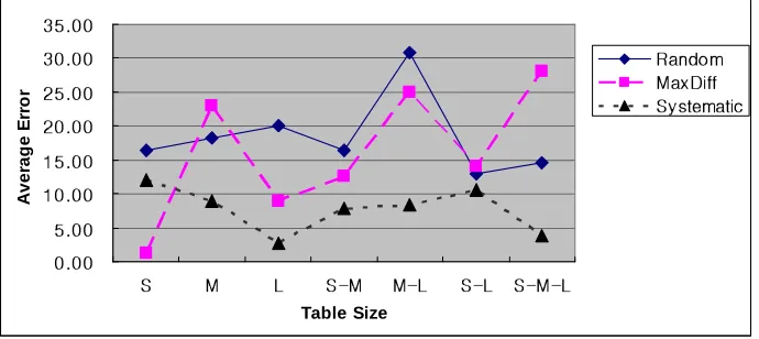
5.3.1 Effect of Table Size

Figure 5.1 shows the average relative error between actual and the result of each method as the categories of table sizes. We denote small size tables to S, medium size tables to M, large tables to L and other cases to combinations of S, M and L by experimental setup Section 5.2 in Figure 5.1. Overall, systematic sampling is better than maxdiff and simple random sampling methods. Systematic sampling method shows almost stable results for all cases except small table size. We explain more detail for the specific cases. In the case of small table sizes, maxdiff histogram method shows very accurate result that is approximately 0% relative average error. In other cases, systematic sampling is the best method. In particular, if large size of tables are used, systematic sampling has a great accuracy with a big difference to simple random sampling and maxdiff histogram. In summary, we can use maxdiff histogram when table size is greater than 0 and equal to 10,000. In other cases, it is better to use systematic sampling than other methods.

Table Size

A

v

e

ra

g

e

E

rr

o

r

(45)

5.3.2 Effect of Frequency skew

Figure 5.2 shows the average relative error as categories of the degree of skews of frequency set. We denote non skew frequency to Non, low skew to Low, medium skew to Mid and high skew to High by experimental setup Section 5.2 in this figure. Overall, results for all methods depict that the more frequencies are skewed, the more accurate the results are. MaxDiff and systematic sampling methods show similar results which have more accurate results than simple random sampling. Two methods show less than 5% average relative error. When frequencies are highly skewed, all three methods perform essentially no error (i.e.,within 3%). In summary, when data frequencies are highly skewed or not skewed, we can choose any of three methods because the average errors are almost same. On the other hand, simple random sampling is not a good method when data frequencies are low-skewed or medium-skewed. ! ! ! ! " " " " # # # # $ $ $ $ ! ! ! ! ! ! ! ! % % % % ! ! ! ! &'

()*+,- ./0(

1 -23 '44 &567 +(-7' 8

Figure 5.2: Frequency Set Estimation

(46)

Method

R

el

a

ti

v

e

E

rr

o

r

Figure 5.3: Non-Skew Data without primary key

see only values on non-primary key, systematic sampling shows the absolutely most accurate result than those of two methods with a low relative error.

5.3.3 Effect of Selectivity

Figure 5.4 demonstrates the average relative error as categories of selectivities. In the low selectivity environment, Maxdiff histogram and systematic sampling methods have relatively small errors. In contrast,high selectivity environment show opposite results. That means that simple random sampling performs slightly better than systematic sampling and maxdiff histogram. In brief, when a query has a low selectivity, it is better to choose system-atic sampling than two other methods. Otherwise, we can choose simple random sampling rather than Maxdiff histogram and systematic sampling although all three methods have low errors.

5.3.4 Effect of query conditions

(47)

!" #$%& ' ! ( %)* ++ ,-. # !% . /

Figure 5.4: Selectivity Estimation

results in range queries is that we have many candidate samples. Therefore, if many same values are in the table, they can be selected with high probabilities. Consequentially, the best method for equal query conditions is systematic sampling. We also choose all three methods for range queries and systematic sampling for join operations.

! ! ! ! " " " " # # # # $ $ $ $ % % % % " " " " & & & & # # # # # # # # ' ' ' ' # # # # ( )* ) + , -.. (/01 ) 1 2

(48)

5.3.5 Effect of Sampling Fraction

We applied 5, 10 and 15% of sampling fraction for maxdiff and systematic sampling methods. For this experiments, maxdiff histogram set the number of sample to given sampling fraction instead of using Chaudhuri’s algorithm. Maxdiff histogram in Figure 5.6 shows that we can get more accurate result when we apply 10% of sampling fraction than the case of 5%. However, we get worse result when we apply 15% of sampling fraction than the case of 10% of sampling fraction. It shows that it is not a good guideline to use too many sample values. Therefore, appropriate sampling sizes are applied rather than many sample values are used. Systematic Sampling in Figure 5.6 shows whenever we sample many values, we can get more accurate result. Therefore, the number of samples are affected on the accuracy of results.

Sample fraction

R

e

la

ti

v

e

E

r

o

r

Figure 5.6: Accuracy by Sampling Fraction

5.3.6 Elapsed Time

(49)

take much time to sample although elapsed time is exponentially growing when table size are larger. Supp lier Cus tom er Part PartS upp Ord ers Line item Table Name E la sp ed T im e (s )

Figure 5.7: Elapsed time by Table sizes

Another experiments is estimation of taken time for sample sizes. Figure 5.8 shows that simple random sampling method takes more time than other methods. When many sample values are taken in simple random sampling, it takes much time to compare and re-calculate mean and variance whenever new sample value is taken. Systematic sampling and maxdiff histogram show same patterns with the case of elapsed time for table sizes.

Sample Fraction E la sp e d T im e ( s)

(50)

5.3.7 Summary

(51)

(52)

Chapter 6

Conclusion

Decision whether materialized views will be used for a strategy for executing a query is based on the number of tuples for the query result. If a materialized view is more expensive than other available strategies, the view may not be able to be used to execute a query. When we estimate view sizes, one of the factors is a query size that consists of the view; that is the number of tuples. If the number of tuples are not correctly estimated, con-suming CPU and I/O costs may be more expensive than actual costs. Therefore, estimation of the number of tuples is a basic factor to be considered.

In this thesis, we presented three approaches for estimation of query result sizes. They are simple random sampling, maxdiff histogram and systematic sampling methods. We have used efficient methods for query size estimation in the current researches and we evaluated the accuracy of these methods in several environments. The results can be used as guidelines to choose the best method in each condition.

(53)

• Size : We can recommend MaxDiff histogram with sampling if the table sizes are small where small is between 0 and 10,000. Otherwise, systematic sampling is preferred with approximately 10% average relative error.

• Degree of skew : In this category, results show promising differences by degrees of skew. Overall, we can choose any of the three methods if the degree of skew is high or none where high is between 2 and 6 and none is between 0 and 1. In other cases of estimations, MaxDiff histogram and systematic sampling methods are preferred. • Selectivity : We can recommend systematic sampling if query selectivities are

distrib-uted between 0 and 0.2 and simple random sampling if selectivities are distribdistrib-uted between 0.8 and 1.

• Condition : We can recommend systematic sampling in all kinds of query conditions. In specific, we can select any of three methods in range queries because all methods have slight differences and there are essentially no error.

(54)

Bibliography

[1] Microsoft SQL. http://www.microsoft.com/sql/. [2] Oracle. http://www.oracle.com.

[3] PostgreSql. http://www.postgresql.org. [4] TPC-H. http://www.tpc.org.

[5] Elena Baralis, Stefano Paraboschi, and Ernest Teniente. Materialized views selection in a multidimensional database. InThe VLDB Journal, pages 156–165, 1997.

[6] Donald D. Chamberlin, Morton M. Astrahan, Michael W. Blasgen, James N. Gray, W. Frank King, Bruce G. Lindsay, Raymond Lorie, James W. Mehl, Thomas G. Price, Franco Putzolu, Patricia Griffiths Selinger, Mario Schkolnick, Donald R. Slutz, Irv-ing L. Traiger, Bradford W. Wade, and Robert A. Yost. A history and evaluation of system r. Commun. ACM, 24(10):632–646, 1981.

[7] Surajit Chaudhuri, Rajeev Motwani, and Vivek Narasayya. Random sampling for his-togram construction: how much is enough? InProceedings of the 1998 ACM SIGMOD international conference on Management of data, pages 436–447. ACM Press, 1998.

[8] Fa-Chung Fred Chen and Margaret H. Dunham. Common subexpression processing in multiple-query processing. IEEE Trans. Knowl. Data Eng., 10(3):493–499, 1998. [9] S. Christodoulakis. Implications of certain assumptions in database performance

evau-ation. ACM Trans. Database Syst., 9(2):163–186, 1984.

(55)

[11] Peter J. Haas and Arun N. Swami. Sequential sampling procedures for query size estimation. In Proceedings of the 1992 ACM SIGMOD international conference on Management of data, pages 341–350. ACM Press, 1992.

[12] Banchong Harangsri. Query Result Size Estimation Techniques in Database Systems. PhD thesis, 1998.

[13] Venky Harinarayan, Anand Rajaraman, and Jeffrey D. Ullman. Implementing data cubes efficiently. In Proceedings of the 1996 ACM SIGMOD international conference on Management of data, pages 205–216. ACM Press, 1996.

[14] Wen-Chi Hou and Gultekin Ozsoyoglu. Statistical estimators for aggregate relational algebra queries. ACM Trans. Database Syst., 16(4):600–654, 1991.

[15] Wen-Chi Hou, Gultekin Ozsoyoglu, and Baldeo K. Taneja. Processing aggregate rela-tional queries with hard time constraints. SIGMOD Rec., 18(2):68–77, 1989.

[16] Yannis E. Ioannidis. Universality of serial histograms. In Proceedings of the 19th International Conference on Very Large Data Bases, pages 256–267. Morgan Kaufmann Publishers Inc., 1993.

[17] Yannis E. Ioannidis and Viswanath Poosala. Balancing histogram optimality and prac-ticality for query result size estimation. In Proceedings of the 1995 ACM SIGMOD international conference on Management of data, pages 233–244. ACM Press, 1995.

[18] Younkyung Cha Kang. Randomized algorithms for query optimization. PhD thesis, 1991.

[19] Robert Philip Kooi. The optimization of queries in relational databases. PhD thesis, 1980.

[20] Yibei Ling and Wei Sun. An evaluation of sampling-based size estimation methods for selections in database systems. InProceedings of the Eleventh International Conference on Data Engineering, pages 532–539. IEEE Computer Society, 1995.

(56)

[22] Akifumi Makinouchi, Masayoshi Tezuka, Hajime Kitakami, and S. Adachi. The opti-mization strategy for query evaluation in rdb/v1. InVLDB, pages 518–529, 1981. [23] A. H. H. Ngu, B. Harangsri, and J. Shepherd. Query size estimation for joins using

systematic sampling. Distrib. Parallel Databases, 15(3):237–275, 2004.

[24] Gregory Piatetsky-Shapiro and Charles Connell. Accurate estimation of the number of tuples satisfying a condition. InProceedings of the 1984 ACM SIGMOD international conference on Management of data, pages 256–276. ACM Press, 1984.

[25] Viswanath Poosala, Peter J. Haas, Yannis E. Ioannidis, and Eugene J. Shekita. Im-proved histograms for selectivity estimation of range predicates. InProceedings of the ACM SIGMOD 1996 Conference, pages 294–305, 1996.

[26] P. Griffiths Selinger, M. M. Astrahan, D. D. Chamberlin, R. A. Lorie, and T. G. Price. Access path selection in a relational database management system. In Proceedings of the 1979 ACM SIGMOD international conference on Management of data, pages 23–34. ACM Press, 1979.

[27] Arun Swami and K. Bernhard Schiefer. On the estimation of join result sizes. In Proceedings of the 4th international conference on extending database technology on Advances in database technology, pages 287–300. Springer-Verlag New York, Inc., 1994.

[28] Jeffrey S. Vitter. Random sampling with a reservoir. ACM Trans. Math. Softw., 11(1):37–57, 1985.

(57)

Appendix A

A.1 TPC-H Table Layout

In this section, we explain layouts for TPC-H tables. We indicate column names, data types, sizes and primary keys.

PART Table

Column Name Data Type PARTKEY identifier

NAME variable text, size 55 MFGR fixed text, size 25 BRAND fixed text, size 10 TYPE variable text, size 25

SIZE integer

CONTAINER fixed text, size 10 RETAILPRICE decimal

COMMENT variable text, size 23 Primary Key PARTKEY

SUPPLIER Table

Column Name Data Type SUPPKEY identifier

NAME fixed text, size 25 ADDRESS variable text, size 40 NATIONKEY identifier

PHONE fixed text, size 15 ACCTBAL decimal

(58)

PARTSUPP Table

Column Name Data Type PARTKEY identifier SUPPKEY identifier AVAILQTY integer SUPPLYCOST decimal

COMMENT variable text, size 199 Primary Key PARTKEY, SUPPKEY CUSTOMER Table

Column Name Data Type CUSTKEY identifier

NAME variable text, size 25 ADDRESS variable text, size 40 NATIONKEY identifier

PHONE fixed text, size 15 ACCTBAL decimal

MKTSEGMENT fixed text, size 10 COMMENT variable text, size 117 Primary Key CUSTKEY

ORDERS Table

Column Name Data Type ORDERKEY identifier CUSTKEY identifier

ORDERSTATUS fixed text size, size 1 TOTALPRICE decimal

ORDERDATE date

ORDERPRIORITY fixed text, size 15 CLERK fixed text, size 15 SHIPPRIORITY integer

COMMENT variable text, size 79 Primary Key ORDERKEY NATION Table

Column Name Data Type NATIONKEY identifier NAME identifier REGIONKEY identifier

(59)

REGION Table

Column Name Data Type REGIONKEY identifier NAME identifier

COMMENT variable text, size 152 Primary Key REGIONKEY

LINEITEM Table

Column Name Data Type ORDERKEY identifier PARTKEY identifier SUPPKEY identifier LINENUMBER integer EXTENDEDPRICE decimal

DISCOUNT decimal

TAX decimal

RETURNFLAG fixed text, size 1 LINESTATUS fixed text, size 1

SHIPDATE date

COMMITDATE date RECEIPTDATE date

SHIPINSTRUCT fixed text, size 25 SHIPMODE fixed text, size 10 COMMENT variable text, size 44

Primary Key ORDERKEY, LINENUMBER

A.2 Queries for Experiments

In this section, we explain representative queries for each category to use experi-mental results.

A.2.1 Size Category

This category has small, medium, large, small-medium, small-large, medium-large, small-medium-large set. For each set of table sizes, we illustrate queries for experiments.

1. SMALL TABLE : Table sizes are less than or equal to 10,000. select regionkey from nation where regionkey = ’3’;

(60)

select regionkey from region where regionkey = ’4’;

select nationkey from supplier where nationkey = ’21’;

select acctbal from supplier where acctbal = 8091.65;

select suppkey from supplier where suppkey = ’3942’;

select r.regionkey, n.nationkey from nation n,region r where n.nationkey = ’17’ and r.regionkey = ’4’

and n.regioney = r.regionkey;

select * from nation n,region r where r.regionkey = n.regionkey;

select r.regionkey from nation n,region r

where n.regionkey = ’1’ and n.regionkey = r.regionkey;

select * from supplier s,nation n

where s.nationkey = ’8’ and s.nationkey = n.nationkey;

2. Medium Table : Table sizes are greater than 10,000 and less than or equal to 800,000. select custkey from customer where custkey = ’7204’;

select acctbal from customer where acctbal = 1228.24;

select mktsegment from customer where mktsegment = ’HOUSEHOLD’;

select partkey from part where partkey = ’4941’;

select mfgr from part where mfgr = ’Manufacturer#3’;

select brand from part where brand = ’Brand#43’;

select type from part where type = ’PROMO ANODIZED STEEL’;

select * from part p,partsupp ps where p.partkey = ps.partkey;

select * from part p,partsupp ps

where p.partkey = ’32’ and p.partkey = ps.partkey;

select brand from part where brand >= ’Brand#20’;

(61)

3. Large Table : Table sizes are greater than 800,000 and less than or equal to 6,001,215. select orderstatus from orders where orderstatus = ’F’;

select orderdate from orders where orderdate = date ’1992-01-23’;

select orderpriority from orders where orderpriority = ’5-LOW’;

select partkey from lineitem where partkey = ’32012’;

select linenumber from lineitem where linenumber = 4;

select orderstatus from orders o,lineitem l

where o.orderkey = l.orderkey and o.orderkey = ’1000097’;

select orderstatus from orders where orderstatus <= ’O’;

select orderdate from orders

where orderdate <= date ’1992-10-25’;

select * from lineitem where linenumber <= 5;

select * from lineitem where commitdate > date ’1992-06-21’;

4. S-M Tables : Mixed type of small and medium sizes of tables.

select * from partsupp ps,supplier s where ps.suppkey = s.suppkey;

select * from partsupp ps,supplier s

where ps.availqty >= 670 and s.suppkey = ’7310’ and ps.suppkey = s.suppkey;

select * from partsupp ps,supplier s

where ps.supplycost < 1000.00 and s.acctbal < 3000.00 and ps.suppkey = s.suppkey;

select * from customer c,supplier s where c.nationkey = s.nationkey;

select * from customer c,supplier s

(62)

select * from nation n,region r,part p

where p.retailprice >= 935.00 and r.regionkey = n.regionkey;

select * from part p,partsupp ps,customer c,nation n where p.container = ’JUMBO BOX’ and ps.supplycost = 1.00 and p.partkey = ps.partkey

and n.nationkey = c.nationkey;

select * from part p,partsupp ps,customer c,nation n where p.partkey = ps.partkey and c.acctbal <= 4000.00 and c.nationkey = n.nationkey;

select s.nationkey,p.size,ps.supplycost

from supplier s,customer c,part p,partsupp ps

where s.nationkey = ’10’ and s.nationkey = c.nationkey and p.size > 50 and ps.supplycost <= 12.00

and p.partkey = ps.partkey;

select r.name,p.size,ps.availqty

from region r,nation n,supplier s,part p,partsupp ps,customer c where r.regionkey = n.regionkey and n.regionkey = ’4’

and s.nationkey = n.nationkey

and p.size < 150 and ps.availqty >=1000 and p.partkey = ps.partkey

and c.acctbal = 6853.37

and c.nationkey = n.nationkey;

5. S-L Tables : Mixed type of small and large sizes of tables select n.name, o.orderstatus

from nation n,orders o

where n.name = ’JAPAN’ and o.orderstatus = ’F’;

select n.nationkey, o.orderpriority from nation n,orders o

where n.nationkey = ’12’ and o.orderpriority > ’3-MEDIUM’;

select clerk

from nation n,orders o

where clerk = ’Clerk#000000039’ and n.nationkey = ’22’;

select n.nationkey, l.returnflag from nation n,lineitem l

(63)

select o.orderpriority from orders o,region r

where o.orderpriority <= ’4-NOT SPECIFIED’ and r.regionkey < ’3’;

select n.nationkey, o.orderpriority from nation n,orders o,supplier s where n.nationkey = s.nationkey and o.orderpriority = ’5-LOW’;

select o.orderdate,n.nationkey from orders o,nation n,supplier s where o.orderdate >= date ’1992-09-10’ and n.nationkey = s.nationkey;

select o.clerk,n.nationkey

from orders o,nation n,supplier s where o.clerk = ’Clerk#000000028’

and n.nationkey = ’4’ and s.acctbal > 10200.00 and s.nationkey = n.nationkey;

select *

from lineitem l,nation n,region r

where l.quantity <= 1000.00 and n.regionkey = r.regionkey;

select n.regionkey, l.quantity from nation n,region r,lineitem l

where n.regionkey = r.regionkey and l.quantity > 500.00;

6. M-L Tables : Mixed type of medium and large sizes of tables. select c.custkey, c.mktsegment

from customer c,orders o where c.custkey = o.custkey;

select o.custkey, c.acctbal

from customer c,orders o where o.orderkey = ’79999’ and c.acctbal >= 8000.00 and c.custkey = o.custkey;

select c.custkey, c.mktsegment from orders o,customer c

where c.mktsegment = ’MACHINERY’ and o.clerk = ’Clerk#000000010’ and c.custkey = o.custkey;

select p.brand from part p,orders o

Query Size Estimation through Sampling

Contents

List of Figures

List of Tables

Chapter 1

Introduction

1.1

Overview of Research

1.2

Thesis Contributions

1.3

Thesis Organization

Chapter 2

Related Work

Chapter 3

Basic Concepts of Query Size

Estimation

3.1

Terminology in Database Systems

3.2

Definitions and Notations for View Size Estimation

3.3

Problem Statement

3.4

Selectivity Calculation

3.5

Query Result Size Estimation Methods

Chapter 4

Implementations

4.1

Simple Random Sampling Method

4.2

MaxDiff Histogram Method

4.3

Systematic Sampling Method

Chapter 5

Experimental Results

5.1

Notations and Definitions

5.2

Experimental Setup

5.3

Experimental Results

Chapter 6

Conclusion

Bibliography

Appendix A

A.1

TPC-H Table Layout

A.2

Queries for Experiments